July 21, 2017
BACHELOR THESIS
Regularization of 3D
dyadic Green’s function
for flat interfaces
Iris Ottens
Faculty of Science and Technology
Faculty of Electrical Engineering, Mathematics and Computer Science (EEMCS) Complex Photonics Systems (COPS)
Multiscale Modeling and Simulation(MMS)
Supervised by: Dr. S. B. Hasan
Abstract
Contents
1 Introduction 3
2 Theoretical background 4
3 Free space Green’s function 5
3.1 Eigenfunctions . . . 5
3.2 Eigenfunction expansion . . . 7
3.3 Solving the integrals . . . 8
3.4 Transverse and longitudinal parts . . . 9
3.5 Regularized problem . . . 11
4 Green’s function for a semi-infinite medium 12 5 Green’s function for a thin film 15 6 Conclusion/Outlook 25 Acknowledgements 26 References 27 A Orthogonality relations 28 B Solving parts of the integrals 28 B.1 First integral . . . 28
B.2 Second integral . . . 30
B.3 Third integral . . . 33
C Solutions of the integrals involving the regularization 34 C.1 First integral . . . 34
C.2 Second integral . . . 35
1 Introduction
Calculating the electric field produced by a current source in and around a dielectric medium, often makes use of an electric Green’s functions. The same Green’s functions can also directly be used to calculate the local density of states (LDOS) of a dipole, as the projected LDOS in a certain direction is directly dependent on the imaginary part of the Green’s function evaluated at the source [1]. This LDOS is of importance in determining the transition rates of atoms in Fermi’s Golden rule. This transition rate is
Γ = 2π
~
|hf|H0|ii|N(r), (1) where~ is Planck’s constant,f and iare the final and the initial states respectively, H0 is the dipole Hamiltonian and Np(r) is the density of states (DOS). For local variations the LDOS can be used
instead [2].
Calculating the imaginary part of the Green’s function in order to get the LDOS does not pose any problems when dealing with non absorbing media, as the imaginary part of the Green’s function at the location of the dipole is finite in that case. However, when looking at absorbing media, which all materials except for vacuum are, the dielectric constant is complex, causing the singularity in the real part of the Green’s function to also enter into the imaginary part.To solve this problem, we introduce a regularization method that basically assigns a finite size to the point dipole [3].
In this report we will specifically look at problems that have an azimuthal symmetry, such as a thin film or half plane of dielectric material. This is a relevant symmetry to, for example, light emitting diodes (LEDs) [4], which are an important application of this problem. To stay close to the solutions found in literature [5], we will approach the problem in cylindrical coordinates.
2 Theoretical background
In this section we will derive the LDOS in terms of the imaginary part of the Green’s function, corre-sponding to the electric field with a dipole as source, which sets the background of this work. We start the derivation from the macroscopic Maxwell’s equations for harmonically oscillating fields in matter with ae−iωttime dependence, whereωis the angular frequency [6].
∇ ·E(r) =ρ(r)
∇ ·H(r) = 0
∇ ×E(r) =iωµH(r)
∇ ×H(r) =J(r)−iωE(r). (2) Here E(r)andH(r)are the electric field and the magnetic field respectively, µandrespectively stand for permeability and permittivity of the considered medium,J(r)is the current density andρ(r)is
the electric charge density. From these equations and by introducingk =ω√µthe vector Helmholtz equation can be derived to be
∇ × ∇ ×E(r, ω)−k2(ω)E(r, ω) =iωµJ(r, ω). (3) The Green’s function of this equation then has to satisfy
∇ × ∇ × Ge(r,r0, ω)−k2Ge(r,r0, ω) =Iδ(r−r0), (4)
withIbeing the identity matrix andr0the location of the source [6]. For a sourceJ(r), the electric field
relates to the Green’s function by
E(r, ω) =iωµ Z Z Z
J(r, ω)· Ge(r,r0, ω)dV, (5)
with the integral going over all space [6]. For the special case of a Hertzian point dipole the source term is
J(r, ω) =−iωp(ω)δ(r−r0), (6)
withpthe dipole moment. In that case the electric field directly relates to the Green’s function as
E(r) =ω2µp(ω)· Ge(r,r0, ω). (7)
The density of states (DOS) counts the modes corresponding to a certainωwhich is expressed as
N(ω) =X
n
δ ω2−ω2n
, (8)
withωn the angular frequency corresponding to an eigenvalue of the vector Helmholtz equation. The
local density of states (LDOS) is the spatial projection of DOS given by Ne(r, ω) =
X
n
|En(r)|
2
δ ω2−ω2n
, (9)
withEn(r)a discrete set of orthonormal eigenmodes of the vector Helmholtz equation satisfying
The Green’s function can than be expressed as a superposition of these eigenmodes
Ge(r,r0, ω) =
X
n
An(r0)⊗En(r). (11)
Filling Eq. (11) in into Eq. (4) and using the orthogonality relations between the eigenmodes gives ω2n−ω2
An(r0) =c2E∗n(r0). (12)
By taking ω2n−ω2
to the other side and using the mathematical identity
lim
η→0+
1
x−iη = PV 1
x
+iπδ(x), (13)
withPVthe principle value, we get
An(r0) =c2E∗n(r0)
PV
1
ω2
n−ω2
+iπδ ω2n−ω2
. (14)
The Green’s function then becomes Ge(r,r0, ω) =
X
n
c2E∗n(r0)⊗En(r)×
PV
1
ω2
n−ω2
+iπδ ω2−ω2n
. (15)
When comparing the expression of the Green’s function with the previous expression of the LDOS, at Eq. (9), the LDOS can also be expressed as
Ne(r, ω) =
1
πc2Im [Tr{Ge(r,r, ω)}], (16)
whereImstands for the imaginary part andTrtakes the trace of the tensor. The projected LDOS, in the
direction of the dipole, can then be rewritten as
Ne,p(r, ω) =
1
πc2[p·Im{Ge(r,r, ω)} ·p]. (17)
With above it can be concluded that the imaginary part of the Green’s function at the location of the source is indeed an observable [1], namely the LDOS of a dipole, which determines the transition rate of the dipole.
3 Free space Green’s function
3.1 Eigenfunctions
We will start solving the vector Helmholtz equation for the Green’s function, Eq. (2) and (4), for free space
∇ × ∇ × Ge0(r,r0)−k2Ge0(r,r0) =Iδ(r−r0), (18)
withk=ω√µ, the same as above. In case of absorbing media the permittivity will be complex. For the sake of shortening notationGe0will be written asG0as we will only be discussing the Green’s function
for the electric field. The dependence on the spatial variables is implied, but not explicitly written in the following for the same reasons.
andL, by using the eigenfunctions of the scalar wave equation. These eigenfunctions of∇2ψ+κ2ψ= 0
can be obtained by separation of variables, which, in cylindrical coordinates, gives
ψo
e =Jn(λr) sin
cos (nφ)e
ihz, (19)
with eigenvalues
κ2=λ2+h2.
From now on the subscriptsoandethat point at the distinction between the upper and the lower part of the solution, the odd and the even parts respectively, will be omitted unless only one of these parts is considered.
With Eq. (19) we can generate the eigenfunctions of the vector Helmholtz equation mentioned above by employing the method introduced in Ref. [7] and choosing the right piloting vector. The piloting vector is used to give a direction to the eigenfunctions of Eq. (19) and can be chosen in any direction. The direction will be decided based on the geometries that are considered to make calculations easier and is thus chosen to be pointing in thezˆdirection. With this choice in pointing vector we gets the following
functions,M,NandL, that can easily be shown to be eigenfunctions of the vector Helmholtz equation
Mnλ(h) =∇ ×(ψzˆ) (20)
=∇ ×(Jn(λr)
sin cos (nφ)e
ihzzˆ)
=eihz ±rˆnJn(λr)
r
cos
sin (nφ)− ˆ
φ∂ ∂rJn(λr)
sin cos (nφ)
!
= 1
κ∇ ×Nnλ(h), (21)
Nnλ(h) =
1
κ∇ × ∇ ×(ψzˆ) (22)
= 1
κ∇ ×Mnλ(h) (23)
= 1
κe
ihz
"
ˆ
rih∂ ∂rJn(λr)
sin
cos (nφ)± ˆ
φihnJn(λr) r
cos
sin (nφ)
+ ˆz −∂
2
∂r2Jn(λr)
sin
cos (nφ) +
n2J
n(λr)
r2
sin cos (nφ)
!#
= 1
κe
ihz rihˆ ∂
∂rJn(λr)
sin
cos (nφ)± ˆ
φihnJn(λr) r
cos
sin (nφ) + ˆzλ
2J
n(λr)
sin cos (nφ)
!
and
Lnλ(h) =∇(ψ) (24)
=∇ Jn(λr)
sin cos (nφ)e
ihz
!
=eihz rˆ∂
∂rJn(λr)
sin
cos (nφ)± ˆ
φnJn(λr) r
cos
sin (nφ) + ˆzihJn(λr) sin cos (nφ)
TheM,NandLfunctions are all orthogonal to each other and to themselves ifn6=n0, proof of this can be found in Ref. [6] and in Appendix A. And with themselves they have the following normalization constants
Z Z Z
dVNnλ(h)Nnλ0(−h0) = 2π2λ(1 +δ0n)δ(h−h0)δ(λ−λ0), (25) Z Z Z
dVMnλ(h)Mnλ0(−h0) = 2π2λ(1 +δ0n)δ(h−h0)δ(λ−λ0) (26) and
Z Z Z
dVLnλ(h)Lnλ0(−h0) = 2π2(λ+ hh0
λ0 )(1 +δ0n)δ(h−h
0)δ(λ−λ0), (27)
whereδ0n denotes the Kronecker delta, being 1 ifn= 0and 0 otherwise. These constants have been
found using the method as can be found in Ref. [6].
3.2 Eigenfunction expansion
To find the solution for the Green’s function Eq. (18) will be expanded in the eigenfunctions we deter-mined in the previous section. The right side of Eq. (18), namely the delta function, can be expressed in terms of the eigenfunctions
Iδ(r−r0) =
Z ∞
−∞
dh Z ∞
0
dλ
∞
X
n=0
{Nnλ(h)anλ(h) +Mnλ(h)bnλ(h) +Lnλ(h)cnλ(h)}. (28)
Both sides of Eq. (28) will be multiplied byNnλ(−h),Mnλ(−h)andLnλ(−h)respectively and
inte-grated over space, which gives the coefficients
anλ(h) =Nnλ0(−h)/
Z ∞
−∞
dh0 Z ∞
0
dλ0 Z Z Z
dVNnλ0(h0)Nnλ(−h) (29)
=Nnλ0(−h)/(1 +δ0n)2π2λ,
bnλ(h) =Mnλ0(−h)/
Z ∞
−∞
dh0 Z ∞
0
dλ0 Z Z Z
dVMnλ0(h0)Mnλ(−h) (30)
=Mnλ0(−h)/(1 +δ0n)2π2λ
and
cnλ(h) =Lnλ0(−h)/
Z ∞
−∞
dh0 Z ∞
0
dλ0 Z Z Z
dVLnλ0(h0)Lnλ(−h) (31)
=λLnλ0(−h)/(1 +δ0n)2π2(λ2+h2).
When filling in the above mentioned coefficients into Eq. (28) we get
Iδ(r−r0) =
Z ∞
−∞
dh Z ∞
0
dλ
∞
X
n=0
1 2π2(1 +δ
0n)
{Nnλ(h)Nnλ0(−h)/λ+Mnλ(h)Mnλ0(−h)/λ+
λLnλ(h)Lnλ0(−h)/ λ2+h2 .
The Green’s function can also be expressed as a superposition of the eigenfunctions as follows
G0=
Z ∞
−∞
dh Z ∞
0
dλ
∞
X
n=0
{Nnλ(h)Anλ(h) +Mnλ(h)Bnλ(h) +Lnλ(h)Cnλ(h)}. (33)
Eq. (33), as well as the expansion of the delta function, will now be substituted back into Eq. (18) to get the coefficients. Here the relations betweenMandNare used as well as the fact that the curl ofL is zero. This leads us to
Z ∞
−∞
dh Z ∞
0
dλ
∞
X
n=0
κ2−k2Nnλ(h)Anλ(h) + κ2−k2
Mnλ(h)Bnλ(h)
−k2L
nλ(h)Cnλ(h) =
Z ∞
−∞
dh Z ∞
0
dλ
∞
X
n=0
1 2π2(1 +δ
0n)
{Nnλ(h)Nnλ0(−h)/λ+Mnλ(h)Mnλ0(−h)/λ
+λLnλ(h)Lnλ0(−h)/ (λ+h2 . (34)
By comparing the coefficients of the eigenfunctions we get
Anλ(h) =anλ(h)/ κ2−k2
=Nnλ0(−h)/ 2π2λ(1 +δ0n) κ2−k2
, (35)
Bnλ(h) =bnλ(h)/ κ2−k2
=Mnλ0(−h)/ 2π2λ(1 +δ0n) κ2−k2
(36)
and
Cnλ(h) =cnλ(h)/ −k2=−λLnλ0(−h)/ 2π2 h2+λ2(1 +δ0n)k2. (37)
Filling in the coefficients found above gives a solution of the Green’s function in terms of the eigen-functions
G0=
Z ∞
−∞
dh Z ∞
0
dλ
∞
X
n=0
N
nλ(h)Nnλ0(−h)
(1 +δ0n) 2π2λ(κ2−k2)
+ Mnλ(h)Mnλ0(−h) (1 +δ0n) 2π2λ(κ2−k2)
+ −λLnλ(h)Lnλ0(−h) (1 +δ0n) 2π2(h2+λ2)k2
. (38)
3.3 Solving the integrals
We now have the Green’s function in terms of the eigenfunctions of the vector Helmholtz equation. This solution, however, still contains some integrals. Of these the integral with respect tohnecessary to solve for the application of the boundary conditions. This will be done by making use of contour integration in the complex plane. The function only has simple poles, which makes it easy to use the residue theorem. The details can be found in Appendix B.
G0=
Z ∞
0
dλ
∞
X
n=0
i
2 (1 +δ0n)πλ
√ k2−λ2
h Nnλ
p
k2−λ2N
nλ0
−pk2−λ2
+Mnλ
p
k2−λ2M
nλ0
−pk2−λ2i
− λ k2(1 +δ
0n)π
Jn(λr)Jn(λr0)
sin cos (nφ)
sin
cos (nφ0)δ(z−z0)ˆzzˆ0
) (39)
and forz < z0
G0=
Z ∞
0
dλ
∞
X
n=0
i
2 (1 +δ0n)πλ
√ k2−λ2
h Nnλ
−pk2−λ2N
nλ0
p
k2−λ2
+Mnλ
−pk2−λ2M
nλ0
p
k2−λ2i.
− λ k2(1 +δ
0n)π
Jn(λr)Jn(λr0)
sin
cos (nφ) sin
cos (nφ0)δ(z−z0)ˆzzˆ0
) (40)
We will not analytically solve the integral with respect toλ. When trying a similar approach as with the one for h, three problems can be found. Firstly, the integral goes from zero to infinity instead of from - to + infinity. This can be solved as seen in Ref. [6]. Additionally there is also the problem of the pole atλ= 0lying on the contour if the same contour is used as forh. This is also easily to solved by going around it, thus having a contribution of πiinstead of 2πi. The last problem is the square root, which is multi valued. For this a branch cut must be created between the branch points, which the contour is not allowed to cross. This might be done in a way similar to what was done in ref. [8]. However the contour integral still remains too challenging for analytical calculations. Therefore, the standard practice of numerically integrating Eqs.(??-??) is recommended. As this is not the main problem of what we want to solve in this report, the numerical solution will be considered at a later time.
3.4 Transverse and longitudinal parts
As the strength of singularity of the Green’s function at the location of the origin is different for the transverse and longitudinal parts of the Green’s function [3], thus we will separately look at these parts, GT
0 and G0L respectively [3]. It is easy to see that the M and N eigenfunctions correspond to the
transverse part and the L eigenfunctions to the longitudinal part, as it follows from the definition of these functions that the divergence of the first two is zero while the curl of the last one equals zero. This gives before the integration
GT
0 =
Z ∞
−∞
dh Z ∞
0
dλ
∞
X
n=0
N
nλ(h)Nnλ0(−h)
(1 +δ0n)2π2λ(κ2−k2)
+ Mnλ(h)Mnλ0(−h) (1 +δ0n)2π2λ(κ2−k2)
(41)
and
GL
0 =
Z ∞
−∞
dh Z ∞
0
dλ
∞
X
n=0
−λLnλ(h)Lnλ0(−h)
(1 +δ0n)2π2(h2+λ2)k2
. (42)
GT 0 = Z ∞ 0 dλ ∞ X n=0 ( iNnλ √
k2−λ2
Nnλ0 −
√
k2−λ2
+iMnλ
√
k2−λ2
Mnλ0 −
√
k2−λ2
2 (1 +δ0n)πλ
√ k2−λ2
+GA+ (43) and GL 0 = Z ∞ 0 dλ ∞ X n=0 (
−Lnλ(iλ)Lnλ0(−iλ)
2(1 +δ0n)πk2
− λ k2(1 +δ
0n)π
Jn(λr)Jn(λr0)
sin
cos (nφ) sin
cos (nφ0)δ(z−z0)ˆzzˆ0
) ,
(44) with
GA+=exp[−λ(z−z0)] 2k2(1 +δ
0n)π
∂
∂rJn(λr) ∂ ∂r0
Jn(λr0)
sin
cos (nφ) sin
cos (nφ0) ˆrrˆ0
+n
2
rr0
Jn(λr)Jn(λr0)
cos
sin (nφ) cos
sin (nφ0) ˆφ ˆ
φ0 ±
∂ ∂rJn(λr)
n r0
Jn(λr0)
sin
cos (nφ) cos
sin (nφ0) ˆr ˆ
φ0
± ∂ ∂r0
Jn(λr0)
n rJn(λr)
sin
cos (nφ0) cos
sin (nφ) ˆr0 ˆ
φ−λ2Jn(λr)Jn(λr0)
sin
cos (nφ) sin
cos (nφ0) ˆzzˆ0
+λ ∂
∂rJn(λr)Jn(λr0)
sin
cos (nφ) sin
cos (nφ0) ˆrˆz0−λ
∂ ∂r0
Jn(λr0)Jn(λr)
sin
cos (nφ0) sin
cos (nφ) ˆr0zˆ
±iλn
rJn(λr)Jn(λr0)
cos
sin (nφ) sin
cos (nφ0) ˆφzˆ0∓λ
n r0
Jn(λr)Jn(λr0)
cos
sin (nφ0) sin
cos (nφ) ˆφ0zˆ
! . (45)
Similarly, forz < z0
GT 0 = Z ∞ 0 dλ ∞ X n=0 (
iNnλ −
√
k2−λ2 Nnλ0
√
k2−λ2
+iMnλ −
√
k2−λ2 Mnλ0
√
k2−λ2
2 (1 +δ0n)πλ
√ k2−λ2
+GA− (46) and GL 0 = Z ∞ 0 dλ ∞ X n=0 (
−Lnλ(−iλ)Lnλ0(iλ))
2(1 +δ0n)πk2
− λ k2(1 +δ
0n)π
Jn(λr)Jn(λr0)
sin cos (nφ)
sin
cos (nφ0)δ(z−z0)ˆzzˆ0
) ,
GA−= exp[λ(z−z0)] 2k2(1 +δ
0n)π
∂ ∂rJn(λr)
∂ ∂r0
Jn(λr0)
sin
cos (nφ) sin
cos (nφ0) ˆrˆr0
+n
2
rr0
Jn(λr)Jn(λr0)
cos
sin (nφ) cos
sin (nφ0) ˆφ ˆ
φ0 ±
∂ ∂rJn(λr)
n r0
Jn(λr0)
sin
cos (nφ) cos
sin (nφ0) ˆr ˆ
φ0
± ∂ ∂r0
Jn(λr0)
n rJn(λr)
sin
cos (nφ0) cos
sin (nφ) ˆr0 ˆ
φ−λ2Jn(λr)Jn(λr0)
sin
cos (nφ) sin
cos (nφ0) ˆzzˆ0
−λ ∂
∂rJn(λr)Jn(λr0)
sin
cos (nφ) sin
cos (nφ0) ˆrˆz0+λ
∂ ∂r0
Jn(λr0)Jn(λr)
sin
cos (nφ0) sin
cos (nφ) ˆr0zˆ
∓iλn
rJn(λr)Jn(λr0)
cos
sin (nφ) sin
cos (nφ0) ˆφzˆ0±λ
n r0
Jn(λr)Jn(λr0)
cos
sin (nφ0) sin
cos (nφ) ˆφ0zˆ
! . (48)
Now that the longitudinal and traverse parts of the Green’s function have been identified, we can start the regularization process.
3.5 Regularized problem
The Green’s function derived in the previous section contains singularities, in which the one of the longitudinal part is the strongest. To solve the problem of this singularity, both parts of the Green’s function need to be regularized. This will be done by introducing two low pass filters, by the method introduced in Ref. [3]. Here the physical meaning of these filters have already been described, with the parameter 1
ΛL being proportional to the size of the source. There the filters are used in momentum
space, which corresponds to theκdomain in our solutions. The singularities are connected to largeκ values, which are made to die out by the filters. In physical therms, this grants a finite size to the source, which was originally regarded as a point source, as mentioned above in the meaning of the parameter. The actual filters for the transverse and longitudinal parts respectively are
fT(ΛT, κ) =
Λ2
T
Λ2
T+κ2
(49) and
fL(ΛL, κ) =
Λ4
L
Λ4L+κ4. (50)
As the non integrable singularity of the longitudinal part is stronger than the one in the transverse part, which is integrable, the low pass filter that is used has to be stronger as well. Adding these to the Green’s function before the integration tohwas done, Eqs. (39) and (40) gives the following regularized Green’s functions
˜
G0T =
Z ∞
−∞
dh Z ∞
0
dλ
∞
X
n=0
Λ2
T
Λ2
T +κ2
N
nλ(h)Nnλ0(−h)
(1 +δ0n)2π2λ(κ2−k2)
+ Mnλ(h)Mnλ0(−h) (1 +δ0n)2π2λ(κ2−k2)
(51)
for the transverse part and
˜
G0L=
Z ∞
−∞
dh Z ∞
0
dλ
∞
X
n=0
Λ4
L
Λ4
L+κ4
−λLnλ(h)Lnλ0(−h)
(1 +δ0n)2π2(h2+λ2)k2 (52)
The filter adds an additional simple poles at respectivelyh=±ip
Λ2
T +λ2andh=±
p ±iΛ2
L−λ2
to the previously calculated integrals. By taking these into account when using the residue theorem, as can be found in Appendix C the following expressions are found. Forz > z0
˜ GT 0 = Z ∞ 0 dλ ∞ X n=0 Λ2 T
2(1 +δ0n)πλ(k2+ Λ2T)
( i Mnλ
√
k2−λ2
Mnλ0 −
√
k2−λ2
+Nnλ
√
k2−λ2
Nnλ0 −
√
k2−λ2 √
k2−λ2 −
Mnλ
ipΛ2
T+λ2
Mnλ0
−ip
Λ2
T +λ2
+Nnλ
ipΛ2
T +λ2
Nnλ0
−ip
Λ2
T+λ2
p
Λ2
T+λ2
+ Λ
2
T
Λ2
T +k2
GA+ (53) and ˜ GL 0 = Z ∞ 0 dλ ∞ X n=0 (
−Lnλ(iλ)Lnλ0(−iλ)
2(1 +δ0n)πk2
+λiLnλ(
p iΛ2
L−λ2)Lnλ0(−
p iΛ2
L−λ2)
4(1 +δ0n)πk2
p iΛ2
L−λ2
+
λiLnλ(
p −iΛ2
L−λ2)Lnλ0(−
p −iΛ2
L−λ2)
4(1 +δ0n)πk2
p −iΛ2
L−λ2
) . (54) Likewise forz < z0
˜ GT 0 = Z ∞ 0 dλ ∞ X n=0
Λ2T
2(1 +δ0n)πλ(k2+ Λ2T)
(
i Mnλ −
√
k2−λ2 Mnλ0
√
k2−λ2
+Nnλ −
√
k2−λ2 Nnλ0
√
k2−λ2 √
k2−λ2 −
Mnλ
−ip
Λ2
T +λ2
Mnλ0
ipΛ2
T +λ2
+Nnλ
−ip
Λ2
T+λ2
Nnλ0
ipΛ2
T+λ2
p
Λ2
T+λ2
+ Λ
2
T
Λ2
T +k2
GA− (55) and ˜ GL 0 = Z ∞ 0 dλ ∞ X n=0 (
−Lnλ(−iλ)Lnλ0(iλ)
2(1 +δ0n)πk2
+λiLnλ(−
p iΛ2
L−λ2)Lnλ0(
p iΛ2
L−λ2)
4(1 +δ0n)πk2
p iΛ2
L−λ2
+
λiLnλ(−
p −iΛ2
L−λ2)Lnλ0(
p −iΛ2
L−λ2)
4(1 +δ0n)πk2
p −iΛ2
L−λ2
) . (56) This concludes the regularization of the free space Green’s function. In the next chapters some impor-tant geometries will be treated.
4 Green’s function for a semi-infinite medium
Gs. The full Green’s function is then
Ge=G0+Gs (57)
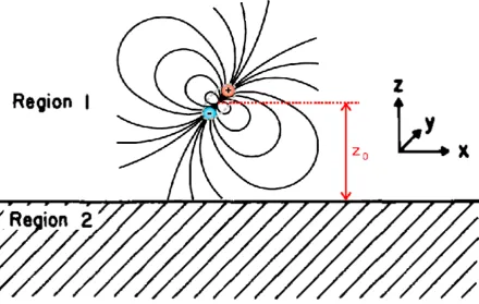
In this section the scattering part,Gs, will be calculated for the semi-infinite medium. The medium will
[image:14.595.81.522.171.450.2]divide the space into two regions, the first above the medium and the second within it. This can be seen in Fig. (1). These will be respectively called regions 1 and 2, the scattered part of the Green’s
Figure 1:A semi-infinite medium up toz= 0with a dipole above it. The figure is adapted from Ref. [4]
and [9].
function is now denoted asGs(ij), in whichi, j∈ {1,2}, denoting the region in which the Green’s function
is evaluated and region in which the dipole is positioned respectively. The boundary between the two regions is atz= 0without loss of generality. This gives the following functions for a dipole placed above
the slab, in whichhi =
p k2
i −λ2for compactness of notation, the free space Green’s function is also
given in this new notation for0< z < z0, withz0the position of the dipole along thez-axis,
G0=
Z ∞
0
dλ
∞
X
n=0
i
2 (1 +δ0n)πλh1
{Mnλ(−h1)Mnλ0(h1) +Nnλ(−h1)Nnλ0(h1)}. (58)
The scattering part above the interface, where the dipole is located is
G(11)
s =
Z ∞
0
dλ
∞
X
n=0
i
2 (1 +δ0n)πλh1
{aMnλ(h1)Mnλ0(h1) +cNnλ(h1)Nnλ0(h1)} (59)
and below the interface
G(21)
s =
Z ∞
0
dλ
∞
X
n=0
i
2 (1 +δ0n)πλh1
The termsMnλ0(h1)andNnλ0(h1)are chosen instead ofMnλ0(−h1)andNnλ0(−h1)in order to
match the free space Green’s function at the boundary. The choice betweenMnλ(h1)andMnλ(−h1)
is made with the concern of wanting the functions to die out when going to z = ∞ and z = −∞ respectively, as required by the radiation boundary condition. This is similar to the methods used in Ref. [5] and [6]. The coefficientsa, b, c and dare the scattering coefficients that will be determined below.
The scattering coefficients will be found by looking at the boundary conditions for the electric and magnetic fields. The tangential electric field, and thus the tangential component of the Green’s function, has to be continues at the boundary. The same goes for the magnetic field, which is proportional to the curl of the electric field, as long as there is no current present across the boundary. Thus employing the boundary conditions, first for the electric field, which is
ˆ
z×hG0+Gs(11)
i
= ˆz× G(21)
s . (61)
By expanding all the terms, the above mentioned equation translates to
Z ∞
0
dλ
∞
X
n=0
i
2 (1 +δ0n)πλh1
ˆ
z×[{Mnλ(−h1) +aMnλ(h1)}Mnλ0(h1)
+{Nnλ(−h1) +cNnλ(h1)}Nnλ0(h1)] =
Z ∞
0
dλ
∞
X
n=0
i
2 (1 +δ0n)πλh1
ˆ
z×[bMnλ(−h2)Mnλ0(h1)
+dNnλ(−h2)Nnλ0(h1)]. (62)
If we then compare the coefficients forMnλ0(h1)andNnλ0(h1)we get
1 +a=b (63)
and
h1
k1
(−1 +c) =−h2 k2
d. (64)
Two more equations are necessary to uniquely determine the coefficients. For this we use the continuity of the tangential magnetic field at the interfaces
1
µ1
ˆ
z× ∇ ×hG0+Gs(11)
i
= 1
µ2
ˆ
z× ∇ × G(21)
s . (65)
When expanding all the terms in Eq. (65) we get
1
µ1
Z ∞
0
dλ
∞
X
n=0
i
2 (1 +δ0n)πλh1
ˆ
z× ∇ ×[{Mnλ(−h1) +aMnλ(h1)}Mnλ0(h1)
+{Nnλ(−h1) +cNnλ(h1)}Nnλ0(h1)] =
1
µ2
Z ∞
0
dλ
∞
X
n=0
i
2 (1 +δ0n)πλh1
ˆ
z× ∇ ×[bMnλ(−h2)Mnλ0(h1)
+dNnλ(−h2)Nnλ0(h1)]. (66)
k1
µ1
Z ∞
0
dλ
∞
X
n=0
i
2 (1 +δ0n)πλh1
ˆ
z×[{Nnλ(−h1) +aNnλ(h1)}Mnλ0(h1)
+{Mnλ(−h1) +cMnλ(h1)}Nnλ0(h1)] =
k2
µ2
Z ∞
0
dλ
∞
X
n=0
i
2 (1 +δ0n)πλh1
ˆ
z×[bNnλ(−h2)Mnλ0(h1)
+dMnλ(−h2)Nnλ0(h1)]. (67)
From once again comparing the coefficients forMnλ0(h1)andNnλ0(h1)we get
h1
µ1
(−1 +a) =−h2 µ2
b (68)
and
k1
µ1
(1 +c) = k2
µ2
d. (69)
The above mentioned equations then give the following answer, Eq. (70), for the scattering coeffi-cients, thus completing the solution.
a= h1µ2−h2µ1
h1µ2−h2µ1
b= 2h1µ2
h1µ2−h2µ1
c=k22h1µ1+(1−2µ1)k21h2µ2
k2
2h1µ1+k21h2µ2
d= 2µ1µ2k1k2h1
k2
2h1µ1+k12h2µ2
(70)
Unlike with the free space Green’s function, the scattering part does not need to be regularized. Since the distance from the source to the interface is chosen much larger than the size of the source. This choice is made to prevent distortion to the current distribution of the regularized dipole that was found for free-space, which would bring difficulties beyond the scope of this report. Thus the source will be far away from the surface compared to its size, allowing the dipole to still be approximated as a point dipole with regard to scattering, thus the scattering part of the Green’s function does not need to be regularized.
5 Green’s function for a thin film
Another important geometry to look at, is that of a thin film. As discussed before, this is an important geometry when discussing problems concerning LEDs [4]. The Green’s function in the source medium can for this problem once again be divided in a part for free space and a scattering part. In this chapter the scattering part for a thin film will be calculated in a similar way to the previous section. We will look at a thin film that is infinite in theˆrdirection. This will divide the space into three regions, the ones above, in and below the thin film, as can be seen in Fig. (2). These will be respectively called regions 1, 2 and 3. The scattered part of the Green’s function will now be denoted asG(sij), in whichi, j∈ {1,2,3}. Here
the first number indicates the region in which the Green’s function is evaluated and the second indicates the region in which the dipole is located. This gives the following expressions in whichhi =
p k2
i −λ2
Figure 2:A film, of thickness d, dividing the space into three regions with a dipole inside the film, the figure is adapted from Ref. [4] and [9].
is the dipole being positioned in either region 1, 2 or 3, in which the second is the most important when considering LEDs.
For the dipole in region 1 we get
G(11)
s =
Z ∞
0
dλ
∞
X
n=0
i
2 (1 +δ0n)πλh1
{a1Mnλ(h1)Mnλ0(h1) +c1Nnλ(h1)Nnλ0(h1)}, (71)
G(31)
s =
Z ∞
0
dλ
∞
X
n=0
i
2 (1 +δ0n)πλh1
{b3Mnλ(−h3)Mnλ0(h1) +d3Nnλ(−h3)Nnλ0(h1)}, (72)
G(21)
s =
Z ∞
0
dλ
∞
X
n=0
i
2 (1 +δ0n)πλh1
{a2Mnλ(h2)Mnλ0(h1) +c2Nnλ(h2)Nnλ0(h1) +
For this case once more the free space Green’s function for z1 < z < z0, withz1 the position of the
boundary between region 1 and 2 is expressed as
G0=
Z ∞
0
dλ
∞
X
n=0
i
2 (1 +δ0n)πλh1
{Mnλ(−h1)Mnλ0(h1) +Nnλ(−h1)Nnλ0(h1)}. (74)
Secondly, for the case of the dipole being located in region 2 we have
Gs(12)=
Z ∞
0
dλ
∞
X
n=0
i
2 (1 +δ0n)πλh2
Mnλ(h1)
a+1Mnλ0(h2) +a−1Mnλ0(−h2)
+Nnλ(h1)
c+1Nnλ0(h2) +c−1Nnλ0(−h2) , (75)
G(32)
s =
Z ∞
0
dλ
∞
X
n=0
i
2 (1 +δ0n)πλh2
Mnλ(−h3)b+3Mnλ0(h2) +b−3Mnλ0(−h2)
+Nnλ(−h3)d+3Nnλ0(h2) +d−3Nnλ0(−h2) , (76)
G(22)
s =
Z ∞
0
dλ
∞
X
n=0
i
2 (1 +δ0n)πλh2
Mnλ(h2)
a+2Mnλ0(h2) +a−2Mnλ0(−h2)
+Nnλ(h2)
c+2Nnλ0(h2) +c−2Nnλ0(−h2) +Mnλ(−h2)
b+2Mnλ0(h2) +b−2Mnλ0(−h2)
+Nnλ(−h2)
d+2Nnλ0(h2) +d−2Nnλ0(−h2) . (77)
The free space Green’s function forz0< z < z1is
G0=
Z ∞
0
dλ
∞
X
n=0
i
2 (1 +δ0n)πλh1
(Mnλ(h2)Mnλ0(−h2) +Nnλ(h2)Nnλ0(−h2)) (78)
and forz3< z < z0, wherez3is the position of the boundary between region 2 and 3, Fig. (2),
G0=
Z ∞
0
dλ
∞
X
n=0
i
2 (1 +δ0n)πλh1
(Mnλ(−h2)Mnλ0(h2) +Nnλ(−h2)Nnλ0(h2)). (79)
Lastly for the dipole being positioned in region 3 we write
Gs(13)=
Z ∞
0
dλ
∞
X
n=0
i
2 (1 +δ0n)πλh3
{a1Mnλ(h1)Mnλ0(−h3) +c1Nnλ(h1)Nnλ0(−h3)}, (80)
G(33)
s =
Z ∞
0
dλ
∞
X
n=0
i
2 (1 +δ0n)πλh3
{b3Mnλ(−h3)Mnλ0(−h3) +d3Nnλ(−h3)Nnλ0(−h3)}, (81)
G(23)
s =
Z ∞
0
dλ
∞
X
n=0
i
2 (1 +δ0n)πλh3
{a2Mnλ(h2)Mnλ0(−h3) +c2Nnλ(h2)Nnλ0(−h3) +
and the free space Green’s function forz0< z < z3
G0=
Z ∞
0
dλ
∞
X
n=0
i
2 (1 +δ0n)πλh1
{Mnλ(h3)Mnλ0(−h3) +Nnλ(h3)Nnλ0(−h3)}. (83)
To determine the coefficients we will first look at the situation where the dipole is located in the first region. To get the coefficients, we’ll employ the boundary conditions on the boundary between region 1 and 2 and between 2 and 3, the same as which has been done with the slab. Firstly at the 1-2 boundary, z=z1
ˆ
z×hG0+Gs(11)
i
= ˆz× G(21)
s . (84)
Substituting the fields into the expression gives
Z ∞
0
dλ
∞
X
n=0
i
2 (1 +δ0n)πλh1
ˆ
z×[{Mnλ(−h1) +a1Mnλ(h1)}Mnλ0(h1)
+{Nnλ(−h1) +c1Nnλ(h1)}Nnλ0(h1)] =
Z ∞
0
dλ
∞
X
n=0
i
2 (1 +δ0n)πλh1
ˆ
z×[{a2Mnλ(h2) +b2Mnλ(−h2)}Mnλ0(h1)
+{c2Nnλ(h2) +d2Nnλ(−h2)}Nnλ0(h1)]. (85)
If we then compare the coefficients forMnλ0(h1)andNnλ0(h1)we get
e−ih1z1+a
1eih1z1 =a2eih2z1+b2e−ih2z1 (86)
and
h1
k1
−e−ih1z1+c
1eih1z1
=h2
k2
c2eih2z1−d2e−ih2z1
. (87)
Likewise at the 2-3 boundary,z=z3
ˆ
z× G(21)
s = ˆz× G
(31)
s . (88)
Substituting the fields into the expression gives
Z ∞
0
dλ
∞
X
n=0
i
2 (1 +δ0n)πλh1
ˆ
z×[{a2Mnλ(h2) +b2Mnλ(−h2)}Mnλ0(h1)
+{c2Nnλ(h2) +d2Nnλ(−h2)}Nnλ0(h1)] =
Z ∞
0
dλ
∞
X
n=0
i
2 (1 +δ0n)πλh1
ˆ
z×[b3Mnλ(−h3)Mnλ0(h1) +d3Nnλ(−h3)Nnλ0(h1)]. (89)
Once again we compare the coefficients forMnλ0(h1)andNnλ0(h1)we get
a2eih2z3+b2e−ih2z3=b3e−ih3z3 (90)
and
h2
k2
c2eih2z3−d2e−ih2z3=−
h3
k3
Four more equations are necessary to uniquely determine the coefficients. To get these equations we use the continuity of the tangential magnetic field at the interfaces. Once again firstly for the interface between medium 1 and 2
1
µ1
ˆ
z× ∇ ×hG0+Gs(11)
i
= 1
µ2
ˆ
z× ∇ × G(21)
s , (92)
which translates to
1
µ1
Z ∞
0
dλ
∞
X
n=0
i
2 (1 +δ0n)πλh1
ˆ
z× ∇ ×[{Mnλ(−h1) +a1Mnλ(h1)}Mnλ0(h1)
+{Nnλ(−h1) +c1Nnλ(h1)}Nnλ0(h1)] =
1
µ2
Z ∞
0
dλ
∞
X
n=0
i
2 (1 +δ0n)πλh1
ˆ
z× ∇ ×[{a2Mnλ(h2) +b2Mnλ(−h2)}Mnλ0(h1)
+{c2Nnλ(h2) +d2Nnλ(−h2)}Nnλ0(h1)]. (93)
We can then use the relations [Eqs. (21-23)] betweenMandNto get
k1
µ1
Z ∞
0
dλ
∞
X
n=0
i
2 (1 +δ0n)πλh1
ˆ
z×[{Nnλ(−h1) +a1Nnλ(h1)}Mnλ0(h1)
+{Mnλ(−h1) +c1Mnλ(h1)}Nnλ0(h1)] =
k2
µ2
Z ∞
0
dλ
∞
X
n=0
i
2 (1 +δ0n)πλh1
ˆ
z×[{a2Nnλ(h2) +b2Nnλ(−h2)}Mnλ0(h1)
+{c2Mnλ(h2) +d2Mnλ(−h2)}Nnλ0(h1)]. (94)
Once again from comparing the coefficients forMnλ0(h1)andNnλ0(h1)we get
h1
µ1
−e−ih1z1+a
1eih1z1
= h2
µ2
a2eih2z1−b2e−ih2z1
(95) and
k1
µ1
e−ih1z1+c
1eih1z1=
k2
µ2
c2eih2z1+d2e−ih2z1. (96)
Similarly, at the interface between medium 2 and 3 we have
1
µ2
ˆ
z× ∇ × G(21)
s =
1
µ3
ˆ
z× ∇ × G(31)
s (97)
which gives
1
µ2
Z ∞
0
dλ
∞
X
n=0
i
2 (1 +δ0n)πλh1
ˆ
z× ∇ ×[{a2Mnλ(h2) +b2Mnλ(−h2)}Mnλ0(h1)
+{c2Nnλ(h2) +d2Nnλ(−h2)}Nnλ0(h1)] =
1
µ3
Z ∞
0
dλ
∞
X
n=0
i
2 (1 +δ0n)πλh1
ˆ
z× ∇ ×[b3Mnλ(−h3)Mnλ0(h1) +d3Nnλ(−h3)Nnλ0(h1)]. (98)
k2 µ2 Z ∞ 0 dλ ∞ X n=0 i
2 (1 +δ0n)πλh1
ˆ
z× ∇ ×[{a2Nnλ(h2) +b2Nnλ(−h2)}Mnλ0(h1)
+{c2Mnλ(h2) +d2Mnλ(−h2)}Nnλ0(h1)] =
k3 µ3 Z ∞ 0 dλ ∞ X n=0 i
2 (1 +δ0n)πλh1
ˆ
z× ∇ ×[b3Nnλ(−h3)Mnλ0(h1) +d3Mnλ(−h3)Nnλ0(h1)]. (99)
When once again comparing the coefficients forMnλ0(h1)andNnλ0(h1)we get
h2
µ2
a2eih2z3−b2e−ih2z3=
h3
µ3
−b3e−ih3z3 (100)
and
k2
µ2
c2eih2z3+d2e−ih2z3
= k3
µ3
d3e−ih3z3
. (101)
To get the coefficients we now only need to solve the following set of equations
a1eih1z1−a2eih2z1−b2e−ih2z1 =−e−ih1z1 [1]
h1
k1c1e
ih1z1−h2
k2 c2e
ih2z1−d
2e−ih2z1
= h1
k1e
−ih1z1 [2]
a2eih2z3+b2e−ih2z3−b3e−ih3z3 = 0 [3]
h2
k2 c2e
ih2z3−d
2e−ih2z3
+h3
k3d3e
−ih3z3 = 0 [4]
h1
µ1a1e
ih1z1−h2
µ2 a2e
ih2z1−b
2e−ih2z1
=h1
µ1e
−ih1z1 [5]
k1
µ1c1e
ih1z1−k2
µ2 c2e
ih2z1+d
2e−ih2z1=−µk1
1e
−ih1z1 [6]
h2
µ2 a2e
ih2z3−b
2e−ih2z3+hµ3
3b3e
−ih3z3= 0 [7]
k2
µ2 c2e
ih2z3+d
2e−ih2z3
−k3
µ3 d3e
−ih3z3= 0 [8]
(102)
In case of the dipole being in the third region, the calculations are symmetric to those of the dipole being in the first region. This gives the following system of equations:
b3e−ih3z3−a2eih2z3−b2e−ih2z3 =−eih3z3 [1]
−h3
k3d3e
−ih3z3−h2
k2 c2e
ih2z3−d
2e−ih2z3
=−h3
k3e
ih3z3 [2]
a2eih2z1+b2e−ih2z1−a1eih1z1 = 0 [3]
h2
k2 c2e
ih2z1−d
2e−ih2z1
−h1
k1c1e
ih1z1= 0 [4]
−h3
µ3b3e
−ih3z3−h2
µ2 a2e
ih2z3−b
2e−ih2z3
=−h3
µ3e
ih3z3 [5]
k3
µ3d3e
−ih3z3−k2
µ2 c2e
ih2z3+d
2e−ih2z3=µk3
3e
−ih3z3 [6]
h2
µ2 a2e
ih2z1−b
2e−ih2z1−hµ1
1 a1e
ih1z1= 0 [7]
k2
µ2 c2e
ih2z1+d
2e−ih2z1
−k1
µ1 c1e
ih1z1= 0 [8]
(103)
Lastly we will consider the case of the dipole being in the second region. The coefficients for this case will be calculated by the same method as before by applying the boundary conditions and the continuity of the tangential magnetic field at the interfaces. Firstly, the boundary condition at the 1-2 boundary,z=z1is
ˆ
z×hG0+Gs(22)
i
Substituting the fields from Eqs. (75), (77) and (78) into the expression gives
Z ∞
0
dλ
∞
X
n=0
i
2 (1 +δ0n)πλh2
ˆ
z×
Mnλ(h2) +a−2Mnλ(h2) +b−2Mnλ(−h2) Mnλ0(−h2)
+
a+2Mnλ(h2) +b+2Mnλ(−h2) Mnλ0(h2) +
Nnλ(h2) +c−2Nnλ(h2) +d−2Nnλ(−h2) Nnλ0(−h2) +
c+2Nnλ(h2) +d+2Nnλ(−h2) Nnλ0(h2)
=
Z ∞
0
dλ
∞
X
n=0
i
2 (1 +δ0n)πλh2
ˆ
z×
Mnλ(h1)
a+1Mnλ0(h2) +a−1Mnλ0(−h2)
+Nnλ(h1)
c+1Nnλ0(h2) +c−1Nnλ0(−h2) . (105)
If we then compare the coefficients forMnλ0(h1),Nnλ0(h1),Mnλ0(−h1)andNnλ0(−h1)we get
a+2eih2z1+b+
2e
−ih2z1 =a+
1e
ih1z1, (106)
h2
k2
c+2eih2z1−d+
2e
−ih2z1= h1
k1
c+1eih1z1, (107)
eih2z1+a−
2e
ih2z1+b−
2e−
ih2z1 =a−
1e
ih1z1 (108)
and
h2
k2
eih2z1+c−
2e
ih2z1−d−
2e
−ih2z1= h1
k1
c−1eih1z1. (109)
And at the 2-3 boundary,z=z3,
ˆ
z×hG0+Gs(22)
i
= ˆz× G(32)
s . (110)
Substituting the fields from Eqs. (76), (77) and (79) into the expression gives
Z ∞
0
dλ
∞
X
n=0
i
2 (1 +δ0n)πλh2
ˆ
z×
a−2Mnλ(h2) +b−2Mnλ(−h2) Mnλ0(−h2)
+
Mnλ(−h2) +a+2Mnλ(h2) +b+2Mnλ(−h2) Mnλ0(h2) +
c−2Nnλ(h2) +d−2Nnλ(−h2) Nnλ0(−h2) +
Nnλ(−h2) +c+2Nnλ(h2) +d+2Nnλ(−h2) Nnλ0(h2)
=
Z ∞
0
dλ
∞
X
n=0
i
2 (1 +δ0n)πλh2
ˆ
z×
Mnλ(−h3)
b+3Mnλ0(h2) +b−3Mnλ0(−h2)
+Nnλ(−h3)
d+3Nnλ0(h2) +d−3Nnλ0(−h2) . (111)
Once again we compare the coefficients forMnλ0(h1),Nnλ0(h1),Mnλ0(−h1)andNnλ0(−h1)we
get
e−ih2z3+a+
2e
ih2z3+b+
2e
−ih2z3 =b+
3e
−ih3z3, (112)
h2
k2
−e−ih2z3+c+
2e
ih2z3−d+
2e
−ih2z3=h3
k3
−d+ 3e
−ih3z3, (113)
and
h2
k2
c−2eih2z3−d−
2e
−ih2z3= h3
k3
−d−3e−ih3z3. (115)
Next we’ll consider the continuity of the tangential magnetic field at the interfaces. Once again firstly for the interface between 1 and 2
1
µ2
ˆ
z× ∇ ×hG0+Gs(22)
i
= 1
µ1
ˆ
z× ∇ × G(12)
s . (116)
Which translates to
1
µ1
Z ∞
0
dλ
∞
X
n=0
i
2 (1 +δ0n)πλh2
ˆ
z× ∇ ×
Mnλ(h2) +a−2Mnλ(h2) +b−2Mnλ(−h2) Mnλ0(−h2)
+
a+2Mnλ(h2) +b+2Mnλ(−h2) Mnλ0(h2) +
Nnλ(h2) +c−2Nnλ(h2) +d−2Nnλ(−h2) Nnλ0(−h2)
+c+2Nnλ(h2) +d+2Nnλ(−h2) Nnλ0(h2)
=
1
µ2
Z ∞
0
dλ
∞
X
n=0
i
2 (1 +δ0n)πλh2
ˆ
z× ∇ ×
Mnλ(h1)
a+1Mnλ0(h2) +a−1Mnλ0(−h2)
+Nnλ(h1)
c+1Nnλ0(h2) +c−1Nnλ0(−h2) . (117)
We again use the relations betweenMandNto get
k1
µ1
Z ∞
0
dλ
∞
X
n=0
i
2 (1 +δ0n)πλh2
ˆ
z×
Nnλ(h2) +a−2Nnλ(h2) +b−2Nnλ(−h2) Mnλ0(−h2)
+
a+2Nnλ(h2) +b+2Nnλ(−h2) Mnλ0(h2) +
Mnλ(h2) +c−2Mnλ(h2) +d−2Mnλ(−h2) Nnλ0(−h2) +c+2Mnλ(h2) +d+2Mnλ(−h2) Nnλ0(h2)=
k2
µ2
Z ∞
0
dλ
∞
X
n=0
i
2 (1 +δ0n)πλh2
ˆ
z×
Nnλ(h1)a+1Mnλ0(h2) +a−1Mnλ0(−h2)
+Mnλ(h1)c+1Nnλ0(h2) +c−1Nnλ0(−h2) . (118)
Once again from comparing the coefficients forMnλ0(h1),Nnλ0(h1),Mnλ0(−h1)andNnλ0(−h1)
we get
h2
µ2
a+2eih2z1−b+
2e
−ih2z1= h1
µ1
a+1eih1z1, (119)
k2
µ2
c+2eih2z1+d+
2e
−ih2z1= k1
µ1
c+1eih1z1, (120)
h2
µ2
eih2z1+a−
2e
ih2z1−b−
2e
−ih2z1= h1
µ1
a−1eih1z1 (121)
and
k2
µ2
eih2z1+c−
2e
ih2z1+d−
2e−
ih2z1= k1
µ1
c−1eih1z1. (122)
Similarly, at the interface between region 2 and 3 we apply
1
µ2
ˆ
z× ∇ ×hG0+Gs(22)
i
= 1
µ3
ˆ
z× ∇ × G(32)
When filling in Eqs. (76), (77) and (79) we get 1 µ2 Z ∞ 0 dλ ∞ X n=0 i
2 (1 +δ0n)πλh2
ˆ
z× ∇ ×
a−2Mnλ(h2) +b−2Mnλ(−h2) Mnλ0(−h2)
+
Mnλ(−h2) +a+2Mnλ(h2) +b+2Mnλ(−h2) Mnλ0(h2)
+
c−2Nnλ(h2) +d−2Nnλ(−h2) Nnλ0(−h2) +Nnλ(−h2) +c+2Nnλ(h2) +d+2Nnλ(−h2) Nnλ0(h2)=
1 µ3 Z ∞ 0 dλ ∞ X n=0 i
2 (1 +δ0n)πλh2
ˆ
z× ∇ ×
Mnλ(−h3)b+3Mnλ0(h2) +b−3Mnλ0(−h2)
+Nnλ(−h3)d+3Nnλ0(h2) +d−3Nnλ0(−h2) (124)
and after using the relations betweenMandN
k2 µ2 Z ∞ 0 dλ ∞ X n=0 i
2 (1 +δ0n)πλh2
ˆ
z× ∇ ×
a−2Nnλ(h2) +b−2Nnλ(−h2) Mnλ0(−h2)
+Nnλ(−h2) +a+2Nnλ(h2) +b+2Nnλ(−h2) Mnλ0(h2) +
c−2Mnλ(h2) +d−2Mnλ(−h2) Nnλ0(−h2)
+Mnλ(−h2) +c+2Mnλ(h2) +d+2Mnλ(−h2) Nnλ0(h2)
= k3 µ3 Z ∞ 0 dλ ∞ X n=0 i
2 (1 +δ0n)πλh2
ˆ
z× ∇ ×
Nnλ(−h3)b+3Mnλ0(h2) +b−3Mnλ0(−h2)
+Mnλ(−h3)d+3Nnλ0(h2) +d−3Nnλ0(−h2) . (125)
By once again comparing the coefficients of the differentM0andN0functions we get
h2
µ2
−e−ih2z3+a+
2e
ih2z3−b+
2e
−ih2z3=−h3
µ3
b+3e−ih3z3, (126)
k2
µ2
e−ih2z3+c+
2e
ih2z3+d+
2e
−ih2z3= k3
µ3
d+3e−ih3z3, (127)
h2
µ2
a−2eih2z3−b−
2e
−ih2z3=−h3
µ3
b−3e−ih3z3 (128)
and
k2
µ2
c−2eih2z3+d−
2e−
ih2z3= k3
µ3
d−3e−ih3z3. (129)
For the dipole in the second region we get a double set of equations, one for the + and one for the -coefficients, as seen below
a+2eih2z1+b+
2e−ih2z1−a +
1eih1z1 = 0 [1]
h2
k2 c
+
2eih2z1−d + 2e−ih2z1
−h1
k1 c
+ 1eih1z1
= 0 [2]
a+2eih2z3+b+
2e−
ih2z3−b+
3e−
ih3z3=−e−ih2z3 [3]
h2
k2 c
+ 2e
ih2z3−d+
2e−
ih2z3−h3
k3 −d
+ 3e−
ih3z3=h2
k2e
−ih2z3 [4]
h2
µ2 a
+ 2e
ih2z1−b+
2e−
ih2z1−h1
µ1a
+ 1e
ih1z1 = 0 [5]
k2
µ2 c
+
2eih2z1+d + 2e−ih2z1
−k1
µ1 c
+ 1eih1z1
= 0 [6]
h2
µ2 a
+
2eih2z3−b + 2e−ih2z3
+h3
µ3b
+
3e−ih3z3 =
h2
µ2e
−ih2z3 [7]
k2
µ c
+
2eih2z3+d + 2e−ih2z3
−k3
µ d
+
3e−ih3z3=−
k2
µ e
−ih2z3 [8]
a−2eih2z1+b−
2e−
ih2z1−a−
1e
ih1z1 =−eih2z1 [1]
h2
k2 c
−
2eih2z1−d−2e−ih2z1
−h1
k1 c
−
1eih1z1
=−h2
k2e
ih2z1 [2]
a−2eih2z3+b−
2e−ih2z3−b
−
3e−ih3z3 = 0 [3]
h2
k2 c
−
2eih2z3−d
−
2e−ih2z3
−h3
k3 −d
−
3e−ih3z3
= 0 [4]
h2
µ2 a
−
2eih2z1−b
−
2e−ih2z1
−h1
µ1a
−
1eih1z1 =−
h2
µ2e
ih2z1 [5]
k2
µ2 c
−
2e
ih2z1+d−
2e−
ih2z1−k1
µ1 c
−
1e
ih1z1=−k2
µ2e
ih2z1 [6]
h2
µ2 a
−
2e
ih2z3−b−
2e−
ih2z3+h3
µ3b
−
3e−
ih3z3 = 0 [7]
k2
µ2 c
−
2eih2z3+d
−
2e−ih2z3
−k3
µ3d
−
3e−ih3z3 = 0 [8]
(131)
6 Conclusion/Outlook
Acknowledgements
References
[1] A. Lagendijk, and B. A. van Tiggelen, Phys. Rep.270, 143 (2015).
[2] D.J. Griffiths,Introduction to Quantum Mechanics(Cambridge University Press, Cambridge, 2016).
[3] P. de Vries, D. van Coevorden, and A. Lagendijk, Rev. Mod. Phys.70, 447 (1998).
[4] T. D. Schmidt, B. J. Scholz, C. Mayr, and W. Br¨utting, IEEE J. Sel. Topics in Quantum Electron.19, 7800412 (2013).
[5] K. Celebi, T.D. Heidel, and M. A. Baldo, Opt. Express15, 1762 (2007).
[6] C.-T. Tai,Dyadic Green Functions in Electromagnetic Theory(IEEE PRESS, New York, 1993).
[7] W. W. Hansen, Phys. Rev.47, 139 (1935).
[8] A. Sommerfeld,Partial Differential Equations in Physics(Academic Press Inc., New York, 1949).
Appendices
A Orthogonality relations
In Ref. [6] the orthogonality relations for theMandNfunctions have been provided. In this section the same will be done for theLnλ(h)functions. The relationships that hold are
Z Z Z
dVLnλ(h)Ln0λ0(−h0) =
0 n6=n0
2π2(λ+hhλ00)(1 +δ0n)δ(h−h0)δ(λ−λ0) n=n0
, (132)
Z Z Z
dVLnλ(h)Mn0λ0(−h0) = 0 (133)
and Z Z Z
dVLnλ(h)Nn0λ0(−h0) = 0. (134) Because of the trigonometric functions, all of eigenfunctions are orthogonal ifn6=n0. For the other cases, the proofs follow a similar manner as the once found in the book of Tai. As an example
I=
Z Z Z
dVLnλo(h)Mn0λ0e(−h0) (135) will be calculated below.
I=
Z 2π
0
dφ Z ∞
0
rdr Z ∞
−∞
dzLnλo(h)Mn0λ0e(−h0)
=−(1 +δ0n)π
Z ∞
0
rdr Z ∞
−∞
dzei(h−h0)zn r
Jn(λ0r)
∂
∂rJn(λr) +Jn(λr) ∂ ∂rJn(λ
0r)
=−2nπ2(1 +δ0n)δ(h−h0)
Z ∞
0
dr
Jn(λ0r)
∂
∂rJn(λr) +Jn(λr) ∂ ∂rJn(λ
0r)
=−2nπ2(1 +δ0n)δ(h−h0) [Jn(λr)Jn(λ0r)]
∞
0
=0 (136)
B Solving parts of the integrals
In this section and the next all parts of the integral of Eqs. (38), (GT), (GL), (GTR) and (GLR) will be solved. To shorten the notation, implicitnandλdependence will be omitted as the integrals only involve h.
B.1 First integral
We will first solve the integral, which is a part of Eqs. (38) and (39),
I1=
Z ∞
−∞
dh M(h)M0(−h)
(1 +δ0n)2π2λ(κ2−k2)
. (137)
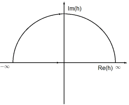
Figure 3:Contour following the complete real axis and than making half a circle over the upper half of the complex h-plane
I1=
1 (1 +δ0n)2π2λ
Z ∞
−∞
dhexp [ih(z−z0)]
(λ2+h2−k2)
n2
rr0
Jn(λr)Jn(λr0)
cos
sin (nφ) cos
sin (nφ0) ˆrrˆ0
+∂
∂rJn(λr) ∂ ∂r0
Jn(λr0)
sin cos (nφ)
sin
cos (nφ0) ˆφ ˆ
φ0
∓n rJn(λr)
∂ ∂r0
Jn(λr0)
cos sin (nφ)
sin
cos (nφ0) ˆr ˆ
φ0∓
n r0
Jn(λr0)
∂
∂rJn(λr)
cos sin (nφ0)
sin
cos (nφ) ˆr0 ˆ
φ !
= f1
(1 +δ0)2π2λ
Z ∞
−∞
dhexp [ih(z−z0)]
(λ2+h2−k2). (138)
Then we rewrite the equation to highlight the poles as follows I1=
f1
(1 +δ0n)2π2λ
Z ∞
−∞
dh exp [ih(z−z0)] h−√k2−λ2
h+√k2−λ2. (139)
The above integral can be solved by the contour integration approach in complex plane. Forz > z0
we integrate over the upper half of the complex plane, as can be seen in Fig. (3). Identifying the poles ath=±√k2−λ2, withk∈C, and then using the residue theorem we get forz > z
0
I1=
f1
(1 +δ0n)2π2λ
2πiexp
i√k2−λ2(z−z 0)
2√k2−λ2 , (140)
I1=
f1
(1 +δ0n)πλ
iexp
i√k2−λ2(z−z 0)
2√k2−λ2 (141)
and finally after working out the coefficients
I1=
iM(√k2−λ2)M 0(−
√
k2−λ2)
2(1 +δ0n)πλ
√
k2−λ2 . (142)
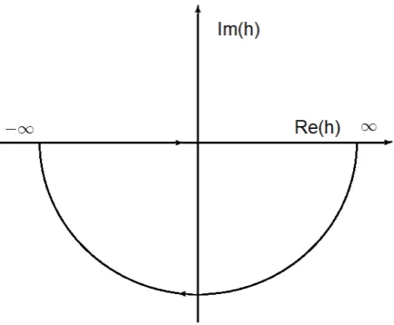
We can repeat the procedure forz < z0by carrying out the integration in the lower half of the complex
plane as seen in fig. (4) . This gives
I1=
f1
iexp
−i√k2−λ2(z−z 0)
Figure 4:Contour following the complete real axis and then making half a circle over the lower half of the complex h-plane
or after once more working out the coefficients.
I1=
iM(−√k2−λ2)M 0(
√
k2−λ2)
2(1 +δ0n)πλ
√
k2−λ2 . (144)
B.2 Second integral
Continuing with the second integral, which is a part of Eqs. (38) and (39),
I2=
Z ∞
−∞
dh N(h)N0(−h)
(1 +δ0n)2π2λ(λ2+h2−k2)
. (145)
After filling in the definition forNfrom Eq. (22) and collecting the prefactors into the coefficientsf1,
I2=
1 (1 +δ0n)2π2λ
∂ ∂rJn(λr)
∂ ∂r0
Jn(λr0)
sin cos (nφ)
sin
cos (nφ0) ˆrˆr0
+n
2
rr0
Jn(λr)Jn(λr0)
cos sin (nφ)
cos
sin (nφ0) ˆφ ˆ
φ0±
∂ ∂rJn(λr)
n r0
Jn(λr0)
sin cos (nφ)
cos
sin (nφ0) ˆr ˆ
φ0
± ∂ ∂r0
Jn(λr0)
n rJn(λr)
sin cos (nφ0)
cos
sin (nφ) ˆr0 ˆ
φ !
Z ∞
−∞
dhexp[ih(z−z0)]h
2
κ2(λ2+h2−k2)
+ λ4Jn(λr)Jn(λr0)
sin cos (nφ)
sin
cos (nφ0) ˆzzˆ0
! Z ∞
−∞
dh exp[ih(z−z0)] κ2(λ2+h2−k2)
!
+ iλ2 ∂
∂rJn(λr)Jn(λr0)
sin
cos (nφ) sin
cos (nφ0) ˆrzˆ0
−iλ2 ∂ ∂r0
Jn(λr0)Jn(λr)
sin
cos (nφ0) sin
cos (nφ) ˆr0zˆ±iλ
2n
rJn(λr)Jn(λr0)
cos
sin (nφ) sin
cos (nφ0) ˆφzˆ0
∓iλ2n r0
Jn(λr)Jn(λr0)
cos
sin (nφ0) sin
cos (nφ) ˆφ0zˆ
! Z ∞
−∞
dhexp[ih(z−z0)]h κ2(λ2+h2−k2)
= 1
(1 +δ0n)2π2λ
f1
Z ∞
−∞
dhexp[ih(z−z0)]h
2
κ2(λ2+h2−k2)+f2
Z ∞
−∞
dh exp[ih(z−z0)] κ2(λ2+h2−k2)
+f3
Z ∞
−∞
dhexp[ih(z−z0)]h κ2(λ2+h2−k2)
. (146)
After rewriting to highlight the poles
I2=
1 (1 +δ0n)2π2λ
f1
Z ∞
−∞
dh exp[ih(z−z0)]h
2
κ2 h−√k2−λ2
h+√k2−λ2
+f2
Z ∞
−∞
dh exp[ih(z−z0)] κ2 h−√k2−λ2
h+√k2−λ2+f3 Z ∞
−∞
dh exp[ih(z−z0)]h κ2 h−√k2−λ2
h+√k2−λ2 !
.
(147) The above integral can be solved similar to the first integral. Identifying the poles ath=±√k2−λ2
andh=±iλwe get forz > z0
I2=
i
(1 +δ0n)πλ
f1
exp[i√k2−λ2(z−z
0)](k2−λ2)
k2 2√k2−λ2 +
exp[−λ(z−z0)]λ2
2iλk2
!
+
f2
exp[i√k2−λ2(z−z 0)]
k2 2√k2−λ2 +
exp[−λ(z−z0)]
−2iλk2
!
+
f3
exp[i√k2−λ2(z−z 0)]
√ k2−λ2
k2 2√k2−λ2 +
iλexp[−λ(z−z0)]
−2iλk2
!!
, (148)
or
I2=
iN √k2−λ2 N0 −
√
k2−λ2
2(1 +δ0n)πλ
√
k2−λ2 +f1
exp[−λ(z−z0)]
2k2(1 +δ 0n)π
−f2
exp[−λ(z−z0)]
2λ2k2(1 +δ 0n)π
−f3
iexp[−λ(z−z0)]
2λk2(1 +δ 0n)π
,
with
GA+=exp[−λ(z−z0)] 2k2(1 +δ
0n)π
∂
∂rJn(λr) ∂ ∂r0
Jn(λr0)
sin cos (nφ)
sin
cos (nφ0) ˆrrˆ0
+n
2
rr0
Jn(λr)Jn(λr0)
cos
sin (nφ) cos
sin (nφ0) ˆφ ˆ
φ0 ±
∂ ∂rJn(λr)
n r0
Jn(λr0)
sin
cos (nφ) cos
sin (nφ0) ˆr ˆ
φ0
± ∂ ∂r0
Jn(λr0)
n rJn(λr)
sin
cos (nφ0) cos
sin (nφ) ˆr0 ˆ
φ−λ2Jn(λr)Jn(λr0)
sin
cos (nφ) sin
cos (nφ0) ˆzzˆ0
+λ ∂
∂rJn(λr)Jn(λr0)
sin cos (nφ)
sin
cos (nφ0) ˆrˆz0−λ
∂ ∂r0
Jn(λr0)Jn(λr)
sin cos (nφ0)
sin
cos (nφ) ˆr0zˆ
±iλn
rJn(λr)Jn(λr0)
cos
sin (nφ) sin
cos (nφ0) ˆφzˆ0∓λ
n r0
Jn(λr)Jn(λr0)
cos
sin (nφ0) sin
cos (nφ) ˆφ0zˆ
! (150)
this gives
I2=
iN √k2−λ2 N0 −
√
k2−λ2
2(1 +δ0n)πλ
√
k2−λ2 +
L(iλ)L0(−iλ)
2(1 +δ0n)πk2
(151)
=iN
√
k2−λ2 N0 −
√
k2−λ2
2(1 +δ0n)πλ
√
k2−λ2 +G +
A. (152)
Repeating forz < z0by integrating over the lover half of the complex plane
I2=
iN −√k2−λ2 N0
√
k2−λ2
2(1 +δ0n)πλ
√
k2−λ2 +f1
exp[λ(z−z0)]
2k2(1 +δ 0n)π
−f2
exp[λ(z−z0)]
2λ2k2(1 +δ 0n)π
+f3
iexp[λ(z−z0)]
2λk2(1 +δ 0n)π
, (153) with
GA−= exp[λ(z−z0)] 2k2(1 +δ
0n)π
∂ ∂rJn(λr)
∂ ∂r0
Jn(λr0)
sin cos (nφ)
sin
cos (nφ0) ˆrˆr0
+n
2
rr0
Jn(λr)Jn(λr0)
cos sin (nφ)
cos
sin (nφ0) ˆφ ˆ
φ0 ±
∂ ∂rJn(λr)
n r0
Jn(λr0)
sin cos (nφ)
cos
sin (nφ0) ˆr ˆ
φ0
± ∂ ∂r0
Jn(λr0)
n rJn(λr)
sin cos (nφ0)
cos
sin (nφ) ˆr0 ˆ
φ−λ2Jn(λr)Jn(λr0)
sin cos (nφ)
sin
cos (nφ0) ˆzzˆ0
−λ ∂
∂rJn(λr)Jn(λr0)
sin cos (nφ)
sin
cos (nφ0) ˆrˆz0+λ
∂ ∂r0
Jn(λr0)Jn(λr)
sin cos (nφ0)
sin
cos (nφ) ˆr0zˆ
∓iλn
rJn(λr)Jn(λr0)
cos sin (nφ)
sin
cos (nφ0) ˆφzˆ0±λ
n r0
Jn(λr)Jn(λr0)
cos sin (nφ0)
sin
cos (nφ) ˆφ0zˆ
! (154)
makes
I2=
iN −√k2−λ2 N0
√
k2−λ2
2(1 +δ0n)πλ
√
k2−λ2 +
L(−iλ)L0(iλ)
2(1 +δ0n)πk2
(155) or
I2=
iN −√k2−λ2 N0
√
k2−λ2
2(1 +δ0n)πλ
√
k2−λ2 +G
−
B.3 Third integral
Finally, the third and last of the integrals involving the non-regularized Green’s functions, which is a part of Eqs. (38) and (40)
I3=
Z ∞
−∞
dh −λL(h)L0(−h)
(1 +δ0n)2π2(λ2+h2)k2
. (157)
Substituting the definition ofLfrom Eq. (24) gives us
I3=
−λ k2(1 +δ
0n)2π2
∂ ∂rJn(λr)
∂ ∂r0
Jn(λr0)
sin cos (nφ)
sin
cos (nφ0) ˆrrˆ0
+n
2J
n(λr)Jn(λr0)
rr0
cos
sin (nφ) cos
sin (nφ0) ˆφ ˆ
φ0±
∂ ∂rJn(λr)
n r0
Jn(λr0)
sin
cos (nφ) cos
sin (nφ0) ˆr ˆ
φ0
± ∂ ∂r0
Jn(λr0)
n rJn(λr)
sin
cos (nφ0) cos
sin (nφ) ˆr0 ˆ
φ !
Z ∞
−∞
dhexp[ih(z−z0)]
(h2+λ2)
+ Jn(λr)Jn(λr0)
sin
cos (nφ) sin
cos (nφ0) ˆzzˆ0
! Z ∞
−∞
dhexp[ih(z−z0)]h
2
(h2+λ2)
+ −i∂
∂rJn(λr)J(λr0)
sin cos (nφ)
sin
cos (nφ0) ˆrzˆ0+i
∂ ∂r0
Jn(λr0)J(λr)
sin cos (nφ)
sin
cos (nφ0) ˆr0zˆ
∓in
r Jn(λr)Jn(λr0)
cos sin (nφ)
sin
cos (nφ0) ˆφzˆ0±
in r0
Jn(λr)Jn(λr0)
cos sin (nφ0)
sin
cos (nφ) ˆφ0zˆ
!
Z ∞
−∞
dhexp[ih(z−z0)]h
(h2+λ2)
=
−λ k2(1 +δ
0n)2π2
f1
Z ∞
−∞
dhexp[ih(z−z0)]
(h2+λ2) +f2
Z ∞
−∞
dhexp[ih(z−z0)]h
2
(h2+λ2) +f3
Z ∞
−∞
dhexp[ih(z−z0)]h
(h2+λ2)
.
(158) The above integral can be solved similar to the previous integrals. Identifying the poles ath=±iλ we get forz > z0
I3=
−λi k2(1 +δ
0n)π
f1
exp[−λ(z−z0)]
2iλ +f2
exp[−λ(z−z
0)]λ2
2iλ +
2π
2πiδ(z−z0)
+f3
exp[−λ(z−z0)]iλ
2iλ
,
(159)
I3=
−L(iλ)L0(−iλ)
2(1 +δ0n)πk2
+ −λf2
k2(1 +δ 0n)π
δ(z−z0), (160)
which comes down to
I3=
−L(iλ)L0(−iλ)
2(1 +δ0n)πk2
− λ k2(1 +δ
0n)π
Jn(λr)Jn(λr0)
sin cos (nφ)
sin
cos (nφ0) ˆzzˆ0δ(z−z0). (161)
Repeating forz < z0by integrating over the lower half of the complex plane
I3=
−L(−iλ)L0(iλ)
2(1 +δ0n)πk2
+ −2λif2
k2(1 +δ 0n)
δ(z−z0) (162)
gives
I3=
−L(−iλ)L0(iλ)
2(1 +δ )πk2 −
λ
k2(1 +δ )πJn(λr)Jn(λr0)
sin
cos (nφ) sin