High fidelity rendering on shared computational resources

(1)

University of Warwick institutional repository: http://go.warwick.ac.uk/wrap

A Thesis Submitted for the Degree of PhD at the University of Warwick

http://go.warwick.ac.uk/wrap/4476

This thesis is made available online and is protected by original copyright. Please scroll down to view the document itself.

(2)

High-fidelity Rendering on Shared

Computational Resources

Vibhor Aggarwal

A thesis submitted in partial fulfilment of the requirements for

the degree of

Doctor of Philosophy in Engineering

School of Engineering

(3)

(4)

List of Figures

1.1 High-fidelity rendering examples . . . 2

1.2 A novel fault-tolerant mechanism for high-fidelity rendering . . . . 5

1.3 A sequence of frames rendered interactively . . . 6

2.1 Description of quantities for calculating radiance . . . 12

2.2 The graphics pipeline for rasterisation . . . 15

2.3 Classic ray tracing algorithm . . . 17

2.4 Ray traversal . . . 19

2.5 Path traced image with different number of samples per pixel (SPP) . . . 20

2.6 k-Nearest neighbour algorithm . . . 24

3.1 Grid computing taxonomy . . . 31

3.2 Four-layered hourglass grid architecture . . . 35

4.1 Two-dimensional Halton and Sobol sequences . . . 55

5.1 Irradiance value interpolation . . . 61

5.2 Selection of frames for the first pass . . . 62

5.3 BFM graphs comparing the two approaches. Kalabsha Walk-through animation was calculated on a single processor while the others were computed on the NGS. . . 64

5.4 The portion of the frame used for calculating the BFM graphs. . . 66

6.1 Quasi-random subdivision of an image . . . 71

6.2 Image subdivision techniques and the resultant image in case of faults. . . 73

6.3 Image reconstruction comparison . . . 74

6.4 The pipeline for the straightforward approach. . . 76

6.5 Image subdivision based on components. . . 77

6.6 The pipeline for the component-based approach. . . 78

(8)

6.7 Indirect lighting calculation for the Sibenik model . . . 79

6.8 The scenes used for the experiments . . . 82

6.9 The VDP results. . . 84

6.10 VDP comparison for the Sibenik model . . . 85

6.11 Cornell Box visual comparison . . . 86

6.12 Fault-tolerant nature of the component-based algorithm. . . 87

7.1 The pipeline for interactive rendering on a desktop grid. . . 91

7.2 The overview of the interactive rendering system . . . 93

7.3 The scenes used for evaluation . . . 100

7.4 The comparison of visual quality of an interactive sequence . . . . 101

7.5 A frame of the Race Car interactive sequence rendered on different number of resources. . . 103

7.6 The VDP comparison for frame 70 from the Kiti interactive se-quence. . . 104

7.7 The convergence of visual quality of static images . . . 105

7.8 The efficiency comparisons for rendering on different number of resources. . . 107

7.9 The visual quality comparison of reconstruction methods for in-teractive sequences. . . 108

8.1 The pipeline for the ETPF approach . . . 114

8.2 Three-dimensional Sobol Sampling . . . 115

8.3 The time-constrained pipeline for the MQS approach. . . 115

8.4 The overview of the time-constrained animation rendering system 116 8.5 The description of scenes used for evaluation . . . 118

8.6 The Temporal Fault variation (TF50) . . . 121

8.7 The VDP comparisons for the animations . . . 122

8.8 The VDP comparison for a frame of the Kiti animation . . . 123

8.9 The RMSE comparisons for the animations . . . 124

8.10 Count versus SPP for different frames . . . 126

(9)

List of Tables

4.1 Generation of first 10 numbers of a base-2 van der Corput sequence 49

5.1 Animation Description and Timings . . . 67

6.1 Component-based approach versus straightforward approach . . . 81 7.1 Fixed frame rate used for various scenes. . . 107

8.1 Time-constraints used for various animations . . . 120

8.2 Average RMSE Values . . . 125

(10)

Acknowledgements

This thesis would not have been possible, had Alan not replied to one of the many random emails he gets daily and if Kurt had not instigated me into the intriguing world of research during my undergraduate internship. It is only fitting that both of them jointly supervised me on this thesis. I am highly indebted to them for their constant support and encouragement while enthusiastically motivating me through this journey.

The Visualisation Group at the University of Warwick has been immensely helpful in providing a strong sense of a research community. Both Tom and Piotr provided invaluable assistance during the research, offering useful insights and advice. Vedad and Jass were always present whenever I got stuck. Alena, Alessandro, Belma, Carlo, Ela, Elmedin, Francesco, Gabriela , Jasminka, Matt, Mike, Peter, Remi, Sandro, Silvester, Simon: it was great working with all of you and I especially enjoyed our outings together.

Usama, who tragically passed away in October 2007, deserves a special men-tion. He once showed me how he could do “magic” by reconstructing images from sparse samples and thus inspired me to use these techniques for my research. His ever-smiling face will always be an inspiration.

The thesis writing group: Claire, Jayne, Kim, Rosario and Shaobo, had a crucial role in getting this thesis written. They were always there when I struggled to put words on the paper.

My wonderful experience at Warwick has been enriched by countless number of friends I made here. They have been responsible for providing a truly inter-national environment, exposing me to the multitude of cultures from around the world. Ankit, David, Hardik, Himanshu, Hitesh, Katty, Kavit, Marvin, Marzia, Max, Merve, Mouz, Nagesh, Nur, Prakash, Ramina, Saurin: being so far away from home would not have been so easy without you.

Finally, my parents and family have always supported me tirelessly in all my endeavours. I could not have done this without your affection and kind thoughts! I would like to express my gratitude to all the people, not only just those mentioned above, but numerous others as well who were part of the whole PhD process and assisted me in various ways during the past three years. I am also thankful to the University of Warwick for funding my research through the Vice Chancellor’s scholarship.

(11)

Declaration

The work in this thesis is original and no portion of work referred to here has

been submitted in support of an application for another degree or qualification

of this or any other university or institute of learning.

Signed: Date: 15 October 2010

Vibhor Aggarwal

(12)

List of Publications

The following have been published as a result of the work contained within this

thesis.

Journal paper

• Aggarwal V., Debattista K., Bashford-Rogers T., Dubla P., Chalmers A.: High-fidelity Interactive Rendering on Desktop Grids. IEEE Computer

Graphics and Applications, PrePrints (2010).

Peer-reviewed Conference Papers

• Aggarwal V., Chalmers A., Debattista K.: High-Fidelity Rendering of Animations on the Grid: A Case Study. In Eurographics Symposium on

Parallel Graphics and Visualization (Crete, Greece, 2008), Eurographics

Association.

• Aggarwal V., Debattista K., Dubla P., Bashford-Rogers T., Chalmers A.: Time-constrained High-fidelity Rendering on Local Desktop Grids. In

Eurographics Symposium on Parallel Graphics and Visualization (Munich,

Germany, 2009), Eurographics Association.

Peer-reviewed Poster

• Aggarwal V., Debattista K., Chalmers A.: High-fidelity Rendering using Distributively-controlled Multi-programmed Computing. In TCPP PhD

Fo-rum, IEEE International Parallel and Distributed Processing Symposium

(Rome, Italy, 2009), IEEE Computer Society.

(13)

Abstract

The generation of high-fidelity imagery is a computationally expensive process

and parallel computing has been traditionally employed to alleviate this cost.

However, traditional parallel rendering has been restricted to expensive shared memory or dedicated distributed processors. In contrast, parallel computing on

shared resources such as a computational or a desktop grid, offers a low cost

al-ternative. But, the prevalent rendering systems are currently incapable of

seam-lessly handling such shared resources as they suffer from high latencies, restricted

bandwidth and volatility. A conventional approach of rescheduling failed jobs in

a volatile environment inhibits performance by using redundant computations.

Instead, clever task subdivision along with image reconstruction techniques

pro-vides an unrestrictive fault-tolerance mechanism, which is highly suitable for

high-fidelity rendering. This thesis presents novel fault-tolerant parallel render-ing algorithms for effectively tapprender-ing the enormous inexpensive computational

power provided by shared resources.

A first of its kind system for fully dynamic high-fidelity interactive rendering

on idle resources is presented which is key for providing an immediate feedback

to the changes made by a user. The system achieves interactivity by monitoring

and adapting computations according to run-time variations in the computational

power and employs a spatio-temporal image reconstruction technique for

enhanc-ing the visual fidelity. Furthermore, algorithms described for time-constrained

of-fline rendering of still images and animation sequences, make it possible to deliver the results in a user-defined limit. These novel methods enable the employment

of variable resources in deadline-driven environments.

(14)

(15)

CHAPTER 1

Introduction

In the past few decades, many researchers have been attracted to the field of

high-fidelity rendering in search of techniques which can generate realistic

im-ages of virtual environments quickly and accurately, by exploiting the advances

made in modern computing architectures. Recently, computational platforms

have emerged which are designed for sharing resources between the users. These

platforms allow their users to benefit from increased computational power at a reduced cost by aggregation of resources. This thesis is the first to investigate

the challenges for high-fidelity rendering on such shared computational resources,

and presents novel algorithms to tackle them.

1.1 High-fidelity Rendering

Rendering is the process of digital generation of imagery using the description

of a virtual scene containing information about its geometry, lighting, material properties and camera attributes. This can be classified into two main categories:

photorealistic and non-photorealistic rendering. The former deals with generation

of images which are similar to a real photograph of the scene while the latter

imitates artistic representations such as paintings and cartoons.

High-fidelity rendering uses physically-based quantities for generating

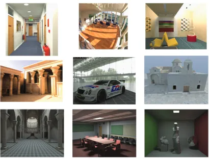
photo-realistic images and is the focus of this thesis, see for example Figure 1.1. This

involves computation of light transport through a virtual scene by simulating

light interactions between the surfaces present in it, thereby determining the

amount of light reaching the camera. A global illumination lighting model is

used such that light interactions between all the surfaces are taken into account for the image generation process, resulting in effects which occur in real world

(16)

[image:16.595.113.524.95.407.2]

1. Introduction 2

Figure 1.1: High-fidelity rendering examples

such as colour bleeding, soft shadows, caustics etc. A mathematical model for the whole process was formulated by Kajiya [Kaj86], known as the rendering

equation. The major challenge lies in solving this equation, due to the associated

computational expense.

1.1.1 Applications

The application of high-fidelity rendering techniques has been restricted due to

their computationally expensive nature. However, the advancements in the

ren-dering techniques and computer hardware, including specialised Graphics

Pro-cessing Units (GPUs), have increased their scope to a great extent as evident

from the following examples [DBB06]:

• Architecture: Architects employ high-fidelity rendering to generate realis-tic images and walk-throughs of building designs [BHWL99, ASKCK03], to

help their clients visualise them under different interior and exterior

(17)

1. Introduction 3

conditions and modify the designs according to the client’s preferences

be-fore the construction starts.

• Archaeology: Many archaeological sites around the world have been dam-aged with time and archaeologists reconstruct them to be able to preserve

and study cultural heritage [HMD∗10]. High-fidelity renderings of virtual reconstructions assist them to view sections of the sites which may not

ex-ist any more. Relighting the cultural heritage sites with authentic lighting

conditions helps them recreate the past with a greater accuracy.

• Visual Effects: The modern movie industry relies heavily on computer gen-erated imagery [TL04,PFHA10]. This allows them to add virtual characters

into a scene or enhance the visual appeal of the scene using special effects.

For these additions to be believable, the lighting conditions used for virtual components need to be similar to that of the real scene and high-fidelity

rendering provides this facility.

• Lighting Design: High-fidelity rendering techniques provide a practical tool for lighting engineers [GGHS03]. It helps them to design and study light

sources and characterise their emission properties by placing them in virtual

environments. They can then verify these findings by conducting physical

measurements.

• Computer Games: For the past few years, the computer games industry has been constantly pushing the limits of the current computer graphics

capabilities to offer gamers an immersive environment by generating ever

more realistic images [Mit07]. Computer games these days are increasingly

using high-fidelity techniques for this, however, due to the computationally

expensive nature of these techniques, they have been usually limited to

pre-rendered visuals.

• Product Design: Product designers also benefit from high-fidelity render-ings. This provides them with a useful tool for enhancing their designs of products such as cars, furniture, appliances, consumer electronics by

simu-lating their appearance under various lighting conditions [RMS∗08,KLN09]. Furthermore, such images can also be used for advertising new products

(18)

1. Introduction 4

• Training Simulators: An accurate visual stimulus enhances the effectiveness of training simulators as it provides the users with a good representation of

real environments, preparing them for scenarios they are likely to encounter in real life. For example, generating precise visuals for different visibility

levels for use in a flight simulator is very important to train the pilots for

adverse weather conditions [Nie03].

High-fidelity rendering allows these applications to study and visualise

real-world scenarios at a much lower cost in a safe and controlled manner. For

ex-ample, physical construction of a building would require much more money and

time than creating a virtual model. Also, modification of a virtual prototype

is a lot more simple than changing a physical entity. Furthermore, it may not

always be feasible to create a real-world alternative. For example, replacement of virtual characters used in movies and recreation of scenarios used for training

simulators. Hence, high-fidelity rendering is crucial for these applications and

any future advancements made in rendering would be beneficial for them.

1.2 Shared Computing Resources

The advances made by the semiconductor industry following Moore’s Law have

led to a considerable increase in computational power of modern day Central Processing Units (CPUs). This has resulted in a widespread use of computers

to solve a multitude of challenges faced by science, engineering and businesses.

However, the computational demands of such applications have continuously

ex-ceeded the processing power of the current generation computers. Hence, parallel

and distributed computing in various shapes and forms have been employed to

address this issue.

Traditional parallel systems have been either shared memory machines

(su-percomputers) or distributed multi-processors connected by high speed networks

(clusters). The high cost of installing and maintaining such systems has restricted

their user base. There is a growing class of applications which process information from a combination of heterogeneous components and they are usually

unsup-ported by such traditional parallel systems. Researchers have been looking to

overcome these problems of cost and heterogeneity by creating mechanisms for

aggregating shared distributed resources across multiple domains. This is known

(19)

1. Introduction 5

Work Subdivision based on Quasi-random

Sampling

Progressive Parallel Rendering using Master-Worker Paradigm

Image Reconstruction

Figure 1.2: A novel fault-tolerant mechanism for high-fidelity rendering which forms the basis of many algorithms presented in this thesis.

grid [FK99]. Grid computing is typically employed to tackle large problems that

can not be solved using resources owned by a single user.

Grid computing inherits the obstacles faced by distributed computing such as

fault-tolerance, synchronisation, communication, heterogeneity, load balancing and scheduling. In addition to these challenges, grid computing needs to tackle

effective sharing and management of distributed resources for a seamless user

experience.

1.3 Rendering on Shared Resources

The computationally expensive nature of high-fidelity rendering has led the

re-searchers to employ parallel computing to alleviate this cost. Many parallel rendering algorithms have been devised exploiting either data parallelism by

de-composing the computations in object space or task parallelism by dede-composing

them in image space [CDR02]. The traditional parallel rendering algorithms

are designed for supercomputers or clusters known as render farms and rely on

quick and frequent communication between the rendering processes. These render

farms are prohibitively expensive, typically costing in excess of £100,000, which

restricts the scope of parallel rendering. Shared computational resources provide

a much cheaper alternative by aggregating idle (already present) resources. But

parallel rendering until now, has not been designed to be fault-tolerant and han-dle run-time variation of resources and hence it is incapable, in any traditional

form, of effectively employing these shared resources.

The conventional fault-tolerance mechanisms for tackling unreliable systems

employ checkpointing or replication or a hybrid of the two approaches. This

results in an extra computational load which limits the performance of algorithms

employing these fault-tolerance strategies. A tradeoff between fault-tolerance and

performance is usually made for computing on shared resources. A novel

(20)

[image:20.595.122.515.101.497.2]

1. Introduction 6

Figure 1.3: A sequence of frames rendered interactively, using the novel fault-tolerance mechanism on volatile resources.

employs quasi-random sequences and image reconstruction techniques without

inhibiting performance, see Figure 1.2.

The variable computational power provided by shared resources makes it

difficult to employ them in a deadline-driven environment. The use of

time-constraints to restrict the computational time is an elegant way of employing

these volatile resources in a production environment where strict deadlines need

to be met. A progressive rendering technique along with the novel fault-tolerant

mechanism allows maximisation of the visual quality of the generated imagery within a given time limit.

(21)

qual-1. Introduction 7

ity imagery to be used as a regular tool in many visualisation applications for

providing an immediate response to the changes made by the user. This would

allow the users to test various parameters of a scene, which is challenging while rendering in an offline environment due to the time involved in such a process.

Interactive rendering requires high-performance computing due to the rate at

which the imagery is calculated and updated. Shared computing resources have

been traditionally used for high-throughput computing. The novel fault-tolerant

mechanism proposed in this thesis enables them to act as a high-performance

resource, as illustrated by the interactively rendered images shown in Figure 1.3.

The generation of high-fidelity animations is a time consuming process even

on render farms, as all individual frames of an animation need to complete before

they can be viewed. An animation studio usually renders multiple drafts of such

animations before finalisation. Time-constrained rendering of such animations on idle resources of an institution would increase their utilisation, while decreasing

the reliance on render farms. Enabling efficient utilisation of existing resources

would help in reducing operational costs, avoiding the need for expensive render

farms.

1.4 Research Objectives

The conjunction of high-fidelity rendering and shared computational resources has been, until now, mostly unexplored. This thesis aims to develop novel

fault-tolerant rendering algorithms for taking advantage of inexpensive shared

resources, building upon the existing knowledge in both the areas of high-fidelity

rendering and shared computational resources. The main research objectives of

this thesis are:

• to develop high-fidelity rendering algorithms with restricted communication to take advantage of massive computational power offered by computational

grids.

• to devise a fault-tolerance mechanism for high-fidelity rendering which does not restrict performance unlike existing fault-tolerance strategies.

(22)

1. Introduction 8

• to create an interactive rendering system capable of handling run-time vari-ations in computational power.

• to develop time-constrained animation rendering algorithms to employ desk-top grids in a production environment.

1.5 Organisation

This thesis is organised as follows:

Chapter 2: High-fidelity Rendering presents an overview of high-fidelity ren-dering and describes the relevant previous work which has been carried out

in this field.

Chapter 3: Computing on Shared Resources covers the background on grid computing and its relevance for high-fidelity rendering.

Chapter 4: Quasi-random Sequences The novel algorithms presented in this thesis rely heavily on quasi-random sequences and this chapter provides a

practical guide on them.

Chapter 5: Animation Rendering on Computational Grids presents and compares two algorithms developed for rendering animations on computa-tional grids and discusses the issues encountered while employing them.

It shows how a two-pass approach can achieve speed-up and better visual

fidelity than existing techniques.

Chapter 6: Time-constrained Offline Rendering on Desktop Grids de-scribes a novel fault tolerant mechanism which uses quasi-random sampling

and image reconstruction techniques. This does not inhibit performance

unlike traditional fault-tolerance strategies. It employs this mechanism for

time-constrained rendering on desktop grids and presents and compares two

algorithms for offline rendering. The advantage of using a component-based approach, by task subdivision at finer granularity, for parallel rendering is

demonstrated.

(23)

1. Introduction 9

on desktop grids. A real-time spatio-temporal image reconstruction

mech-anism is presented which helps in achieving better visual fidelity in the case

of sparse sampling. To the best of the author’s knowledge, this is the first interactive desktop grid system that was developed by creating a new job

scheduling architecture.

Chapter 8: Time-constrained Animation Rendering on Desktop Grids

describes and compares two algorithms developed for rendering

anima-tion with a time-constraint. It shows that an approach based on

multi-dimensional quasi-random sampling has a superior performance than

tra-ditional animation rendering techniques as it progressively refines the whole

animation, even in the presence of faults.

(24)

CHAPTER 2

High-fidelity Rendering

This chapter presents a background on high-fidelity rendering concepts and

algo-rithms while highlighting relevant previous research which has been carried out

in this field. It begins by introducing radiometric quantities to derive the

render-ing equation. Subsequently, three approaches for solvrender-ing the renderrender-ing equation:

rasterisation, radiosity and ray tracing are discussed. Next, a description of

ren-dering techniques used in this thesis is provided. This is followed by an overview of image reconstruction and sparse sampling. Finally, research work carried out

in the areas of time-constrained rendering and parallel rendering is presented.

2.1 Radiometry

The generation of high-fidelity renderings requires computation of light energy

in a scene. Radiometry is a field which studies the measurement of light energy

and hence it is employed for high-fidelity rendering computations. Photometry is another related area of study which deals with perceived brightness of light to

the human eye. The human visual system is not equally sensitive to all the

wave-lengths in the visible spectrum and photometric quantities take this into

consid-eration. However, radiometric quantities are used for high-fidelity rendering and

corresponding photometric quantities can be successively computed [DBB06]. A

description of some radiometric quantities, which are important from the

per-spective of high-fidelity rendering, are presented below following the notations

from [DBB06].

(25)

2. High-fidelity Rendering 11

2.1.1 Radiometric Quantities

2.1.1.1 Radiant Power

This radiometric quantity is useful for estimating the rate of light energy

ema-nating from a light source or reaching a surface. It is also known as flux (Φ) and

is measured in watts, W (joules/sec). Radiant power is independent of the size of source or the surface or the distances between them. A common use of radiant

power is to categorise the light sources, for example a light bulb labelled 100W

transforms approximately 100J of energy every second.

2.1.1.2 Irradiance

Irradiance (E) denotes the radiant power per unit area received on a surface. It is measured in watts/m2.

E = dΦ

dA

2.1.1.3 Radiant Exitance/Radiosity

The amount of radiant power emanating per unit area is termed radiant exitance (M) or radiosity (B). It is also measured in watts/m2_{. The need for defining}

two radiometric quantities to express radiant power per unit area arises since the

incident and exitant light can be potentially different at the same point.

M =B = dΦ

dA

2.1.1.4 Radiance

Radiance is used to measure the amount of light arriving at a point in a given direction. It is the radiant power per unit projected area per unit solid angle

(watts/steradian·m2_{). The projected area refers to the area of the surface}

per-pendicular to the direction. The radiance,L(x→Θ), at a pointxin the direction Θ is given by (see Figure 2.1):

L(x→Θ) = d

2_Φ dωdAcosθ

Radiance is the preferred radiometric quantity for generating high-fidelity

(26)

dA x

Θ

[image:26.595.235.401.97.197.2]

dω

|Θ| = θ

Figure 2.1: Description of quantities for calculating radiance,L(x,Θ), at a point

x in direction Θ, after [DBB06]

appearance of an object [SM09, Jen01]. Furthermore, it is invariant across a line

in space in a vacuum.

The relationships between the radiometric quantities described above can be

defined as:

Φ =

Z

A

Z

Ω

L(x→Θ) cosθdωΘdAx

E(x) =

Z

Ω

L(x←Θ) cosθdωΘ

B(x) =

Z

Ω

L(x→Θ) cosθdωΘ (2.1)

where Ω is the total solid angle and A is the total surface area. L(x → Θ) represents the radiance leaving andL(x←Θ) represents radiance reaching point

x.

2.1.2 Bidirectional Reflectance Distribution Function

The characterisation of surface properties of the materials is needed while

per-forming light transport computations in a scene. When light falls on a surface it

may be absorbed, reflected or transmitted at the same or a different point from the original point of incidence. For example, materials such as marble and human

skin exhibit subsurface scattering phenomenon, that is the light incident on them

gets absorbed and scatters at different points. A Bidirectional Scattering

Sur-face Reflectance Distribution Function (BSSRDF) is defined to model the light

interaction properties of materials. A simpler function, Bidirectional Reflectance

Distribution Function (BRDF), fr, was defined by Nicodemus [Nic65] with the

assumption that light is incident and reflected at the same point, ignoring

sub-surface scattering. BRDF represents the ratio between the radiance reflected in

(27)

is given by:

fr(x,Ψ→Θ) = dLr(x→Θ)

dE(x←Ψ) =

dLr(x→Θ)

L(x←Ψ) cos(Nx,Ψ)dωΨ

(2.2)

where, Nx is the normal vector at x.

Many types of BRDFs have been proposed to model different types of mate-rials such as diffuse, glossy and specular. Kurt and Edwards [KE09] present a

survey of these.

2.2 The Rendering Equation

The equilibrium of light energy in a scene can be mathematically formulated, using the radiometric quantities defined in the previous section, to define the

radiance at any point in that scene. This equation is termed as the rendering

equation [Kaj86] and it forms the basis for high-fidelity rendering algorithms. It

states that the outgoing radiance, L(x → Θ) at a point is equal to the sum of the emitted radiance, Le(x → Θ) and the reflected radiance, Lr(x → Θ) based

on the conservation of energy.

L(x→Θ) =Le(x→Θ) +Lr(x→Θ) (2.3)

Integrating Equation(2.2):

Lr(x→Θ) =

Z

Ωx

fr(x,Θ↔Ψ)L(x←Ψ) cos(Nx,Ψ)dωΨ (2.4)

Substituting in Equation(2.3), to obtain the rendering equation:

L(x→Θ) =Le(x→Θ) +

Z

Ωx

fr(x,Θ↔Ψ)L(x←Ψ) cos(Nx,Ψ)dωΨ (2.5)

This can be also transformed into an area formulation such that the radiance can

be computed by integrating over all the surfaces of a scene represented by set A:

L(x→Θ) =Le(x→Θ) +

Z

A

fr(x,Θ↔Ψ)L(y→ −Ψ)V(x, y)G(x, y)dAy (2.6)

where,

G(x, y) = cos(Nx,Ψ) cos(Ny,−Ψ)

r2 xy

(28)

and V(x, y) represents the visibility term between two points x and y which is 1 if x and y are mutually visible and 0 if not. The above equations assume that the light travels instantaneously through a vacuum and there is no participating media within the scene. Furthermore, they are valid for a single wavelength only

and do not account for phenomena such as diffraction, polarisation and

inter-ference. Modifications to the rendering equation for incorporating participating

media, for example smoke and dust, can be found in [Jen01].

The rendering equation can be classified as second degree Fredholm integral

equation since the quantity to be calculated, radiance, appears on the left hand

side and on the right hand side as part of an integral and it cannot be solved

analytically. There are two approaches to solve the rendering equation: Finite

element methods and point sampling methods. The radiosity approach (see

Sec-tion 2.4) is a finite element method, while rasterisaSec-tion (see SecSec-tion 2.3) and ray tracing based algorithms (see Section 2.5) are point sampling methods for

estimating the rendering equation for a scene. The algorithms proposed in this

thesis are suited for point sampling methods only.

2.3 Rasterisation

There are two major categories of digital image synthesis techniques: object-order

and image-order [SM09]. Object-order methods iterate through each object in the scene for generating images while image-order methods iterate through each

image pixel and find the objects which influence its colour. Rasterisation

tech-niques are object-order methods which map the scene geometry to image pixels

whereas ray tracing based algorithms are image-order methods. Rasterisation has

been brought to the forefront in comparison to ray tracing methods, due to the

support provided by GPUs which implement these techniques in hardware and

APIs such as OpenGL and DirectX. Although lately, with the increased flexibility

of GPU programming, ray tracing methods [PBD∗10] have also been developed for exploiting the performance boost provided by the GPU.

Rasterisation has been the popular technique for generating interactive visuals

due to its speed. However, as it does not natively handle global illumination

effects, generation of realistic images is difficult. It approximates effects such as

shadows, reflections and refractions which ray tracing techniques can calculate

(29)

Display

Application Geometry Rasterisation

Figure 2.2: The graphics pipeline for rasterisation, after [AMHH09]

as it deals with polygons, in contrast to ray tracing which is not bound by such

a requirement.

The graphics pipeline for generating images using rasterisation can be broadly

classified into three stages [AMHH09]: application, geometry and rasterisation

(see Figure 2.2), where each of these stages can be further decomposed. The

application stage is responsible for the generation of primitives which need to be

displayed. The geometry stage performs various operations on these primitives

such as modelling transformations, per-vertex illumination, viewing

transforma-tions, clipping and projection before they can be rasterised. The process of rasterisation can be broken into three main subtasks [FvDFH97]: visible

sur-face determination, scan conversion and shading. First, it identifies the polygons

which are visible from the current camera view, then it determines the pixels

which are covered by the visible polygon and finally it colours the pixels based on

a shading algorithm. A plethora of techniques exist for accelerating rasterisation

while increasing the degree of realism such as texture filtering, bump mapping,

environment mapping, level of detail, shadow volumes etc. and an overview of

these can be found in [AMHH09].

2.4 Radiosity

Radiosity methods provide a view-independent approach for computing light

transport in a scene using finite element methods. Goral et al. [GTGB84]

de-scribed the classical radiosity approach which discretised the scene geometry and

computed radiosity for each patch of the surface geometry by solving a system

of linear equations. All the surfaces in the scene were considered to be diffuse,

hence the radiance and the BRDF were only dependent on the position.

Rewrit-ing Equation(2.6) as:

L(x) = Le(x) +ρ(x)

Z

A

(30)

where ρ(x) represents the BRDF. Also, B(x) = πL(x) and Be(x) = πLe(x) for

diffuse environments. Therefore:

B(x) =Be(x) + ρ(x)

π

Z

A

B(y)V(x, y)G(x, y)dAy

This radiosity equation can be solved by a summation over the patches, using

a system of linear equations to compute radiosity, Bi, for each patch of the

discretised geometry as:

Bi =Bei+ρi

X

j

FijBj

whereFij refers to the form factor between two patches which defines the fraction

of power arriving from one patch to the other. The classical radiosity approach

first discretises the geometry, calculates the form factors and then solves the system of linear equations using Jacobi or Gauss-Seidel iterations. The two major

issues with this approach lie in geometry discretisation and form factor calculation

and storage [DBB06]. Research has been carried out to tackle these issues and a

review of other approaches can be found in [DBB06, CW93].

The major advantage of computing light transport using radiosity is that it

is view-independent and once it has been computed it can be used to generate

interactive walk-throughs. Also, form factor calculations can be reused in case of

static scenes with dynamic lighting. However, the major disadvantage of radiosity

is that it is only applicable for scenes with diffuse surfaces. Algorithms have been developed to incorporate non-diffuse surfaces, for example [ICG86, SP89,

SAWG91, AH93], but they usually try to estimate both rendering and radiosity

equations, making them computationally expensive.

2.5 Ray Tracing

Ray tracing is a popular technique for generating high-fidelity images which

com-putes the inter-reflections of light around a scene to simulate the light transport.

It is an image-order rendering approach [SM09], whereby objects in a scene that are needed for shading computations of a pixel are identified for each pixel of the

image to determine its colour value. A light ray is usually traced in a direction

opposite to which the light travels, that is from the viewpoint to the light source

and hence it is also termed a camera or an eye ray. This is done to prevent

(31)

Image Plane Viewpoint

Light Source

Shadow Rays

Camera Rays

Reflected Ray

Figure 2.3: Classic ray tracing algorithm

terminate at the viewpoint.

The first ray tracing approach in computer graphics is attributed to Appel

[App68] who shot one ray for each pixel to determine the closest intersecting object in the scene for visible surface detection. This approach is known as ray

casting and is the simplest form of ray tracing, as it does not propagate the light

rays after the first intersection. When light falls on a surface it may be absorbed,

transmitted or reflected depending on the surface properties of the material. The

classic ray tracing approach [Whi80] on the other hand, simulates the interaction

of light with object surfaces by shooting reflected or transmitted rays, recursively

upon intersection with a specular surface. Also, at each diffuse intersection point,

a shadow ray is shot towards the light source to determine if a point is in shadow.

If the shadow ray intersects another object before hitting the light source then the point is considered in the shadow (see Figure 2.3). The classic ray tracing

approach is also termed Whitted-style ray tracing.

A basic ray tracer consists of three components [SM09]: ray generation, ray

intersection and shading. The first component generates the rays at various steps

of the process. The second determines the closest object which intersects with

the generated ray. Finally, the last component calculates the pixel colour using

(32)

2.6 Point Sampling Methods

Many algorithms with different sampling strategies have been proposed to

gener-ate high-fidelity images using point sampling methods, for example: distributed

ray tracing [CPC84], path tracing [Kaj86], bi-directional path tracing [LW93],

Metropolis light transport [VG97], photon mapping [Jen96], irradiance caching

[WRC88], instant radiosity [Kel97], instant global illumination [WKB∗02] etc. This section provides an overview of the rendering algorithms which are

impor-tant from the perspective of this thesis. An overview of the other algorithms can

be found in [DBB06].

2.6.1 Distributed Ray Tracing

The classical ray tracing approach generates unnatural images due to the fact

that the algorithm supports only point light sources and ideal specular reflection or transmission. This gives rise to artefacts such as hard shadows and mirror-like

reflections and does not account for realistic phenomena such as soft shadows,

glossy reflections, depth of field, motion blur etc. This limitation in the generation

of ray direction was overcome by Cook et al. [CPC84], who accounted for all these

subtleties in the light interactions by stochastic sampling, which generated

high-fidelity images. Their algorithm is also known as distributed ray tracing.

The distributed ray tracing algorithm employs the Monte Carlo integration

technique to estimate the rendering equation. Monte Carlo methods estimate an

integral by randomly sampling the function repeatedly and then averaging the results. The larger the number of samples used, the more accurate the estimation.

Mathematically, if:

I =

Z

D

f(x)dx

thenI can be estimated by drawing outN random samples ofxfrom the domain

D using Monte Carlo integration as:

hIi= 1

N N

X

i=1 f(xi) p(xi)

(33)

Ap-2. High-fidelity Rendering 19

plying Monte Carlo integration principle to estimate the rendering equation; the

reflected radiance,Lr(x→Θ) (from Equation(2.4))can be estimated as [DBB06]:

hLr(x→Θ)i=

1

N N

X

i=1

fr(x,Θ↔Ψi)L(x←Ψi) cos(Nx,Ψi) p(Ψi)

by selectingN random directions, Ψi, with probabilityp(Ψi) over the hemisphere

Ωx. However, the incoming radianceL(x←Ψi) needs to be evaluated. For this,

a ray is traced in direction−Ψi to estimate the incoming radiance, also known as

indirect illumination if the ray does not hit a light source directly. This process

is repeated recursively and results in a ray explosion. To curtail the size of the

tree, termination conditions such as maximum depth or Russian roulette are employed [DBB06]. The shadow rays are generated at each hit point, similar

to the classical ray tracing approach. However, the direction of shadow rays

is chosen by sampling different points on the light surface to estimate what is

termed as the direct illumination. The process of averaging the radiance using

multiple shadow rays accounts for soft shadows.

The variance in the incoming radiance from the different randomly sampled

directions gives rise to noise in the resultant image. This high frequency noise

is minimised by increasing the number of samples which translates into shooting

more rays into the scene at each point. This makes the process computation-ally expensive for generating high-fidelity images using Monte Carlo techniques

and researchers in the field have focussed their efforts at reducing the noise and

accelerating the process.

Objects Lights

(a) Distributed Ray Tracing

Objects Lights

(b) Path Tracing

(34)

(a) 10 SPP (b) 100 SPP

[image:34.595.118.520.108.437.2]

(c) 1,000 SPP (d) 10,000 SPP

Figure 2.5: Path traced image with different number of samples per pixel (SPP)

2.6.2 Path Tracing

Path tracing is one of the simplest high-fidelity rendering algorithms, introduced

by Kajiya [Kaj86]. The distributed ray tracing approach can be considered as an

inorder traversal of the tree of rays generated in a scene, while path tracing

re-peatedly traverses a random path from the root to a leaf node, see Figure 2.4. At

each hit point, rather than sampling N random directions as in distributed path tracing, only one direction is sampled for path tracing which prevents a ray

explo-sion and reduces memory requirements. Each path gives a crude approximation of the incoming radiance but averaging many such paths gives a good estimate

of the radiance value for each pixel. Furthermore, every path is a Markov Chain

through the scene which can be terminated based on criteria similar to those used

for limiting the tree depth in distributed ray tracing. A pixel represents a small

area of the image and by shooting paths through different points in the pixel area

(35)

is that it does not employ any optimisations for calculating the light transport

and hence it is computationally expensive for obtaining noise-free images. As an

example, Figure 2.5 shows the convergence of a path traced image with varying samples per pixel. This algorithm is widely used for generating reference images

to compare with other algorithms due to its simplicity and correctness.

2.6.3 Irradiance Caching

Traditionally, in a distributed ray tracing system, a large number of rays are shot

at each ray intersection point to sample incoming radiance from the hemisphere

around that point. Ward et al. [WRC88], observed that the indirect diffuse

component in a scene is a continuous function in space over the surface of an

object and unlike specular or highly glossy components, it is not subject to high

frequency variations. To exploit this nature of the rendering computation, they

proposed an acceleration data structure to store the world space irradiance values

computed in the scene. Whenever a new irradiance sample is needed, the cache is consulted to check if there is another sample already calculated in the cache

within the user-specified error metric. If there exists such a sample in the cache,

the sample to be calculated is interpolated from it, preventing generation of

additional rays which would otherwise be traced. The authors show that this

strategy of reusing computations provides an order of magnitude speed-up over

traditional methods.

The irradiance cache samples are stored in an octree data structure which

accelerates the search process for selecting relevant samples. Irradiance gradients

[WH92] are employed to choose cached samples which provide a good estimate of the irradiance. Each sample is weighed according to the given formula:

wi(P) =

1

||P−Pi||

Ri +

p

1−NP ·NPi

wherewi(P) represents the weight of the cache samplePifor estimating irradiance

at point P. Ri refers to the mean harmonic distance of the visible objects from Pi and NP denotes the surface normal at P. It can be observed that the larger

the distance to the cached sample, the lower the weight assigned to it. Also,

smaller weight is used for samples whose surface orientation differs significantly.

(36)

The advantages of using irradiance caching are that it is independent of the

geometry and as opposed to other methods such as photon mapping and radiosity

it is view-driven, conforming to the more traditional ray tracing approach of computing from the point of view of the camera. With a view-driven approach,

a walk-through animation path may visit only certain parts of the model being

rendered and since this is known beforehand, only those values which are required

are computed rather than computing global illumination for the whole model.

Moreover, irradiance caching is an established method used in film production

[TL04, Her04] and there are many other algorithms based on irradiance caching

[TL04, AFO05], adaptations used for dynamic scenes [TMD∗04, SKDM05] and adaptive versions of it [YPG01, KBPv06, Deb06, DCG∗07]. Yet others perform similar approaches to compute rendering features, such as participating media

[JDZJ07], glossy interreflections [KGPB05] and subsurface scattering [KLC06].

2.6.4 Instant Radiosity

Keller [Kel97] proposed a two-pass algorithm for calculating the light transport in

a scene. In the first pass of the algorithm, photons are traced from the light source

similar to photon mapping or bidirectional path tracing. They are deposited on

non-specular surfaces of the scene and act as light sources, termed Virtual Point

Lights (VPLs), in the second pass of the algorithm. A GPU is then employed

to generate images for each VPL with shadows and the resultant images are

averaged to obtain the final image.

Wald et al. [WKB∗02] extended this idea for computing global illumination interactively using parallel machines. In the second pass instead of using raster-isation, ray tracing was employed and the VPLs were sampled with shadow rays

for estimating the indirect illumination. They used interleaved sampling and

fil-tering techniques to reduce the computational costs. The complete set of VPLs

was divided into groups of VPLs and each pixel in a tile used a different group

of VPLs to approximate the lighting. The resultant image was filtered using a

discontinuity buffer to generate the final image. The advantage of using VPLs

for approximating the indirect lighting is that the high frequency noise observed

in path tracing type methods is eliminated, resulting in smoother images in less

(37)

2.7 Sparse Sampling and Image Reconstruction

The generation of high-fidelity images using the algorithms described before is a

computationally expensive process and research has focused on reducing this cost.

An important property of such imagery is its spatial and temporal coherence, that

is pixels of an image which are close in space and time are highly correlated. This

characteristic of an image can be exploited to reduce the computation by sparsely

sampling the image and then using image reconstruction techniques to interpolate

the missing pixels. This idea has been widely used for generating high-fidelity

images in reasonable times. Quasi-random sequences (see Chapter 4) have been

typically used for approximating the solution to the rendering equation by sparse sampling, and Shirley et al. [SEB08] provide an overview of such techniques.

However, the primary purpose of employing these sequences in this thesis is to

enable fault-tolerant rendering.

2.7.1 Image Reconstruction Techniques

Image reconstruction refers to the process of estimating missing pixels from a

set of given pixels in order to complete the image. There are many techniques

for reconstructing image pixels and they can be classified into global and local

methods. Global methods utilise all the samples present in an image for

inter-polating the missing pixels.Estimation using local methods is influenced only by

samples near the missing pixel. Global methods can be only applied to smaller

data sets due to the amount of computational complexity. On the other hand, local methods can be used for reconstruction of larger data sets.

One of the widely used local methods is the nearest neighbour algorithm

[Ban09]. In the simplest form, the value of a valid sample, closest to the pixel

being estimated, is copied to reconstruct the image. Other variations interpolate

the value using k-nearest neighbours, that is they find k closest valid pixels and estimate using different interpolation functions. Figure 2.6 shows an example of

k-nearest neighbour algorithm; the black pixels depict valid samples, the grey pixels denote missing samples and the red pixel is the one being reconstructed.

The valid pixels inside the dotted circle are used for reconstructing the pixel value.

A variety of functions have been proposed and used for interpolating from k

(38)

[image:38.595.233.403.96.266.2]

Figure 2.6: k-Nearest neighbour algorithm

uses weighted average, such that farther pixels are assigned lower weights based on

the idea that the influence of a sample decreases with distance. The reconstructed

value, s(p) of pixel, p using k valid pixels, pi with values, fi is given by:

s(p) =

k

X

i=1

wi(pi)∗fi

where weight, wi(pi) is defined as:

wi(pi) =

hi(pi)

Pk

i=1hi(pi)

and hi(pi) varies with inverse Euclidean distance, d(pi) betweenpi and p:

hi(pi) =

1 [d(pi)]α

such that α > 1. Other functions, such as Radial Basis Function [MDH07], polynomial spline [Doo76] etc. have also been employed for interpolation of

two-dimensional data sets. They may offer better interpolation, but they are usually

more computationally expensive requiring at least a few seconds to compute

[MDH07].

While reconstructing using k-nearest neighbours, care must be taken not to interpolate across edges as this leads to generation of visual artefacts. Bilateral filtering [TM98] is commonly employed to preserve edges while filtering an image.

(39)

it with a spatial filter, which for image reconstruction can bek-nearest neighbour. Recently a class of algorithms has been developed, [CPD07, AGDL09, ABD10]

which accelerate bilateral filtering by using a multi-dimensional representation of the image. Colour values are also represented as distinct dimensions, in addition

to the spatial dimensions. This class of algorithms uses a splat-blur-slice approach

to accelerate bilateral filtering, where the multi-dimensional data is projected to

a low-resolution spatial data structure, then a Gaussian blur is performed and

finally the data is sampled at the original positions.

2.7.2 Sparse Sampling

The generation of interactive visuals has traditionally followed a double-buffering

approach, that is two buffers are used for displaying interactive renderings. The

front buffer contains the image which is displayed on the user screen and the next

image to be displayed is rendered in a back buffer. Once rendering finishes, the

back and the front buffers are swapped. This model restricts the interactivity of the system as the minimum time between frames is the amount it takes to render

a full frame. For high-fidelity rendering, this imposes a severe constraint and

hence the idea of sparse sampling has been successfully employed to overcome

this issue. This was first proposed by Bishop et al. [BFMZ94] in the form of

Frameless Rendering. Their idea was to compute a fraction of the frame using a

highly simplified version of Cook’s distributed ray tracer [CPC84]. They rendered

a randomised set of pixels, between screen updates using the latest parameters

for rendering, to prevent image tearing, and a simultaneous partial update of the

full image. In the transient state, this appeared as motion blur and when a stable state was achieved, the image was eventually fully rendered.

The idea of Frameless Rendering was further improved by the Render Cache

algorithm [WDP99]. It stores every sample generated from the ray tracing engine

into a data structure containing information about the hit point, colour and its

age. These samples are reprojected onto the current view and depth information

is used for occlusion. Any holes in the resulting image are filled by using linear

interpolation and filtering. Also, new samples are recalculated after they age

be-yond a particular threshold. Heuristics are employed to prematurely age samples

which are in the areas most likely to change, hence offering a progressive refine-ment of the view. The rendering process is decoupled from the viewing process

(40)

with quick changes and the transient images show visible artefacts. Walter et

al. proposed an improved version of the Render Cache algorithm [WDG02] by

adding an additional filtering pass and lowering the visual artefacts by employ-ing predictive samplemploy-ing. Furthermore, they optimised the algorithm for coherent

memory access to gain speedup. Other similar techniques have been presented

by Ward and Simmons [WS99], and Simmons and S´equin [SS00].

The Render Cache methods used image-based techniques for interpolating

from sparse samples. Tole et al. [TPWG02] improved on this idea by performing

reconstruction in the object space using a Shading Cache. Their data structure

stored the samples on the scene geometry and used GPU for interpolating

miss-ing samples. This helped in limitmiss-ing the visual artefacts, however it took time

to update global illumination effects in dynamic scenes with moving lights and

objects. Bala et al. [BWG03] extended the Shading Cache by preserving dis-continuities during the image reconstruction process. They determined object

silhouettes and shadow edges in real-time and prevented reconstruction across

these boundaries for a better visual fidelity. These algorithms have been

im-plemented and enhanced using the advanced flexibility provided by modern day

GPUs and presented in [VALBW06, SaLY∗08].

Dayal et al. [DWWL05] presented ideas to optimise the process of generation

of new samples and the reuse of older samples in the form of Adaptive Frameless

Rendering. They used a guidance mechanism to adaptively generate new

sam-ples based on spatio-temporal colour variations. Furthermore, they employed filtering in temporal domain based on temporal gradients and implemented the

reconstruction process on GPU. All the methods described above provide a

sub-stantial gain while presenting visual feedback to a user, however they suffer from

distracting artefacts such as image tearing, missing pixels etc.

Adaptive or progressive rendering techniques, for example [BFGS86, Mit87,

PS89, LWC∗02], are also similar to sparse sampling methods. These compute a coarse approximation of the rendered image and then refine it over time. While

using such algorithms in a double-buffering approach, it is very important to

decide when to switch between the buffers. Woolley et al. [WLW02] presented a scheme for making this decision, which they termed interruptible rendering. The

idea was to continue the rendering process until the temporal error exceeds the

spatial error. The temporal error refers to the error which is the result of time it

takes for the computation of an update from when the user triggered it and the

(41)

2.8 Time-constrained Rendering

Rendering systems have often been subjected to time-constraints due to the

var-ious possibilities of continually adapting and refining the computation. The use

of time-constraints thus allows algorithms to be designed such that they aim

to achieve the best possible quality within a given time period. These become

extremely useful in the case of interactive rendering, where screen updates are

generally required at a fixed rate to maintain smooth interactivity.

Funkhouser and S´equin [FS93] devised a mechanism for rendering models

interactively using rasterisation at a fixed frame rate. The models in the scene

were pre-processed at discrete level of detail and their greedy algorithm predicted which version to render in order to maintain the time-constraint. This was done

to maximise the benefit obtained by rendering at a particular level of detail,

such that the cost associated with rendering at that refinement was less than

the constraint. Maciel and Shirley [MS95], and Mason and Blake [MB97] further

extended this idea by creating a single hierarchy of all the objects rather than

treating each object individually and used variations of multiple choice

knap-sack problem for selecting the appropriate representation. Gobbetti and

Bou-vier [GB99] enhanced this approach by using continuous level of detail models.

Zach et al. [ZMK02] presented an algorithm which incorporated both continuous

and discrete level of detail for rendering of terrains at a guaranteed frame rate using polygonal and point-based rendering. An importance metric was presented

by Gao et al. [GLH∗08] for distributed visualisation of large data sets to deter-mine the rendering order and the level of detail for a block of data set based on

view-dependent, application-dependent and data-dependent criteria.

Reisman et al. [RGS00] used time-constraints for interactive parallel ray

trac-ing. They used a progressive sampling strategy based on Delaunay triangulation

while treating the image plane as a continuous space. They refined their solution

until a given deadline and then reconstructed the image from calculated samples

using piecewise linear interpolation. Debattista et al. [DSSC05] provided a frame-work for controlling the pixel quality in a time-constrained setting for generation

of high-fidelity images without perceivable difference. They proposed a regular

expression to specify the pixel computations based on different components.

De-battista [Deb06] further enhanced the approach by using time-constraints with a

(42)

2.9 Parallel Rendering

The large computational complexity exhibited by high-fidelity rendering has

en-couraged researchers to tackle the rendering problem with parallel computing.

An early survey of parallel rendering techniques and related issues is provided

by Crockett [Cro97]. A detailed survey of these methods especially in context of

global illumination and ray tracing is presented by Chalmers et al. [CDR02]. Ray

tracing algorithms are relatively easy to parallelise if the entire scene description

can be duplicated on each processor, as each processor can be designated to

in-dependently work on a part of the image-space. However, load balancing can be

challenging.

Parallel rendering tasks can be constructed by subdividing either in

image-space or object-image-space. The former is suitable if the scene data can be replicated on

each processor and the latter is generally used when the scene data is larger than

the memory size of an individual processor. A uniform load balancing is easier

to achieve with image-space subdivision (for example [Woo84, PB85, LS91]) but

it leads to poor memory usage. In contrast, a scene can be distributed evenly

using object-space subdivision (for example [DS84, PB89, Pit93]) but it results

in complex load balancing strategies. Many algorithms have been proposed in

both categories taking advantage of hardware and application environments. A

hybrid task subdivision strategy was developed independently by Salmon and Goldsmith [SG88], and Scherson and Caspary [SC88], where object data is

hi-erarchically subdivided. The upper portion of this hierarchy is replicated on all

processors while the lower part with most of the scene data is distributed allowing

dissociation of image-space and object-space.

Load balancing can be static or dynamic based on the scheduling policy

adopted by the algorithm. Heirich and Arvo [HA98] provided a good comparison

of various load balancing techniques and showed that any static task subdivision

strategy is affected by load imbalances. In their experiments, they observed that

a hybrid method reduced the load imbalance cost such that it was smaller than other costs of parallelisation. Badouel and Priol [BP89] described a dynamic

demand-driven load balancing based on the master-worker paradigm whereby

each worker is assigned a 3×3 tile of pixels when it becomes idle. But this ap-proach suffered from poor scalability and therefore, Green and Paddon [GP90]

used a hierarchical approach to overcome this. They connected the distributed

(43)

the tree and all the other workers would communicate with their parents only,

limiting the number of requests being sent across the network. This resulted

in better scalability. Reisman et al. [RGS00] devised a dynamic load balancing strategy for progressive ray tracing on distributed clusters exploiting temporal

coherence for obtaining interactive rates. The image was subdivided into regions

which were assigned to separate processors and during run-time the regions were

dynamically adjusted to rectify load imbalances.

One of the first parallel architectures designed for interactive ray tracing

us-ing a 96-processor supercomputer was proposed by Muuss [Muu95]. He needed

interactive rendering for radar systems which had been modelled using large

number of Constructive Solid Geometry (CSG) primitives. These could not be

rasterised as the tessellation of the primitives would have resulted in several

mil-lion polygons. Using traditional ray tracing the author was able to render the CSG primitives directly, preventing the memory and time costs of tessellation.

Keates and Hubbold [KH95] presented an interactive ray tracing system based

on a virtual shared-memory machine which took advantage of cache coherence

by using regular gridcells. Dynamic load balancing was achieved with thread

synchronisation mechanisms to achieve interactivity on 64 processors.

Another such rendering system was proposed by Parker et al. [PMS∗99] using an optimised static load balancing approach. This supported image-based

ren-dering with realistic shadows which also ran on a shared-memory supercomputer.

Interactivity was achieved by designing the jobs to match the caching granular-ity and exploiting fast synchronisation available on the target hardware. They

were also able to perform volume rendering [PPL∗99] and iso-surface visualisa-tion [PSL∗98] using their system which supported frameless rendering in addition to synchronous operation.

Wald et al. [WSBW01] enhanced the methods presented in [PMS∗99] by using object dataflow strategy to run on a distributed cluster. Using a highly optimised

SIMD code they were able to achieve interactivity. Wald et al. [WKB∗02,BWS03] further enhanced this by adding global illumination and handling a few dynamic

scene changes by modifying instant radiosity (see Section 2.6.4).

Purcell et al. [PBMH02] exploited the programmability of the modern GPU

and used it as an efficient and massively parallel stream processor for ray tracing,

demonstrating similar performance to the optimised CPU version of Wald et

High fidelity rendering on shared computational resources

High-fidelity Rendering on Shared

Computational Resources

Vibhor Aggarwal

Contents

List of Figures

List of Tables

Acknowledgements

Declaration

List of Publications

Journal paper

Peer-reviewed Conference Papers

Peer-reviewed Poster

Abstract

CHAPTER 1

Introduction

1.1

High-fidelity Rendering

1.1.1

Applications

1.2

Shared Computing Resources

1.3

Rendering on Shared Resources

1.4

Research Objectives

1.5

Organisation

CHAPTER 2

High-fidelity Rendering

2.1

Radiometry

2.1.1

Radiometric Quantities

2.1.2

Bidirectional Reflectance Distribution Function

2.2

The Rendering Equation

2.3

Rasterisation

2.4

Radiosity

2.5

Ray Tracing

2.6

Point Sampling Methods

2.6.1

Distributed Ray Tracing

2.6.2

Path Tracing

2.6.3

Irradiance Caching

2.6.4

Instant Radiosity

2.7

Sparse Sampling and Image Reconstruction

2.7.1

Image Reconstruction Techniques

2.7.2

Sparse Sampling

2.8

Time-constrained Rendering

2.9

Parallel Rendering