warwick.ac.uk/lib-publications
Original citation:
Ratcliff, Laura E., Hine, Nicholas and Haynes, Peter D.. (2011) Calculating optical absorption
spectra for large systems using linear-scaling density functional theory. Physical Review B
(Condensed Matter and Materials Physics), 84 (16). 165131.
Permanent WRAP URL:
http://wrap.warwick.ac.uk/78155
Copyright and reuse:
The Warwick Research Archive Portal (WRAP) makes this work by researchers of the
University of Warwick available open access under the following conditions. Copyright ©
and all moral rights to the version of the paper presented here belong to the individual
author(s) and/or other copyright owners. To the extent reasonable and practicable the
material made available in WRAP has been checked for eligibility before being made
available.
Copies of full items can be used for personal research or study, educational, or not-for-profit
purposes without prior permission or charge. Provided that the authors, title and full
bibliographic details are credited, a hyperlink and/or URL is given for the original metadata
page and the content is not changed in any way.
Publisher statement:
© 2011 American Physical Society
A note on versions:
The version presented here may differ from the published version or, version of record, if
you wish to cite this item you are advised to consult the publisher’s version. Please see the
‘permanent WRAP URL’ above for details on accessing the published version and note that
access may require a subscription.
density-functional theory
Laura E. Ratcliff,∗ Nicholas D. M. Hine, and Peter D. Haynes
Department of Materials, Imperial College London, London SW7 2AZ, United Kingdom (Dated: 11 October 2011)
A new method for calculating optical absorption spectra within linear-scaling density-functional theory (LS-DFT) is presented, incorporating a scheme for optimizing a set of localized orbitals to accurately represent unoccupied Kohn-Sham states. Three different schemes are compared and the most promising of these, based on the use of a projection operator, has been implemented in a fully-functional LS-DFT code. The method has been applied to the calculation of optical absorption spec-tra for the metal-free phthalocyanine molecule and the conjugated polymer poly(para-phenylene). Excellent agreement with results from a traditional DFT code is obtained.
I. INTRODUCTION
Theoretical spectroscopy is a a tool of growing impor-tance both in understanding experimental results and making predictions about new materials. Using simu-lation, it is possible to analyse spectra to a level of de-tail which is hard to achieve experimentally, for exam-ple by identifying which electronic transitions correspond to a particular peak, or by observing the effect of small changes in the electronic structure on the optical spectra. The information obtained can help with the interpreta-tion of experimental results, or can be used in tandem with experiment to enable the development of materials with a particular property in mind.
Density-functional theory (DFT)1,2 is a good initial framework in which to calculate the energy eigenstates required for such spectra. In practice, however, many systems of interest are large in scale, and as such compu-tationally expensive, if not impossible, to treat with tra-ditional approaches to DFT, where the computational effort scales as the cube of the system size. However, DFT can also be reformulated to scale only linearly with system size, which requires the use of local orbitals3–7. This offers the opportunity to access much larger sys-tem sizes, and if combined with theoretical spectroscopy, it could become a very powerful tool. To this end, a method has been developed for the calculation of optical absorption spectra within linear-scaling DFT methods, which tackles some of the challenges that arise due to the use of local orbitals. It could also be extended to other types of spectroscopy in future.
Linear-scaling methods use local orbitals which are op-timized to describe the occupied states. There are two approaches to the optimization of such orbitals; either via the use of basis sets of purpose-designed atomic orbitals, or via the minimization of total energy with respect to some set of local orbitals which therefore become adapted to the system in question, which is the approach followed in this work. In both cases, this results in a basis which is unable to represent the unoccupied states very well. This problem is particularly noticeable in systematic linear-scaling methods such as onetep8–11, where the equiv-alence of the underlying basis with plane-wave methods
means that after optimization of the local orbitals to min-imize the total energy, the occupied states are in very precise agreement with plane wave results, but the unoc-cupied states may be significantly in error. Therefore, in this work a new method is presented whereby a second set of localized functions is optimized to describe the un-occupied states. With this method, it becomes possible to implement the calculation of optical absorption spec-tra using Fermi’s golden rule.
Due to the inherent deficiencies in DFT, in particu-lar the fact that there is no theoretical relation between the Kohn-Sham states and the true quasi-particle ener-gies, this will of course only be an approximate method for the calculation of optical spectra. However, in prac-tice reasonable agreement has been seen with experiment, particularly when the scissor operator approximation12,13 is employed. Furthermore, as the emphasis within this work is on application to large systems, more accurate methods such as the GW approximation14–16 are pro-hibitively expensive, and so the approximation becomes justified with respect to the aims of studying previously inaccessible system sizes whilst maintaining a reasonable standard of accuracy.
II. METHODOLOGY
A. Linear-scaling density-functional theory with local orbitals
It is well known that for quantum mechanical systems containing a large number of interacting particles, physi-cal processes are usually only affected by their immediate locality, a fact which has been referred to as the principle of ‘nearsightedness’17. More precisely, it has been estab-lished that the single-particle density matrix will decay exponentially with respect to distance for systems with a band gap18–20. One therefore ought to be able to take ad-vantage of this principle in order to develop linear-scaling formalisms of DFT, and indeed a variety of such methods exist, which have been the subject of various reviews21–23. One such method is that employed inonetep, which has been discussed in detail elsewhere8–10 but for which the key points will now be summarized.
One of the features necessary for the development of a linear-scaling method is the use of localized basis func-tions; in the case ofonetep, a set of non-orthogonal gen-eralized Wannier functions (NGWFs)7 are used, which are atom-centered and strictly localized within a set ra-dius. These NGWFs are represented in terms of a basis set of periodic cardinal sine (psinc) functions24, which can be related to plane-waves, and are optimized during the calculation to create a minimal basis which is adapted specifically to reflect the chemical environment of the sys-tem in question. This can be seen from the elimination of basis set superposition errors, which commonly occur in other approaches using localized basis sets25.
To avoid the need for orthogonalizing extended or-bitals, a density matrix (DM) representation is adopted, rather than explicit wavefunctions. The density operator is formally defined as:
ˆ
ρ=X
n
fn|ψnihψn|, (1)
where the {ψn(r)} are the Kohn-Sham orbitals, the
fn are their occupation numbers and the density
ma-trix, ρ is found from the density operator usingραβ =
hφα|ρ|φˆ βi. For a non-orthogonal basis the density
opera-tor can equivalently be written in the following separable form26,27:
ˆ
ρ=X
αβ
|φαiKαβhφβ|, (2)
whereKαβis the density kernel and{φα(r)}are the
NG-WFs. In this form, when combined with the locality of the NGWFs, it becomes possible to truncate the density kernel. The Hamiltonian, kernel and overlap matrices then become sparse and so can be multiplied together in order N operations. The DM is required to be idempo-tent, using a combination of the McWeeny purification transformation26 and penalty functionals26,28.
In this way onetep combines the high accuracy of plane-wave calculations via the use of a psinc basis set, with the speed of minimal basis approaches via the use of in-situ optimized, localized NGWFs29. Furthermore the NGWF optimization process also allows for insight into the local chemical environment which is reflected in their final state. onetep is particularly suited to lower dimensional systems, as empty space which is not cov-ered by the atom-centcov-ered NGWFs is virtually free from the point of view of computational effort. It should also be noted thatonetepis designed for application to large systems, either with large unit cells or using the super-cell approximation, so that only a singlek-point need be treated. This is chosen to be the Γ-point, which has the added benefit that the Kohn-Sham eigenstates and there-fore the basis set and related quantities can be chosen to be real.
In a standardonetepcalculation the energy and den-sity are determined from the DM and NGWFs, while the individual eigenstates are not explicitly considered. They can, however, be recovered by a single diagonaliza-tion of the Hamiltonian matrix in the basis of NGWFs at the end of a calculation, but only the occupied Kohn-Sham orbitals are accurately represented. This is because the NGWF optimization is solely focussed on minimiz-ing the bandstructure energy of the occupied states, re-sulting in a basis that does not accurately represent the unoccupied states30. In practice some of the lower lying conduction states are close to the correct values, partic-ularly when they are of a similar character to the va-lence states, however conduction states which are higher in energy are poorly treated and some can be completely absent. Therefore in order to correctly calculate densi-ties of states, band structures and in particular spectra, where matrix elements between valence and conduction states are needed, it becomes necessary to consider the optimization of a second set of NGWFs.
It should be noted here that various methods exist for calculating electronic excitation energies using the GW method, which avoid the need for explicitly summing over unoccupied states in order to increase computational ef-ficiency31–34. Whilst this would appear to invalidate the need for a method of accurately calculating the unoccu-pied states, it is still necessary to have a complete basis in order to define a projection operator onto the conduction manifold that requires the identity operator. Therefore even with the existence of such approaches it is impor-tant to have a method of creating a basis which is able to accurately represent both the occupied and unoccupied states.
B. Methods for calculating unoccupied states
the form of the eigenvalue equation they attempt to solve to obtain the excited states.
A toy model was created within which these meth-ods were compared. It was required to imitate the main features of a systematic local-orbital method, whilst re-maining as simple as possible. This included the use of an iterative minimization scheme using conjugate gradients, with a preconditioning scheme equivalent to that used in
onetep24, a range of localized basis sets, of which
B-splines38were found to be the most accurate, and simple one-dimensional potentials.
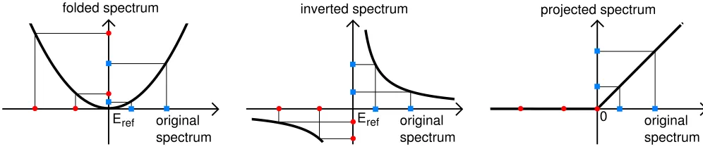
a. Folded spectrum The folded spectrum method in-volves folding the energy spectrum of a matrixHaround a reference energyEref, where the spectrum ofHis found from the eigenvalue equation Hx=ǫx. This leads to a new eigenvalue equation which the eigensolutions of the original equation also satisfy:
(H−ErefI)2x= (ǫ−Eref)2x. (3)
The smallest eigenvalues of this new matrix are related to those of H nearestEref, so that by setting Eref to a value near the center of the energy range covered by the conduction states, they can be found by solving the new eigenvalue equation. It can also be generalized to account for the use of a non-orthogonal basis set39, giving the following:
(H−ErefS)S−1(H−ErefS)x= (ǫ−Eref)2Sx. (4)
This is illustrated by Fig. 1, which contains a schematic showing the effect of the folded spectrum method on a set of example eigenvalues. This method has been used pre-viously for example to study the conduction band min-imum for silicon within the tight-binding method40, as well as in studies of quantum dots41,42.
b. Shift invert Shift invert is another method of spectral transformation which can be used to find ex-tremal eigenvalues. Starting from a given generalized eigenvalue equation Hx = ǫSx, the Hamiltonian is shifted with respect to some reference energy and then inverted, giving:
(H−ErefS)−1Sx= (ǫ−Eref)−1x. (5)
However, even if both S and H are Hermitian, (H−ErefS)−1S will not generally be Hermitian43,44, which could result in decreased numerical efficiency. The most straightforward method of ensuring that the trans-formed Hamiltonian is Hermitian is to pre-multiply by the overlap matrix, giving:
S(H−ErefS)−1Sx= (ǫ−Eref)−1Sx. (6)
For this case, the eigenvalues of the original matrix will be calculated in descending order, starting from the refer-ence energy, as demonstrated in Fig. 1, which contains a diagram showing the transformation of a set of example eigenvalues following the application of shift invert. In
order to correctly calculate the conduction states, the ref-erence energy should therefore be set between the high-est required conduction band and the state immediately above (shift invert variant +). One way to avoid this problem is to multiply the new Hamiltonian by minus one, reversing the order of calculation and therefore al-lowing the conduction states to be calculated in ascend-ing order startascend-ing from the LUMO (lowest unoccupied molecular orbital), simply by setting the reference energy to be just above the HOMO (highest occupied molecular orbital) (shift invert variant -).
The shift invert method can suffer from stability prob-lems, which can be reduced by adding an imaginary com-ponent, iµ, to the reference energy, however this means that the Hamiltonian once again loses its Hermiticity, cre-ating the possibility of imaginary eigenvalues. This can be avoided by combining two shift invert transformations, such that a small positive imaginary component is added to the reference energy for the first transformation and a negative component is added to the second, thereby eliminating all imaginary components. This gives the fi-nal generalized eigenvalue equation:
S
HS−1H−2ErefH+ Eref2 +µ2
S−1
Sx (7)
= (ǫ−Eref)−2x.
In this case the eigenvalues appear in an unfavourable or-der, such that as the transformed eigenvalues increase in energy,|ǫ−Eref|decreases , i.e. the eigenvalues furthest from Eref will be found first. Multiplying the Hamilto-nian by minus one will reverse the order, returning to the situation where eigenvalues closest to the reference energy are found first (shift invert variant i). This resem-bles the folded spectrum method in that the conduction and valence states again become mixed, and so a careful choice of reference energy is needed.
c. Projection The density operator is defined ac-cording to Eq. (1), where thefn are the occupation
num-bers which are assumed to be 1 for valence states and 0 for conduction states within the test program. The den-sity operator ˆρis a projection operator onto the subspace of states occupied by the valence states, so that project-ing ˆρonto ˆHand solving the new eigenvalue equation will give only the valence eigenstates. Alternatively, project-ing with 1−ρˆ, where the 1 is defined in the psinc basis, will leave only contributions from the conduction states. This is illustrated in Fig. 1, which contains a schematic demonstrating the effect of projecting the Hamiltonian in this manner on a set of example eigenvalues.
One problem which can arise due to the imposition of localization constraints during a calculation is that
ˆ
H and ˆρmay not commute exactly, which will result in the projected Hamiltonian no longer being Hermitian. This can be overcome by projecting twice, so that the expression
ˆ
H−ρˆHˆρˆ (8)
folded spectrum inverted spectrum projected spectrum
original spectrum Eref
original spectrum
Eref original
spectrum 0
FIG. 1. (Color online) Schematics comparing the three methods for the calculation of unoccupied states. The original spectrum is shown on thex-axis and the transformed spectrum on they-axis, with thick black curves depicting the relationship between the two sets of eigenvalues. The occupied states are shown as (red) circles and the unoccupied states as (blue) squares, with the reference energy arbitrarily chosen to be in the gap for the folded spectrum and shift invert methods.
energy spectrum where all the valence energies are equal to zero, which is only desirable when all the conduction energies are negative and so more favourable in energy than the zeroed valence states. To avoid this problem the energy spectrum is shifted so that all the valence states become higher in energy than the conduction states. This shift must be greater than or equal to the highest con-duction energy, the value of which can be easily found using conjugate gradients, as only the highest energy is required. The projected Hamiltonian can be modified to include the shift,σ, so that the final operator is:
ˆ
H−ρˆHˆ −σρ.ˆ (9)
In practice, the shiftσis set to be higher than the highest conduction energy, so that in general it remains constant even when there are changes in the highest eigenvalue, adding stability to the minimization process. If neces-sary, it can also be updated during the calculation.
C. Results and discussion
These five methods were tested and compared for a sys-tem with a Kronig-Penney potential45using the block up-date preconditioned conjugate gradients method24. By applying the appropriate level of preconditioning and se-lecting a good choice of reference energies, the results in Table I were obtained. No shift was applied for the pro-jection method. In attempting to choose good values for the reference energies, it was verified that a poor choice can result in significantly slower convergence. For all of the methods the total conduction energies calculated were accurate to within 10−10 Ha of the correct result.
The results show that the different methods are fairly similar in terms of both speed and accuracy, with the projection method as the clear favorite. An important requirement of the selected method is the need for linear-scaling. Whilst this is hard to test within this basic im-plementation due to the lack of localization and sparse matrix multiplication, it can be shown that with the ap-propriate level of preconditioning, the number of
itera-TABLE I. Results for the different conduction methods, show-ing averages for time taken and the number of iterations for a total of 100 calculations with randomly generated starting guesses for the eigenvectors. Shift invert +, - and i refer to the three variants of the shift invert method discussed in the text. The first form of the projection method was applied, without the use of a shift.
Method Avg. time Avg. number
taken (s) of iterations
Folded spectrum 2.39 182
Shift invert + 2.34 158
Shift invert - 2.23 170
Shift invert i 5.48 463
Projection 1.21 36
tions required for increasing system size remains approx-imately constant for the projection method. Combined with the fact that the method mainly consists of ma-trix multiplications, it seems likely that favorable scaling could be achieved when implemented within local-orbital methods.
The reason for the relatively large number of iterations required for the folded spectrum method can be seen by considering the condition number, which will be higher for the folded Hamiltonian. Using the approximate ex-pression21:
κ≈ (ǫmax−ǫmin) ǫgap
, (10)
it is clear that the largest eigenvalueǫmax will be much bigger for the transformed Hamiltonian, and thus so will the condition number, κ. Therefore when using an it-erative minimization scheme, convergence will be slower compared to solving the original equation.
[image:5.595.57.555.51.157.2] [image:5.595.318.562.327.419.2]states will need to be calculated in order to get the low-est conduction states. Additionally a poor choice of ref-erence energy will result in slower convergence for the shift invert method. For example, if the reference energy is too close to a given eigenvalue, such that the differ-ence between Eref and ǫ is very small compared to the distance to other eigenvalues, the magnitude of the eigen-value for the new system will be much greater than all other eigenvalues. This will result in a high condition number, so care must be taken to find a good reference energy. The projection method, however, has the advan-tage that no reference energy is required and therefore it is more automatic. Additionally, the density matrix is already calculated within a local-orbital calculation and so can easily be reused.
For the case of all three methods, the accuracy of the conduction states will clearly be affected by the accuracy with which the potential has been calculated. However, the projection method will also be affected by the accu-racy of the valence density matrix, whereas the folded spectrum and shift invert methods will not. This will be particularly significant when the localization and trunca-tion approximatrunca-tions required for linear-scaling behaviour are applied.
D. Implementation in ONETEP
The methods outlined above were applied directly to the solution of an eigenvalue equation. However in a real
onetepcalculation, the system is solved using a density
matrix scheme, within the representation of a basis of NGWFs. It is therefore necessary to adapt the methods described above for use within this context. As the pro-jection method has proven to be the most favorable, this is the one which was subsequently focussed on.
Two sets of NGWFs are now required, {|φαi} for the
valence states, and{|χαi}for the conduction states. The
ground stateonetepcalculation already provides access to the valence density matrix ρ and kernel K, overlap
matrix Sφ and Hamiltonian Hφ. The additional
con-duction matrices will be labelled as follows: Sχ is the
conduction overlap matrix, T is the valence-conduction cross overlap matrix defined as Tαβ = hφα|χβi, Hχ is
the (unprojected) conduction Hamiltonian, Hprojχ is the projected conduction Hamiltonian, Q is the conduction density matrix andM is the conduction density kernel. These are all represented by atom-blocked sparse matri-ces10,46, such that all matrix-matrix operations are possi-ble in asymptotically linear-scaling computational effort, due to the strict truncation.
The final expression for the projected conduction Hamiltonian, including the shift, σ, is therefore defined
as follows:
Hχproj
αβ=hχα|Hˆ −ρˆ
ˆ
H−σρ|χˆ βi (11)
= (Hχ)αβ− T†KHφKTαβ
+σ T†KSφKT
αβ
The energy expressionE= tr
MHproj
χ
can then be min-imized by optimizing both the set of conduction NGWFs and the conduction kernel. Extra terms will be needed in the NGWF gradient, but otherwise this follows the same procedure as a standardonetepcalculation, with-out the need for self-consistency. Once the set of conduc-tion NGWFs has been optimized, the Hamiltonian can be diagonalized in a joint basis of valence and conduction NGWFs to give an improved eigenvalue spectrum. This allows eigenvalues and other properties to be calculated in a basis that is capable of representing both the valence and conduction states of the system.
E. Calculating optical spectra
As stated in the introduction, the calculation of ex-perimental spectra in general and optical spectra in par-ticular can be highly useful both in predicting and un-derstanding experimental results and can be applied to a diverse range of problems. The method followed for the calculation of optical absorption spectra is that47applied
incastep48, a cubic-scaling plane-wave pseudopotential
(PWPP) DFT code which can use the same pseudopoten-tials asonetep, and so is ideal for comparison of results. The method employed is described briefly below.
Starting from time-dependent perturbation theory, one can derive Fermi’s golden rule, an expression giving the probability of a particular electronic transition. It in-volves a joint density of states between valence and con-duction states, which is weighted by optical matrix el-ements. Matrix elements with a value of zero indicate that a given transition is forbidden, whereas nonzero ma-trix elements define the strength of the transition. These matrix elements take the form of a complex exponential, which in the long-wavelength limit can be related to po-sition matrix elements using the dipole approximation, where the exponential is expanded in a Taylor series and terms above first order are neglected. In this manner, the imaginary part of the dielectric function can be written as:
ε2(ω) = 2e2π
Ωε0 X
k,v,c
|hψc
k|ˆq·r|ψkvi|
2
δ(Ekc−Ekv−~ω),
(12) wherev andc denote valence and conduction bands re-spectively,|ψn
kiis the nth eigenstate at a given k-point
with a corresponding energy En
k, Ω is the cell volume, ˆ
q is the direction of polarization of the photon and~ω
onetep calculations, it is assumed that a large enough supercell will be used such that only the gamma point need be considered. As the system size increases, this will become an increasingly exact approximation, so that the accuracy of the density of states will improve for bigger systems. This could be extended in future using methods for interpolating band structures inonetepthat will be published elsewhere. For the purposes of this work, how-ever, all calculations have been restricted to the gamma point only. From the imaginary part of the dielectric function one can then also calculate the real part using the appropriate Kramers-Kronig relation.
In bothonetep and castep periodic boundary con-ditions are used, in which the position operator is known to be undefined. Due to the strict localization of the NGWFs in onetep, it is possible to calculate position matrix elements between eigenstates for molecules, pro-viding the NGWF radii are sufficiently small such that no NGWFs associated with the molecule overlap with any NGWFs associated with its periodic image. How-ever for periodic systems it becomes necessary to use the momentum operator. Momentum matrix elements can be easily related to position matrix elements by consid-ering the commutator with the Hamiltonian, but when non-local pseudopotentials are being used, one must be careful to include the commutator between the position operator and the non-local potential. The relation is thus written49:
hφf|r|φii=
1
iωmhφf|p|φii+
1
~ωhφf|
h ˆ
Vnl,r i
|φii. (13)
In practice, the commutator term is calculated using the following identity50:
(∇k+∇k′)
Z
e−ik·rVnl(r,r′)eik
′·r′
drdr′
(14)
=i
Z
e−ik·r[Vnl(r,r′)r′−rVnl(r,r′)]eik
′·r′
drdr′,
where the derivative can either be calculated directly or using finite differences in reciprocal space. The matrix elements are thus calculated in this manner and used to form a weighted density of states, which is smeared using Gaussian functions.
[image:7.595.317.566.50.170.2]For the purposes of comparison with experiment, it is sometimes desirable to make use of the scissor oper-ator, whereby the conduction band energies are rigidly shifted upwards such that the DFT Kohn-Sham band gap is equal to experimental values. Whilst this is not anab initio correction, in practice relatively good agree-ment can be found with experiagree-ment in this manner for many systems without the need for more computation-ally intensive methods, such as theGW approximation, although there will be a number of occasions when it becomes necessary to use less approximate methods.
FIG. 2. Schematics showing the structures of thetrans (left) andcis(right) isomers of metal-free phthalocyanine. C atoms are shown in white, N atoms in gray and H atoms in black.
III. RESULTS AND DISCUSSION
A. Metal-free phthalocyanine
As stated in section II A, onetep is particularly effi-cient at treating molecules, and so metal-free phthalo-cyanine was chosen as a good test system on which to apply the conduction state method. As it contains only 58 atoms, calculations could also be performed using castep, which has been used for all the tradi-tional PWPP DFT results given. Corresponding plane-wave/psinc kinetic energy cut-offs and identical norm-conserving pseudopotentials were used for both codes. In all calculations the local-density approximation (LDA) exchange-correlation functional was used. Phthalocya-nines and their derivatives are commonly used as dyes and are also of interest in a number of other fields, in-cluding use in photovoltaic cells51 and molecular spin-tronics52and so metal-free phthalocyanine also provides an interesting test case for the calculation of optical ab-sorption spectra.
The atomic coordinates for metal-free phthalocyanine were taken from neutron diffraction data53with C2
h
sym-metry and the inner H atoms attached to opposite N atoms. Additional symmetry constraints were then ap-plied by averaging the atomic positions to give the higher symmetry D2hwith the inner H atoms attached to both
opposite and adjacent N atoms (trans andcis forms re-spectively), and finally a geometry optimized structure was calculated using traditional DFT, which also has a trans-D2h symmetry but differs in bond lengths from
the other D2h structure. Diagrams of the trans and cis
forms are shown in Fig. 2. Table II shows the ground state energies for each structure relative to the geometry optimized result, with the higher symmetry structures lower in energy. Very good agreement is achieved be-tween the onetep and traditional DFT results. Both
theonetep and PWPP calculations were performed at
TABLE II. Comparison betweenonetepand PWPP
ground-state total energies for four different structures of metal-free phthalocyanine, relative to the lowest energy geometry opti-mized structure. The energy difference between theonetep
and PWPP results for the geometry optimized structure is 0.163 eV.
Structure E−Egeom / eV
onetep PWPP
C2h 1.554 1.553
cis-D2h 1.875 1.874
trans-D2h 0.952 0.951
30 20 10 0 10 20 30
-10 -5 0 5 10
DOS
Energy / eV
PWPP ONETEP ONETEP+cond
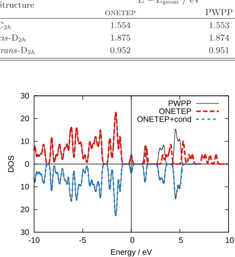
FIG. 3. (Color online) Density of states comparing results fromonetepwith PWPP results for the geometry-optimized
structure of metal-free phthalocyanine, plotted with a Gaus-sian smearing width of 0.1 eV, using conduction NGWF radii of 16 Bohr. The DOS is truncated after the first 16 conduc-tion states, and theonetep+cond curve shown is calculated
in the joint valence-conduction NGWF basis.
Sixteen conduction states were optimized, with four con-duction NGWFs for each atomic species, and a radius of 16 Bohr was used for the density of states (DOS) calcu-lations, whilst 13 Bohr was sufficient to achieve almost perfect agreement with traditional DFT for the optical absorption spectra. This difference in NGWF radii re-quired for good convergence of DOS and optical absorp-tion spectra is discussed in secabsorp-tion III C. The DOS for the geometry optimized structure is shown in Fig. 3, which comparesonetepresults both with and without conduc-tion NGWFs to those found using the PWPP method. Without the conduction NGWFs, theonetepresults dif-fer greatly from the PWPP results, but with the addi-tion of conducaddi-tion NGWFs, excellent agreement with the PWPP method is achieved. A state-by-state comparison confirmed the existence of a one-to-one correspondence between theonetepandcastepconduction eigenstates. Optical absorption spectra were then calculated using
2 2.5 3 3.5 4
ε2
Energy / eV Q
cis-D2h
C2h
trans-D2h
geom
exp
FIG. 4. (Color online) The imaginary component of the di-electric function calculated in onetep and plotted for four
different structures of metal-free phthalocyanine as indicated on the graph (‘geom’ refers to the geometry optimized struc-ture). Results from the PWPP method are indistinguishable and so not plotted. A Gaussian smearing width of 0.01 eV is used, with conduction NGWF radii of 13 Bohr and a scissor operator of 0.4 eV. Experimental results in solution (labelled ‘exp’) are also included with the peaks shown as vertical lines for clarity and the calculated results vertically scaled arbi-trarily for easier comparison. The position of the Q-bands is indicated below the x-axis.
both the position operator and the momentum operator (including the non-local commutator) for all four struc-tures, and in all cases the two methods agreed almost perfectly with the PWPP results for the energy range considered. The addition of a greater number of conduc-tion states is unnecessary for this energy range, confirm-ing that the calculation of unbound conduction states will not always be needed.
It should be emphasized here that the aim of this work is calculate absorption spectra within DFT and so find good agreement with conventional DFT implemen-tations, rather than go beyond DFT and achieve good agreement with experiment. However, useful insight can be achieved through comparision with experiment, and so the absorption spectra for the four structures were compared with experimental results in solution51, apply-ing a scissor operator of 0.4 eV, and arbitrarily scalapply-ing the height of the imaginary part of the dielectric function to facilitate easier comparison with experiment, as shown in Fig. 4. The spectra are indeed distinguishable, despite the very small differences in the atomic structures.
[image:8.595.59.299.135.398.2]lower symmetry of the metal-free phthalocyanine struc-ture as compared to metal phthalocyanines is the cause for this Q-band splitting, which is not observed for metal phthalocyanines. This agrees with the observation that the higher symmetrytrans-D2hstructure exhibits a lower
degree of splitting than thetrans-C2h structure. The
Q-band splitting for the geometry optimized structure is 0.02 eV, which is significantly less than the experimental value of 0.09 eV, implying that the LDA is not sufficiently accurate to calculate the correct structure.
There have already been a number of studies54–57 of the electronic structure and absorption spectra of metal-free phthalocyanine, with which the above results are consistent, confirming that this is a useful system to demonstrate the ability of theoretical optical absorption spectra as implemented here to distinguish between sim-ilar geometries.
B. Poly(para-phenylene)
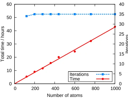
Conjugated polymers such as poly(para-phenylene) have a wide range of applications due to their electrolu-minescent properties, including LEDs and solar cells58–60 and so this also provides an interesting system to study as a test case for the calculation of optical absorption spectra. As a periodic system, it is also ideal for test-ing the scaltest-ing of the projection method, by increastest-ing the size of the unit cell and comparing the time taken to calculate the conduction states. The structure for two unit cells was obtained by performing a geometry optimization with a PWPP code using the structure of Ambrosch-Draxlet al.61as a starting guess, with the final structure shown in Fig. 5. A cut-off energy of 1115 eV was found to be necessary for good convergence of the results. All calculations were performed at the Gamma point only, with nok-point sampling, to allow for direct comparison between the two codes. Ground state cal-culations were first performed with one NGWF per H atom and four NGWFs per C atom and a fixed radius of 10 Bohr. Conduction calculations were then performed using four NGWFs for all atomic species with a fixed radius of 14 Bohr. The number of conduction states cal-culated was set to include all negative eigenvalues for the smallest system (corresponding to two unit cells of PPP) and increased linearly with system size. Fig. 6 shows the scaling behavior of onetep for the conduction calcula-tion. Neither the valence nor conduction density kernels were truncated, however, the behaviour of onetep is shown to be approximately linear up to 1000 atoms, and it is expected that this trend will continue up to larger system sizes.
[image:9.595.320.559.53.131.2]The density of states was plotted for varying chain lengths of PPP, with the graph for 120 atoms shown in Fig. 7. As with metal-free phthalocyanine, excellent agreement with the PWPP results is achieved for the conduction calculation. The imaginary component of the dielectric function was also calculated for varying chain
FIG. 5. Schematic showing the structure of a unit of poly(para-phenylene) from two directions. C atoms are shown in white and H atoms in black.
0 10 20 30 40 50 60
0 200 400 600 800 1000
0 5 10 15 20 25 30 35 40
Total time / hours
Iterations
Number of atoms Iterations Time
FIG. 6. (Color online) Graph showing the scaling ofonetep
conduction calculations for increasing chain lengths of PPP. Calculations were performed on 8 nodes and therefore a total of 32 cores. The total time taken foronetepis approximately
linear up to 1000 atoms and the number of NGWF iterations required for convergence shown in the inset is shown to be constant with an increasing number of atoms.
lengths, using the momentum operator formulation. The result for 120 atoms is shown in Fig. 8. Again, nearly perfect agreement with the PWPP method was achieved with the conduction NGWF basis, whereas the valence NGWF basis only calculation showed big discrepancies not only in the positions of the peaks, but also in the relative strengths.
C. Limitations of the method
The projection method has proven to be a good method of optimizing a set of NGWFs that are capable of representing the conduction states to a good degree of accuracy. However, there are some limitations to the method, which will be discussed below.
[image:9.595.329.553.209.381.2]60 40 20 0 20 40 60
-10 -5 0 5 10
DOS
Energy/eV
[image:10.595.327.556.64.236.2]PWPP ONETEP ONETEP+cond
FIG. 7. (Color online) Density of states calculated using
onetepand a PWPP code for 120 atoms of PPP with
con-duction NGWF radii of 14 Bohr and a Gaussian smearing width of 0.1 eV. The onetep+cond curve is from the joint
valence-conduction NGWF basis, and has been plotted so that only those conduction states which have been optimized are included. The same number of states have been plotted for both theonetepand PWPP curves.
20 15 10 5 0 5 10 15 20
2 3 4 5 6 7 8 9
ε2
Energy / eV
PWPP ONETEP ONETEP+cond
FIG. 8. (Color online) The imaginary component of the di-electric function calculated using a traditional PWPP code andonetepboth with and without a conduction calculation
for 120 atoms of PPP. Conduction NGWF radii of 14 Bohr and a Gaussian smearing width of 0.2 eV are used.
With increasing NGWF radii the eigenvalues tend to-wards the correct Kohn-Sham eigenvalues, however when one uses such large radii the prefactor of the calcula-tion becomes dominant, so that even though the over-all behaviour is still linear-scaling, the crossover point at which the method becomes quicker than cubic-scaling codes will occur at systems with a greater number of
-7 -6.5 -6 -5.5 -5
20 40 60 80 100
-7 -6 -5 -4 -3 -2
log
10
(RMS gradient)
log
10
(E-E
final
)
Iteration RMS gradient
Energy
FIG. 9. (Color online) Demonstration of the appearance of a local minimum, where the RMS gradient increases for a period whilst the energy continues to decrease. This was for the geometry-optimized structure of metal-free phthalocyanine at a radius of 18 Bohr with four extra states being optimized.
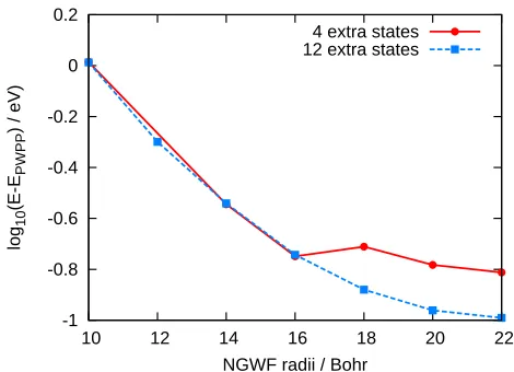
atoms. However, for applications considered here, no-tably the calculation of optical absorption spectra, often only lower energy bound states are required, as many of the interesting features in optical spectra are transitions between bands close to the gap and one is interested in a relatively low energy range. Therefore in practice this limitation on the method is less serious than it first ap-pears to be. Additionally, it has been observed that the lower energy conduction states converge with respect to NGWF radius faster than those with higher energy, and so if the lower energy bound states only are considered, it no longer becomes necessary to use such large NGWF radii to achieve a good level of convergence in the optical absorption spectra. It was for this reason that smaller conduction NGWF radii were used for the absorption spectra compared to the DOS of metal-free phthalocya-nine, as presented in section III A.
[image:10.595.70.297.67.236.2] [image:10.595.69.297.374.543.2]-1 -0.8 -0.6 -0.4 -0.2 0 0.2
10 12 14 16 18 20 22
log
10
(E-E
PWPP
) / eV)
NGWF radii / Bohr 4 extra states 12 extra states
FIG. 10. (Color online) Comparison of conduction energy convergence with respect to conduction NGWF radii for dif-ferent numbers of extra states, for the geometry-optimized structure of metal-free phthalocyanine. The energy difference is calculated with respect to the traditional PWPP result. A discontinuity appears in the curve at 18 Bohr when four ad-ditional states are optimized, demonstrating problems with local minima, whilst optimizing 12 additional states is suffi-cient to overcome the problem.
[image:11.595.63.298.66.236.2]then reducing the number of states to that actually re-quired, regenerating the conduction density kernel and proceeding with the calculation. This first stage aims to overcome the problem of poor initial ordering of states, whilst the second stage will allow for closer optimization of those states actually required. This is illustrated by Table III, where the LUMO+14 state is initially much higher in energy and so if no additional states are in-cluded the NGWFs are not optimized to represent it, so that it ends up significantly higher in energy than other states. If, however, four additional states are included, this is sufficient to reorder the states and it becomes lower in energy.
TABLE III. Initial energies and values after 5 iterations both with and without optimizing extra states for three different eigenstates of the geometry-optimized structure of metal-free phthalocyanine with conduction NGWF radii of 14 Bohr. States shown in bold are those which are among the 16 low-est states, and thus being included in the conduction NGWF optimization. Without the optimization of extra states, the LUMO+14 state is not optimized and so remains high in en-ergy, whilst with the addition of four extra states, the correct order is found and the LUMO+14 is significantly lowered in energy.
State Initial 0 extra states 4 extra states
LUMO+14 0.628 >0.368 -0.042
LUMO+15 0.355 0.045 0.039
LUMO+16 0.259 0.082 0.061
As well as the above-mentioned problems, there are a number of parameters which require more careful con-sideration when selecting appropriate values than in a ground stateonetepcalculation, where they can be set automatically. This includes the number of conduction states one is trying to represent, the number of NG-WFs one chooses for each atom, the number of additional states to be optimized and the number of iterations for which these extra states are optimized. Some of these parameters, such as the number of iterations to perform in the first stage of the local minima avoiding scheme, have less of an effect on the final result, but for many of these parameters, the effect of different values appears to be strongly system-dependent. One must therefore per-form careful convergence tests to ensure that the result-ing states do not correspond to any local minima. This will require variation of the number of NGWFs per atom, convergence with respect to NGWF radii, and an increase in the number of extra conduction states requested, un-til consistent results are achieved, with a smooth curve of energy against NGWF radii, and sensible convergence of the NGWFs during a calculation. By following these strategies one can become confident that accurate results have been achieved.
It should also be noted that the iterative energy min-imization scheme used here requires the presence of a band gap, which for the conduction calculation trans-lates as a gap between the highest optimized conduction state, and the lowest unoptimized conduction state. As one approaches the continuum of conduction states, this gap will become increasingly small, which could result in poor convergence behaviour.
Finally, it is observed that whilst problems have been encountered with the projection method, a clear strat-egy has been outlined both for identifying and resolving them.
IV. CONCLUSIONS
[image:11.595.54.298.662.721.2]peak and compare spectra from very similar atomic struc-tures has been demonstrated, through the application to both a molecular and an extended system. Furthermore, it also forms the basis of future extensions both to more accurate methods of calculating optical spectra, and to calculating other types of spectra, such as electron en-ergy loss spectra and x-ray absorption and photoemission spectra.
ACKNOWLEDGMENTS
This work was supported by the UK Engineering and Physical Sciences Research Council (EPSRC).
Calcula-tions were performed on CX1 (Imperial College London High Performance Computing Service). N.D.M.H. ac-knowledges the support of the Engineering and Phys-ical Sciences Research Council (EPSRC Grant No. EP/G055882/1) for postdoctoral funding through the HPC Software Development call 2008/2009. P.D.H. ac-knowledges support from the Royal Society in the form of a University Research Fellowship.
∗ E-mail: [email protected]
1 P. Hohenberg and W. Kohn, Phys. Rev.136, B864 (1964). 2 W. Kohn and L. J. Sham, Phys. Rev.140, A1133 (1965). 3 G. Galli and M. Parrinello, Phys. Rev. Lett. 69, 3547
(1992).
4 P. Ordej´on, D. A. Drabold, R. M. Martin, and M. P. Grumbach, Phys. Rev. B51, 1456 (1995).
5 E. Hern´andez and M. J. Gillan, Phys. Rev. B 51, 10157 (1995).
6 J.-L. Fattebert and J. Bernholc, Phys. Rev. B 62, 1713 (2000).
7 C.-K. Skylaris, A. A. Mostofi, P. D. Haynes, O. Di´eguez, and M. C. Payne, Phys. Rev. B66, 035119 (2002). 8 C.-K. Skylaris, P. D. Haynes, A. A. Mostofi, and M. C.
Payne, J. Chem. Phys.122, 084119 (2005).
9 P. D. Haynes, C.-K. Skylaris, A. A. Mostofi, and M. C. Payne, Phys. Status Solidi B243, 2489 (2006).
10 N. D. M. Hine, P. D. Haynes, A. A. Mostofi, C.-K. Sky-laris, and M. C. Payne, Comput. Phys. Commun. 180, 1041 (2009).
11 N. D. M. Hine, M. Robinson, P. D. Haynes, C.-K. Skylaris, M. C. Payne, and A. A. Mostofi, Phys. Rev. B83, 195102 (2011).
12 R. W. Godby, M. Schl¨uter, and L. J. Sham, Phys. Rev. Lett.56, 2415 (1986).
13 F. Gygi and A. Baldereschi, Phys. Rev. Lett. 62, 2160 (1989).
14 L. Hedin, Phys. Rev.139, A796 (1965).
15 R. W. Godby and R. J. Needs, Physica ScriptaT31, 227 (1990).
16 R. Del Sole, L. Reining, and R. W. Godby, Phys. Rev. B
49, 8024 (1994).
17 W. Kohn, Phys. Rev. Lett.76, 3168 (1996).
18 S. Ismail-Beigi and T. A. Arias, Phys. Rev. Lett.82, 2127 (1999).
19 W. Kohn, Int. J. Quantum Chem.56, 229 (1995). 20 L. He and D. Vanderbilt, Phys. Rev. Lett.86, 5341 (2001). 21 S. Goedecker, Rev. Mod. Phys.71, 1085 (1999).
22 G. Galli, Curr. Opin. Solid State Mater. Sci.1, 864 (1996). 23 D. R. Bowler, T. Miyazaki, and M. J. Gillan, J. Phys.:
Condens. Matter14, 2781 (2002).
24 A. A. Mostofi, P. D. Haynes, C.-K. Skylaris, and M. C. Payne, J. Chem. Phys.119, 8842 (2003).
25 P. Haynes, C.-K. Skylaris, A. Mostofi, and M. Payne,
Chem. Phys. Lett.422, 345 (2006).
26 R. McWeeny, Rev. Mod. Phys.32, 335 (1960).
27 E. Hern´andez and M. J. Gillan, Phys. Rev. B51, 10157 (1995).
28 P. D. Haynes and M. C. Payne, Phys. Rev. B 59, 12173 (1999).
29 C.-K. Skylaris and P. D. Haynes, J. Chem. Phys. 127, 164712 (2007).
30 C.-K. Skylaris, P. D. Haynes, A. A. Mostofi, and M. C. Payne, J. Phys.: Condens. Matter17, 5757 (2005). 31 J. A. Berger, L. Reining, and F. Sottile, Phys. Rev. B82,
041103 (2010).
32 P. Umari, G. Stenuit, and S. Baroni, Phys. Rev. B 81, 115104 (2010).
33 F. Giustino, M. L. Cohen, and S. G. Louie, Phys. Rev. B
81, 115105 (2010).
34 D. Rocca, D. Lu, and G. Galli, J. Chem. Phys.133, 164109 (2010).
35 J. K. L. MacDonald, Phys. Rev.46, 828 (1934).
36 L.-W. Wang and A. Zunger, J. Chem. Phys. 100, 2394 (1994).
37 T. Ericsson and A. Ruhe, Math. Comp.35, 1251 (1980). 38 E. Hern´andez, M. J. Gillan, and C. M. Goringe, Phys.
Rev. B55, 13485 (1997).
39 A. R. Tackett and M. Di Ventra, Phys. Rev. B66, 245104 (2002).
40 A. S. Martins, T. B. Boykin, G. Klimeck, and B. Koiller, Phys. Rev. B72, 193204 (2005).
41 H. Fu and A. Zunger, Phys. Rev. B56, 1496 (1997). 42 A. Franceschetti and A. Zunger, Phys. Rev. Lett.78, 915
(1997).
43 P. D. Cha and W. Gu, J. Sound Vib.227, 1122 (1999). 44 G. W. Stewart, Matrix Algorithms Volume 2:
Eigensys-tems (Siam, 2001).
45 C. Kittel,Introduction to Solid State Physics, 7th ed. (John Wiley and Sons, 1996).
46 N. D. M. Hine, P. D. Haynes, A. A. Mostofi, and M. C. Payne, J. Chem. Phys.133, 114111 (2010).
47 C. J. Pickard, Ab initio Electron Energy Loss Spec-troscopy, Ph.D. thesis, University of Cambridge (1997). 48 S. J. Clark, M. D. Segall, C. J. Pickard, P. J. Hasnip, M. J.
Probert, K. Refson, and M. C. Payne, Z. Kristallogr.220, 567 (2005).
50 C. Motta, M. Giantomassi, M. Cazzaniga, K. Gal-Nagy, and X. Gonze, Comput. Mater. Sci.50, 698 (2010). 51 N. Kobayashi, S.-i. Nakajima, H. Ogata, and T. Fukuda,
Chem. Eur. J.10, 6294 (2004).
52 X. Shen, L. Sun, E. Benassi, Z. Shen, X. Zhao, S. Sanvito, and S. Hou, J. Chem. Phys.132, 054703 (2010).
53 B. F. Hoskins, S. A. Mason, and J. C. B. White, J. Chem. Soc. D , 554b (1969).
54 R. Fukuda, M. Ehara, and H. Nakatsuji, J. Chem. Phys.
133(2010).
55 X. D. Gong, H. M. Xiao, and H. Tian, Int. J. Quantum Chem.86, 531 (2002).
56 H. Cortina, M. L. Senent, and Y. G. Smeyers, J. Phys. Chem. A107, 8968 (2003).
57 P. N. Day, Z. Wang, and R. Pachter, J. Mol. Struct.: THEOCHEM455, 33 (1998).
58 A. Moliton and R. C. Hiorns, Polym. Int.53, 1397 (2004). 59 P. Lane, M. Liess, Z. Vardeny, M. Hamaguchi, M. Ozaki,
and K. Yoshino, Synth. Met.84, 641 (1997).
60 J. H. Burroughes, D. D. C. Bradley, A. R. Brown, R. N. Marks, K. Mackay, R. H. Friend, P. L. Burns, and A. B. Holmes, Nature347, 539 (1990).