GPU implementation of partial order reduction

(1)

GPU IMPLEMENTATION

OF PARTIAL-ORDER

REDUCTION

MASTER THESIS

Thomas Neele

Faculty of Electrical Engineering, Mathematics

and Computer Science (EEMCS)

Formal Methods and Tools

Exam committee:

(2)

Abstract

Model checking using GPUs has seen increased popularity over the last years. Be-cause GPUs have only a limited amount of memory, only small to medium-sized systems can be verified. We improve memory efficiency for explicit-state GPU model checking by applying on-the-fly partial-order reduction. The correctness of the pro-posed algorithms is proved using a new version of the cycle proviso. Benchmarks show that our implementation achieves a reduction similar to or better than the state-of-the-art techniques for CPUs, while the runtime overhead is acceptable.

(3)

Chapter 1 Introduction

This chapter gives an introduction by providing a short overview of the field of model checking and general-purpose GPU programming. Then, it defines the contributions of this thesis and discusses related work. Finally, it gives an overview of the structure of this thesis.

1.1 Overview

In the research field of formal methods, model checking [2, 14] is a popular technique for proving the correctness of concurrent systems. However, the practical applica-bility is still limited by the problem of state-space explosion. This is due to the many possible interleavings of actions of concurrent processes and the many con-figurations of the state vector describing the process variables. In the early days, model checkers relied on the newest hardware to improve their performance. In recent years, however, sequential performance has not seen major improvements. A speed up can now only be gained by implementing parallel algorithms. While distributed systems saw a lot of popularity in the early 2000s, the focus has since shifted to the multi-core shared-memory architecture that is used in all modern-day hardware. Designing multi-threaded algorithms for this hardware brings forward new challenges: to achieve good scalability, resource contention between the threads should be kept to a minimum. Furthermore, subtle errors in the implementation may break the correctness. Most of the popular model checkers already have multi-core implementations [5, 13, 16, 23, 27].

(6)

is called general-purpose GPU (GPGPU) programming. Since the introduction of NVIDIA’s CUDA [1] (a complete API for GPGPU programming) in 2008, GPUs have been used in many different applications, including model checking [4, 19, 44, 41].

Although GPUs do not seem suited to aid model checking due to their limited amount of memory, the massive number of threads that run in parallel makes GPUs attractive for this computationally intensive task. Their parallel power can speed-up state-space exploration by up to two orders of magnitude [3, 18, 41, 44]. Moreover, the amount of memory available on GPUs has increased significantly over the last years. Therefore, it is interesting to investigate the potential of GPUs, at least for future interest. Research has shown that, although GPUs can greatly outperform CPUs, they quickly run out of memory for larger models [7]. Therefore, the practical applicability of GPU model checking is still limited.

An approach to increase the memory efficiency of explicit-state model checking is by applying reduction techniques. Several approaches have been proposed, among others: partial-order reduction (POR) [38, 37, 22], symmetry reduction [25] and bisimulation minimisation [35]. All of these techniques exploit the fact that the state space may contain several states that are similar with respect to the property under consideration. By merging or not exploring the similar states, the memory footprint of the state-space exploration is reduced. When done efficiently, the amount of time required to check the property under consideration can also be reduced. Partial-order reduction and symmetry reduction can be performed on-the-fly, i.e. while exploring the state-space. Bisimulation minimisation can only be applied after the whole state space has been generated.

Contributions Our contributions are as follows:

1. We improve the memory efficiency of GPU model checking. To that end, we extend GPUexplore [41, 42], one of the first tools that runs a complete model checking algorithm on the GPU, with POR. We propose GPU algorithms for three practical approaches to POR, based on ample [24], cample [9] and stubborn sets [38].

2. We improve the cample-set approach by identifying clusters of processes on-the-fly. This removes the need to manually specify the structure of the input model and improves the reduction potential of the cample-set approach for many types of models.

(7)

4. We compare the performance of our POR algorithms on a GPU with LTSmin [27], a model checker that implements state-of-the-art algorithms for multi-core POR.

5. We propose several general optimizations to improve GPUexplore’s runtime. We compare the performance of our implementation and the original version from [42] to determine the speed-up that follows from our optimizations. Ad-ditionally, we provide a comparison with CADP [20], a sequential CPU model checker.

The results related to POR from this thesis have also been published in [36].

1.2 Related Work

Partial-order reduction In multi-core model checking, there are several works on partial-order reduction: Barnat et al. [6] propose a new cycle proviso that is based on a topological sorting. A state-space cannot be topologically sorted if it contains cycles. This information is used to determine which states need to be fully expanded. Their implementation can obtain competitive reductions. However, it is not clear from the paper whether it is slower of faster than a standard DFS-based implementation.

Laarman and Wijs [32] designed a multi-core version of POR that is based on Laarman et al.’s earlier work on multi-core nested depth-first search [29]. Their algo-rithm yields better reductions than SPIN’s implementation, but has higher runtimes. The scalability of the algorithm is good up to 64 cores.

Boˇsnaˇcki et al. have defined cycle provisos for breadth-first search [11] and gen-eral state expanding algorithms (GSEA) [12], a gengen-eralization of search algorithms, including depth-first and breadth-first search. They implemented this in an exten-sion of SPIN. The results of the benchmarks show a significant improvement over the standard implementation of SPIN. Comparisons with other tools are not provided. Although the included algorithms are not multi-core, the theory is relevant for our design, since we will focus on GSEA.

(8)

Catch Them Young (OWCTY) algorithm to find these cycles. This results in a speed-up over both multi-core DIVINE and multi-core LTSmin.

Edelkamp and Sulewski [19] perform successor generation on the GPU and apply delayed duplicate detection to store the generated states in main memory. They im-plemented the ideas in a tool called CuDMoC. It was benchmarked running natively on a GPU as well as being emulated by a CPU. This comparison yields a significant speed-up of about 8 times of the GPU over the CPU emulation. CuDMoC performs better than DIVINE, it is faster and consumes less memory per state. The perfor-mance is worse than multi-core SPIN, although it should be noted SPIN was not always able to explore the complete state space.

GPUexplore by Wijs and Boˇsnaˇcki [41, 42] performs the complete model checking process on the GPU, including successor generation and storage of states. In addition, this tool can check for absence of deadlocks and can also check safety properties. The performance of GPUexplore is similar to LTSmin running on about 10 threads.

Bartocci et al. [7] have implemented a CUDA version of SPIN. Their approach is similar to GPUexplore: the state-space generation is completely done on the GPU. The implementation has a significant overhead for smaller models, but performs reasonably well for medium-sized state spaces.

Wu et al. [43] extend the model checker PAT with a CUDA implementation of example generation. Their ideas can be applied to generate shortest counter-examples for SCC-based LTL model checking. After the CPU has generated the state space and performed SCC decomposition, the GPU explores small parts of the state space to compute the shortest path to an error state. The implementation applies dynamic parallelism to cope with the variable width of breadth-first search layers. The paper does not contain a performance comparison with other tools.

(9)

1.3 Thesis Structure

(10)

Chapter 2 Background

This chapter starts by introducing the basic theory oftransition systems and concur-rent processes. Then, it explains the ideas behind partial-order reduction. Finally, an introduction to the architecture of GPUs is given.

2.1 Transition Systems

Definition 1. A labelled transition system (LTS) is a tupleT = (S, A, τ,sˆ), where:

• S is the set of states.

• A is the set of actions.

• τ ⊆ S ×A×S is the relation that defines transitions between states. Each transition is labelled with an action.

• ˆs∈S is the initial state.

Let enabled(s) = {α|(s, α, t) ∈ τ} be the set of actions that is enabled in state

s and succ(s, α) = {t|(s, α, t) ∈ τ} the set of successors reachable through some action α. Additionally, we lift succ to take a set of states or actions as argument respectively. The second argument ofsuccis omitted when all actions are considered: succ(s) = succ(s, A). If (s, α, t) ∈ τ, then we write s −→α t. We call a sequence of actions and states s0

α1

−→ s1

α2

−→ . . . −→αn sn an execution. When the actions are left out of an execution, we call this a path: π = s0. . . sn. The sequence of actions observed along an execution is called anaction sequence: α1. . . αn. If there exists a paths0. . . snsuch thats0

α1

−→ s1

α2

−→. . .−→αn sn, then we say thatsnis reachable from

s0. The set of all reachable states from a state s is the reflexive transitive closure of

(11)

To specify concurrent systems consisting of a finite number of finite-state pro-cesses, we define a network of LTSs based on [33]. In this context we also refer to the participating LTSs as concurrent processes.

Definition 2. A network of LTSs is a tuple N = (Π, V), where:

• Π is a list ofn processes Π[1], . . . ,Π[n] that are modelled as LTSs.

• V is a list of synchronization rules. A synchronization rule is a tuple (~t, a), where a is an action and ~t∈ {0,1}n _{is a synchronization vector that denotes} which processes take part in the synchronization on a.

Based on the definition of a network of LTSs, we can distinguish two types of actions: (1) local actions that are not part of any synchronization rule and there-fore cannot be blocked and (2) synchronizing actions that are part of at least one synchronization rule. Syncing actions are blocked when there is no applicable syn-chronization rule for that action. More formally: actionαis blocked in state swhen

¬∃(~t, a) ∈ V : (a = α∧ ∀i ∈ {1. . . n} : ~t[i] = 1 ⇒ a ∈ enabledi(s)). Note that although processes can only synchronize on actions with the same name, this does not limit the expressiveness. Any network following a more general definition can be transformed into a network that follows our definition by proper action renaming.

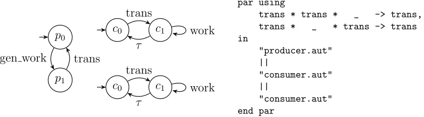
Example 1.An example of an LTS network can be found in Figure 2.1. This network contains one producer and two consumers. After the producer generates work (action gen work), the work is sent to one of the two consumers by synchronizing on thesend action. The consumer that received the work, processes it (action work), until at some point it is ready to receive new work. The synchronization rules are specified using the EXP syntax on the right. The two synchronization rules represent the transmission of work to the first and second consumer respectively. An underscore indicates that a process does not synchronize based on that rule.

For every network, we can define an LTS that represents its state space.

Definition 3. Let N = (Π, V) be a network of processes. TN = (S, A, τ,sˆ) is the LTS induced by this network, where:

• S=S[1]× · · · ×S[n] is the cross-product of all the state spaces.

• A=A[1]∪ · · · ∪A[n] is the union of all actions sets.

• τ = {(hs1, . . . , sni, a,hs01, . . . , s0ni)|∃(~t, a) ∈ V.∀i ∈ {1, . . . , n}.~t(i) = 1 ⇒ (si, a, s0i) ∈ τi ∧~t(i) = 0 ⇒ si = s0i} ∪ {(hs1, . . . , sni, a,hs01, . . . , s

0

ni)|∃i ∈

(12)

p0

p1

c0 c1

gen work trans

trans

work

τ

trans

work

τ

par using

trans * trans * _ -> trans, trans * _ * trans -> trans in

"producer.aut" ||

"consumer.aut" ||

[image:12.612.96.516.96.212.2]

"consumer.aut" end par

Figure 2.1: Example of LTS network with one producer and two consumers.

• ˆs = hsˆ[0], . . . ,sˆ[n]i is the initial state, which is a combination of the initial states of the processes.

The states of TN are vectors with n slots. The ith slot in a states is calleds[i]. We refer to each of the fields of process Π[i] with S[i],A[i],τ[i] and ˆs[i] respectively. The actions of process Π[i] that are enabled in statesare referred to asenabledi(s) = enabled(s[i]).

2.2 Exploration

Since the set of reachable states of a process network is restricted by the synchro-nization rules in most cases, it is hard to predict whether it contains some error state or other undesired behaviour. To decide this problem, the whole set of reachable states has to be constructed on a state-by-state basis, starting with the initial state. This is computationally a hard problem, due to the fact that the size of the state space grows exponentially with the amount of processes. This phenomenon is called state-space explosion.

A detailed procedure for state-space exploration is listed in Algorithm 1. States are stored in two sets: all the states that still need to be explored are in Open and all the states for which exploration has at least started are inClosed. On lines 2 and 3, one state s is selected from Open and moved to Closed. Then, all the successors of s that have not been explored yet are added to Open (line 6). The algorithm terminates when there are no states left to explore.

(13)

Algorithm 1: State-space exploration algorithm

Data: Open← {sˆ}, Closed← ∅ 1 whileOpen6=∅do

2 Open←Open\ {s} for some s∈Open; 3 Closed←Closed∪ {s};

4 foreacht∈succ(s)do

5 if t /∈Closed then

6 Open←Open∪ {t};

2.3 Partial-Order Reduction

To combat the state-space explosion, several reduction techniques have been pro-posed [38, 26, 35]. The general concept of reductions can be formally defined using areduction function.

Definition 4. A reduced LTS can be defined according to some reduction function

r:S →2A_{. The reduction of}_T _{according to}_r _{is denoted by}_T

r = (Sr, A, τr,sˆ), such that:

• (s, α, t)∈τr if and only if (s, α, t)∈τ and α∈r(s).

• Sr is the set of states reachable from ˆs under τr.

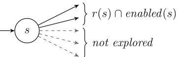
As we can see, for each reduction function r and transition system T, there is a unique reduced system Tr. Clearly, Tr does not depend on the way that r was computed. Although it is possible to compute the reduction function after generating the whole state space, this does not solve the problem of state-space explosion. We would likely run into memory limitations before the state-space generation even completed. Another option is to compute some restrictions on r beforehand [28]. However, this technique may offer significantly less reduction [34]. Therefore, the preferred solution is to compute the reduction function while generating the state space (on-the-fly). In that case, we decide which actions to preserve and which actions to prune at the moment a state is explored. The states to which the pruned actions lead are not explored at that time (see Figure 2.2). However, these states may be explored later if they are reachable through other transitions. The downside of performing some reduction algorithm on-the-fly is that there is no overview of the whole state space. Therefore, the choice for r(s) is usually not optimal.

(14)

s

r(s)∩enabled(s)

[image:14.612.374.479.92.200.2]

not explored

Figure 2.2: Transitions that are not defined under the reduction function

r are not explored.

s0

s1 s2

s3

α β

β α

Figure 2.3: LTS with two indepen-dent actions α and β.

suffices to check only some of those interleavings. To reason about this, we define when actions areindependent.

Definition 5. Two actions α, β, with α 6=β are independent in state s if and only if the following conditions hold:

• if β ∈enabled(s), then α∈enabled(s)⇔α∈enabled(succ(s, β))

• if α∈enabled(s), then β ∈enabled(s)⇔β ∈enabled(succ(s, α))

• succ(succ(s, α), β) =succ(succ(s, β), α)

Actions that are not independent are called dependent.

Example 2. We consider a system where one process reads a variable x (action

α) and another process writes variable y (action β). These actions are globally independent, because the order in which they are executed does not influence the result. This can be represented visually as in Figure 2.3. We call this a diamond structure.

From any execution in the system, we can obtain other interleavings by repeatedly permuting adjacent independent actions.

Example 3. Letαβ1β2 be an action sequence inT, whereα is globally independent

of β1 and β2. Then β1αβ2 and β1β2α are also action sequences in T. On the other

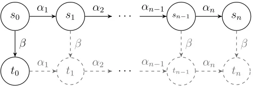
[image:14.612.97.277.122.180.2]

(15)

s0 s1 · · · sn−1 s_n

t0 t1 · · · tn−1 t_n

β

α1 α2 αn−1 αn

β β β

[image:15.612.177.436.94.185.2]

α1 α2 αn−1 αn

Figure 2.4: By repeatedly applying the persistence condition (C1) to the path

s0. . . si, where 0 < i ≤ n, we can conclude that states t1. . . tn exist. Therefore, C1 enforces that we can only choose r(s0) = {β} when β is independent of all αi for 0< i≤n. In this way, the persistence condition is prevents loss of behaviour.

2.3.1 Persistent Sets

Based on the theory of independent actions and their interleavings, the following restrictions on the reduction function have been defined [12, 37]:

C0a r(s)⊆enabled(s).

C0b r(s) = ∅ ⇔enabled(s) =∅.

C1 For all s ∈ S and executions s α1

−→ s1

α2

−→ . . . −−−→αn−1 sn−1

αn

−→ sn such that

α1, . . . , αn ∈/ r(s), αn is independent in sn−1 with all actions inr(s).

C0a and C0b make sure that the reduction does not introduce new behaviour and new deadlocks respectively. C1 implies that all α ∈ r(s) are independent of enabled(s) \r(s). Informally, this means that only the execution of independent actions can be postponed to a later state (cf. Figure 2.4). A set of actions that satisfies these criteria is called a persistent set. It is hard to compute the smallest persistent set, therefore several practical approaches have been proposed, which will be introduced in Chapter 4.

Any persistent set preserves deadlocks and can therefore be used to check a system for deadlocks. However, we are also interested insafety properties, which are generally not preserved. Therefore, we have to address another issue: the action-ignoring problem.

2.3.2 Action Ignoring

(16)

s0

s1

s2

α1

α2

α3 ||

t0

t1

β =

s0t0

s1t0

s2t0

s0t1

s1t1

s2t1

[image:16.612.154.467.92.245.2]

α1 α2 α3 α1 α2 α3 β β β

Figure 2.5: Indefinite ignoring of action β.

that is not part of r(s) for any state s ∈ Tr. Because we are dealing with finite state-spaces and we have to satisfy condition C0b, this can only happen in a cycle.

Example 4. In Figure 2.5, we see the parallel composition of two processes. In the parallel composition, action β is ignored indefinitely along one of the loops, which leads to statess0t0, s1t1 and s2t1 never being explored.

In order to preserve safety properties, we need to impose another condition on the reduction function. This condition is called the action ignoring proviso and it prevents actions from being postponed for ever.

C2ai For every state s∈Sr and every action α ∈enabled(s), there exists an execu-tion s α1

−→s1

α2

−→. . . αn

−→sn in the reduced state space, such thatα∈r(sn).

By preventing ignoring of actions, any transition label that occurs in the original state space, also occurs in the reduced state space [38]. Therefore, violations of safety properties (indicated by a special error transition either in one of the processes or in an additional monitor process) are also preserved. Note that other temporal properties are not preserved, but they fall outside of the scope of this thesis.

The problem with the action ignoring proviso is that it requires an overview of the reduced state-space. Moreover, the problem of finding the minimal amount of states covering all cycles is NP-complete. Therefore, it is not possible to apply these provisos directly in an on-the-fly POR algorithm.

Provisos for Safety Properties

(17)

it is possible to further postpone the execution of some action. As an example, we consider POR under depth-first search. When a certain states is expanded and we find a transition leading back to a state that is on the DFS stack, we have found a cycle. In case all actions in r(s) lead back to the stack, this might result in action-ignoring. In that case we should either try to find another set of actions for our reduction or fully expand s. This strategy is formally defined in condition C2s (C2-stack):

C2s There is at least one action α ∈r(s) and state t such that s −→α t and t is not in the DFS stack. Otherwise,r(s) =enabled(s).

Condition C2s implies C2ai [11], therefore C2s prevents the ignoring of actions. For algorithms that do not follow a DFS order, the following, more generalclosed-set proviso [12] can be used as an alternative for C2s.

C2c There is at least one actionα∈r(s) and statetsuch thats −→α tandt /∈Closed. Otherwise,r(s) =enabled(s).

2.4 GPU Architecture

CUDA is a programming interface developed by NVIDIA to enable general purpose programming on a GPU [1]. It provides a unified view of the GPU (‘device’), sim-plifying the process of developing for multiple devices. Code to be run on the device (‘kernel’) can be programmed using a subset of C++. The kernel specifies the be-haviour of a single thread. When the kernel is executed, multiple threads execute the same code in parallel.

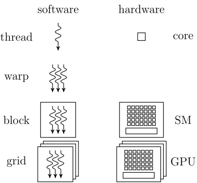
Considering the hardware, a GPU is divided up into several streaming multi-processors (SM) that each contain a large amount of cores. On the side of the programmer, threads are grouped into blocks. When assigning work to a GPU, the number of threads per block and the number of blocks need to be specified. The GPU then schedules the thread blocks on the streaming multiprocessors. One SM can run multiple blocks at the same time, but one block cannot execute on more than one SM. The SM manages threads in groups of 32 threads, calledwarps. Threads in a warp execute instructions in lock-step fashion. Figure 2.6 provides an overview of the software and hardware thread hierarchy.

(18)

software hardware

thread core

warp

block SM

[image:18.612.206.407.94.281.2]

grid GPU

Figure 2.6: Summary of software and hardware thread hierarchy in CUDA.

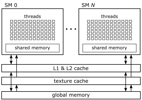
in that block. The shared memory is placed on-chip, therefore it has a low latency. Secondly, there is the global memory that can be accessed by all the threads. It has a high bandwidth, but also a high latency. The amount of global memory is typically multiple gigabytes. There are three caches for the global memory: the L1 cache, the L2 cache and the texture cache. Data in the global memory that is marked as read-only (a ‘texture’) may be placed in the texture cache. The global memory can also be accessed by the CPU (‘host’), thus it serves as an interface between the host and the device. Figure 2.7 provides a schematic overview of the architecture.

The key to writing efficient GPGPU programs is making optimal use of the ar-chitecture. The work should be divided into small tasks that will be executed by the thread blocks. All threads in a block work together on this small task. The work division strategy plays an important role, because communication between blocks is only possible via global memory. Therefore, data dependencies between blocks should be avoided.

Warps influence the performance of GPU algorithms in several ways. Firstly, the amount of branch divergence within warps should be kept to a minimum. Consider an if-statement with condition C, where C is true for at least one thread and false for at least one thread. Since the threads in one warp step through all instructions together, the two branches will be executed sequentially. This can lead to a reduction in performance.

(19)

shared memory threads

SM 0

shared memory threads

SM N

[image:19.612.193.419.90.249.2]

L1 & L2 cache texture cache global memory

Figure 2.7: Schematic overview of the GPU architecture.

from global memory, this memory access can be executed in parallel. This is called coalesced access. Additionally, this data fits exactly in one cache line of 128 bytes.

Finally, there are several instructions for quickly exchanging data between threads of a warp. Thesewarp instructions are implemented by register swapping. CUDA’s memory model does not guarantee visibility of writes without a barrier synchroniza-tion, even between threads of the same warp. Therefore, it is often faster to apply warp instructions and avoid synchronization of the whole block.

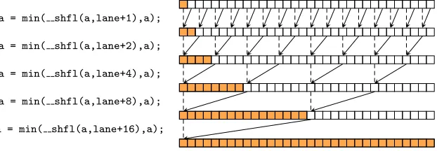
Example 5. Figure 2.8 illustrates how warp instructions enable fast data sharing. Here, we will compute the minimum value of a variable a of all threads in a warp using butterfly reduction. For this reduction algorithm, the shuffle instruction is used. This function has two arguments: the first argument is the value to exchange and the second argument is the source lane (index of a thread in its warp). It returns the value of the first argument as computed by the source lane. For this algorithm, we compute the source lane by applying an offset. After each shuffle operation, the minimum value of variablea is recomputed and the offset is increased by a factor two. In this way, we achieve a tree-like structure for the data exchanges and only five instructions are necessary to compute a minimum from the variables of 32 threads. Although Figure 2.8 only displays the information flow relevant for the first thread, the same algorithm is executed by all threads in a warp. Therefore, when the algorithm terminates, all 32 threads have computed the same minimum value.

(20)

a = min( shfl(a,lane+1),a);

[image:20.612.155.466.95.203.2]

Figure 2.8: Computing the minimum of variable a over all threads of one warp with butterfly reduction. The flow of data relevant for the first thread of the warp (lane = 0) is indicated by the arrows. Of course, variable a also carries over between iterations, as indicated by dashed lines. The value of variable a for the first thread is the minimum of all as of the orange-coloured threads after each step.

(21)

Chapter 3 Optimizations

This chapter first introduces the existing architecture of GPUexplore. Then, it dis-cusses how we optimized the implementation to minimize the runtime required for state-space exploration.

3.1 Existing Design

GPUexplore is a model checker that can check for deadlocks and safety properties. GPUexplore executes all the computations on the GPU and does not rely on any processing by the CPU. The main kernel of GPUexplore implements lines 2-6 of Algorithm 1. This kernel is launched repetitively until all states have been explored. The Open and Closed set are implemented by a single hash table that occupies most of the global memory. All states are stored in this hash table. Whether a state is new (in theOpen set) or old (in the Closed set) is indicated by a single bit in the state vector. This bit is not considered by the hash function. This ensures that a state will be inserted in the same position, regardless of the value of the new/old bit. The hash table uses open addressing with rehashing. Since we are not interested in deleting states from the hash table, it only needs to support afindOrPut operation. This operation tries to find an element, and if it is not present, the element is inserted. The implementation of findOrPut is thread-safe: it does not allow for data races. In addition, it is lock-less: the atomic compareAndSet (CAS) operation is used to guarantee thread-safety. The hash table is divided into buckets of 32 integers. Each bucket may contain multiple state vectors. Whenever possible, threads cooperate with the other threads in their warp and read/write a complete bucket to ensure coalesced access.

(22)

As described in section 2.4, the hardware enforces that threads are grouped in warps of size 32. We also created logical groups, called vector groups (note that vector groups are not a CUDA concept). The number of threads in a vector group is equal to the number of processes in the network (cf. section 2).The threads in a vector group cooperate to compute the successors of a single state. Each thread has a vector group thread index (vgtid) and is responsible for generating the successors of process Π[vgtid]. Successors following from synchronizing actions are generated in cooperation. Threads with vgtid 0 are group leaders. Note that the algorithms presented here specify the behaviour of one thread, but are run on multiple threads and on multiple blocks. Most of the synchronization is hidden in the functions that access shared or global memory.

Algorithm 2: GPUexplore exploration framework

Data: global table[ ]

Data: shared workTile[ ], cache[ ]

1 vgid←tid / numP roc; /* index of the vector group */

2 vgtid←tidmodnumP roc; /* id of the thread in the group */

3 foreachi∈0. . ._{NumIterations}do 4 workT ile←gatherWork(); 5 syncthreads();

6 s←workT ile[vgid]; 7 foreacht∈succvgtid(s)do

8 storeInCache(t); 9 syncthreads(); 10 foreacht∈cache do 11 if isNew(t)then 12 findOrPutWarp(t);

13 markOld(t);

A high-level view on the algorithm of GPUexplore is presented in Algorithm 2. This kernel is executed repetitively until all reachable states have been explored. In between two kernel launches, the CPU only queries the GPU to determine whether exploration has finished. Several kernel iterations may be performed during each launch of the kernel (NumIterations is set by the user). Each iteration starts

withwork gathering: blocks search for unexplored states in global memory and copy those states to the work tile in shared memory (line 4). Once the work tile is full, the

(23)

placed in a cache in shared memory (line 8). When all the vector groups in a block are done with successor generation, each warp scans the cache for new states and copies them to global memory (line 12). The states are then marked old in the cache (line 13), so they are still available for local duplicate detection later on. For details on how successors are computed and the inner workings of the hash table, we refer to [42].

3.2 Improvement of Work Scanning

At the beginning of each iteration, each block fills its work tile by linearly scanning the hash table in global memory (cf. Algorithm 3). Each warp linearly scans its section of the hash table by stepping a nrOfWarps amount of buckets in each iteration (line 14). When a new state is found (line 9), the amount of states in the work tile (stored in tileCount) is incremented atomically (line 10). If the previous value of tileCount (stored in j) is smaller than the size of the work tile (line 11), then the state is copied from the hash table into the work tile and marked as old in the hash table (lines 12-13).

Algorithm 3: Work gathering

Data: shared workTile[ ], tileCount

1 functiongatherWork():

2 lane←threadIdmodwarpSize; 3 warpId←threadId/warpSize;

4 globalW arpId←(nrOfBlocks/warpSize)∗blockId+warpId; 5 nrOfWarps ←(blockSize/warpSize)∗nrOfBlocks;

6 i←globalW arpId;

7 whilei <|table| ∧tileCount < blockSize/nrP rocsdo 8 s←table[i∗warpSize+lane];

9 if isNew(s)then

10 j←atomicInc(&tileCount);

11 if j < blockSize/nrP rocsthen

12 workT ile[j]←s;

13 markOld(table[i∗warpSize+lane]);

14 i←i+nrOfWarps;

[image:23.612.91.534.371.591.2]

(24)

claim-ing: at the end of each iteration, when copying new states from the cache to global memory, blocks can immediately place these in their work tile. This saves time when scanning for work in the next iteration. In the case that a block manages to fill the entire work tile, it even avoids work scanning completely.

This technique can not be applied during the last iteration of a kernel launch, however, since the contents of shared memory are lost after the termination of a kernel. To solve this problem, we copy the contents of the work tile to global memory after the last iteration. Before the first iteration of the next kernel launch, we copy this information back to the work tile in shared memory.

The second improvement we made is to save the location where the previous scan terminated. During the next iteration, we will start scanning from that location. Suppose the hash table was scanned until location n during the previous iteration. In that case, the locations 0 ≤ globalW arpId+k ∗nrOfWarps < n, for all k ∈ _N, only contain new states that were inserted between the previous scan and this scan. Therefore, it is more efficient to continue scanning at locationn.

The third optimization is to track whether work is available for a block: for every block, there is a flag that indicates whether the part of the hash table scanned by that block contains a new state. The flags are stored in global memory, so they can be accessed by all threads. Initially, all flags are set to false. Whenever a new state is inserted into the hash table, the flag of the block corresponding to the location of the state is set to true. When a block scans its part of the hash table and finds no new states, it sets its flag tofalse. Blocks will not try to scan the hash table for new states when their flag is set tofalse. This optimization carries some overhead, due to the increased amount of accesses to global memory. However, blocks no longer scan the hash table unnecessarily. The benefit becomes greater as the hash table becomes larger.

The final, small optimization in this area is to avoid scanning the cache (line 10 of Algorithm 2) when the work tile is empty. In that case, no states have been gathered, no successors have been generated and thus the cache is empty.

3.3 Hash Table

(25)

Therefore, we have improved the hash function (Algorithm 4). The new imple-mentation first sums all integers of the state vector, while applying some bit shifts in between (line 3). Then, it multiplies with a hash constanta, adds a constant b and computes the modulo with respect to P, where P is a large prime number (line 4). Finally, the position in the hash table is computed by taking the modulo with respect to the number of buckets.

We have empirically determined that this hash function offers a good trade-off between runtime and the amount of hash collisions. It leads to a good spread of states in the hash table.

Algorithm 4: Improved hash function

Input: constanta,constant b,constantP, nr buckets, state[ ]

Output: hash

1 hash←0;

2 foreachs∈state[ ]do

3 hash←(hash + s)<<5;

4 hash←((a*hash+b) mod P) mod nr buckets;

This hash function can slightly improve the runtime of the state-space explo-ration. Since states are spread better through the hash table, finding a fully oc-cupied bucket on the first try is less likely. Therefore, less rehashing is required. Furthermore, we changed the implementation to avoid costly 64 bit modulo opera-tions whenever possible.

The second improvement related to the hash table is the removal of all single-threaded accesses to the hash table. In the original implementation, whenever the cache was full, a thread may insert states directly into the hash table in global mem-ory by itself. This single-threaded implementation was sensitive to race-conditions, however, resulting in duplicate entries in the hash table. By exchanging data with warp instructions, it is possible to use the warp version of findOrPut instead. This implementation provides coalesced access, so it helps to speed-up exploration in those cases where the cache overflows.

3.4 Branch Divergence and Synchronization

(26)

In the original version of GPUexplore, vector groups and warps were not related in any way. This means that a vector group can be part of more than one warp. To bring the threads of a vector group in sync required a call to the syncthreadsfunction from the CUDA API, which forces the whole block to synchronize. This caused a lot of unnecessary waiting. Therefore, we restructured the thread layout, so that a vector group will never cross a warp boundary. A warp may still contain multiple vector groups, however. This allows us to perform most of the communication between threads via warp instructions and to remove all calls to syncthreads from the main loop of the kernel. This greatly speeds up successor generation, since threads spend less time waiting for each other.

3.5 Generating Synchronizing Transitions

The generation of successors (lines 7 and 8 of Algorithm 2) has also been optimized. In the original design of Wijs and Boˇsnaˇcki [42], finding the action with the smallest label index was done by the group leader, which scanned the buffer of each of the threads in the group. Next, the synchronizing transitions for the action with the smallest label index were generated.

First, we replaced the sequential buffer scanning by butterfly reduction through warp instructions (cf. section 2.4) to find the smallest label index. Since we only have to find the minimum within the vector group, this requiresdlog₂newarp instructions, wheren is the number of processes in the network.

(27)

Chapter 4 Partial-Order Reduction

This chapter explains the details of the implementation of partial-order reduction in GPUexplore. First, it discusses how GPUexplore can be extended with partial-order reduction. Then, a formal proof is provided to show that the proposed algorithms are correct.

Before we explain the extensions required to implement partial-order reduction, it is important to note that the search order of GPUexplore is not strictly DFS or BFS. GPUexplore does not implement a stack or a queue to enforce a work order, but gathers states from global memory. Therefore, the search algorithm should be categorized asgeneral state expanding algorithm (GSEA) [17]. We satisfy the action ignoring proviso by implementing the GSEA cycle proviso that was introduced by Boˇsnaˇcki et al. [12].

In literature, multiple practical approaches to partial-order reduction have been proposed. The GPU implementation of ample sets [37, 24], cample sets [8] and stubborn sets [38] is discussed below. Sleep sets have not been considered, since they require a large amount of memory for each state.

In the following sections, we will explain how lines 7 and 8 of Algorithm 2 can be adjusted to implement POR.

4.1 Ample-set Approach

(28)

Algorithm 5: Successor generation under the ample-set approach

Data: shared cache[ ], buf[ ][ ], reduceProc[ ]

1 functiongenerateSuccessors():

2 bufCount ←0,reduceP roc[vgid]←numP rocs; 3 if processHasOnlyLocalT rans(s, vgtid)then 4 foreacht∈succvgtid(s)do

5 location←storeInCache(t);

6 buf[tid][bufCount]←location;

7 bufCount ←bufCount+ 1;

8 foreachi∈[0..bufCount−1]do 9 j←findGlobal(cache[buf[tid][i]]); 10 if j=_NotFound∨isNew(table[j])then

11 atomicMinimum(&reduceP roc[vgid], vgtid); 12 syncthreads();

13 if reduceP roc[vgid]< numP rocs∧reduceP roc[vgid]6=vgtidthen 14 foreachi∈[0..bufCount−1]do

15 markOld(cache[buf[tid][i]]); 16 syncthreads();

17 if reduceP roc[vgid] =vgtidthen 18 foreachi∈[0..bufCount−1]do 19 markNew(cache[buf[tid][i]]); 20 if reduceP roc[vgid]≥numP rocsthen

21 /* generate the remaining successors */

actions are safe, so reduction can only be applied if we find a process with only local actions enabled.

(29)

chance to mark their states as new if they have been marked as old by a thread from another vector group (line 19). In case no thread can apply reduction, the algorithm continues as normal (line 21). Why states need to be marked as new will be explained in section 4.4.

4.2 Cample-set Approach

In our definition of a network of LTSs, local actions represent internal process be-haviour. Since most practical models frequently perform communication, they have only few local actions and consist mainly of synchronizing actions. The ample-set approach relies on local actions to achieve reduction, so it often fails to reduce the state space. To solve this issue, we implemented cluster-based POR [9]. Contrary to the ample-set approach, all actions of a particular set of processes (the cluster) are selected. The notion of safe actions is still key. However, the definition is now based on clusters. An action is safe with respect to a clusterC ⊆ {1, . . . , n}(n is the number of processes in the network), if it is part of a process of that cluster and it is independent of all actions of processes outside the cluster. Now, for any cluster C

that has only actions enabled that are safe with respect toC,r(s) =S

i∈Cenabledi(s) is a valid cluster-based ample (cample) set. Note that the cluster containing all processes always yields a valid cample set.

Whereas Basten and Boˇsnaˇcki [9] determine a tree-shaped cluster hierarchy a priori and by hand, our implementation computes a cluster on-the-fly for every in-dividual state. This should lead to better reductions, since the fixed hierarchy only works for parallel processes that are structured as a tree. Dynamic clustering works for any structure, for example ring or star structured LTS networks. In [9], it is argued that computing the cluster on-the-fly is an expensive operation, so it should be avoided. Our approach, when exploring a state s, is to compute the smallest clusterC, such that ∀i∈ C :C[i]⊆ C, whereC[i] is the set of processes that process

isynchronizes with in the state s. This can be done by running a simple fixed-point algorithm, with complexity O(n), once for every C[i] and finding the smallest from those fixed points. This gives a total complexity of O(n2_{). However, in our}

imple-mentation,nparallel threads each compute a fixed point for someC[i]. Therefore, we are able to compute the smallest cluster in linear time with respect to the amount of processes. Dynamic clusters do not influence the correctness of the cample-set approach, the reasoning of [9] still applies.

(30)

cycle proviso (we remind the reader that each thread is associated with exactly one process). Each thread starts by assigning the information obtained during successor generation tocluster andproviso(lines 2-3). After the work set of processes is initial-ized (line 5), some processi is selected from the work set (line 7). Then,i is added to the cluster of this thread (line 8) and the work set and proviso status is updated with the data fromi (lines 9-10). When every thread has finished computing the closure, the results are shared (lines 12-13). From all clusters, the group leader selects the smallest (line 16). This cluster is then returned by all threads in the group.

Algorithm 6: Algorithm for computing a cluster in parallel.

Data: shared cluster[ ], proviso[ ]

1 functiondetermineCluster(myCluster,provisoSatisfied): 2 cluster[vgtid]←myCluster;

3 proviso[vgtid]←provisoSatisfied; 4 syncthreads();

5 clW ork←myCluster; 6 whileclW ork6=∅ do

7 clW ork←clW ork\ {i}for somei∈clW ork;

8 myCluster←myCluster∪ {i};

9 clW ork←clW ork∪(cluster[i]\myCluster); 10 provisoSatisfied←provisoSatisfied∨proviso[i]; 11 syncthreads();

12 cluster[vgtid]←myCluster; 13 proviso[vgtid]←provisoSatisfied; 14 syncthreads();

15 if vgtid= 0then

16 selectedCluster←cluster[i]whereproviso[i]∧ |cluster[i]| ≤ |cluster[j]|for allj; 17 cluster[0]←selectedCluster;

18 syncthreads(); 19 returncluster[0];

(31)

all actions, we determine which processes may synchronize on that action and save this information inmyCluster (line 10). Then, the cluster is computed according to Algorithm 6 (line 11). Finally, states are marked as old (line 14) or new (line 14) depending on whether they follow from an action in the cample set.

Algorithm 7: Algorithm for generating states using a cample set.

Data: shared cluster[ ]

1 functiongenerateSuccessors(): 2 myCluster← {vgtid};

3 provisoSatisfied ←false;

4 foreacha∈enabled(s, vgtid)do 5 foreacht←succ(s, a)do 6 loc←storeInCache(t); 7 j←findGlobal(t);

8 if j =_NotFound∨isNew(table[j])then

9 provisoSatisfied←true;

10 myCluster←myCluster∪actionSyncsW ith(a); 11 cluster←determineCluster(myCluster,provisoSatisfied); 12 if vgtid∈clusterthen

13 foreacht∈successors(s, vgtid)do 14 markOld(cache[findInCache(t)]);

15 syncthreads(); 16 if vgtid /∈clusterthen

17 foreacht∈successors(s, vgtid)do 18 markNew(cache[findInCache(t)]);

4.3 Stubborn-set Approach

(32)

algorithm, since the amount of shared memory required is relatively high. However, this is the only design that results in an acceptable computational overhead.

To compute a stubborn set, we use several matrices that have been computed during pre-processing. Information about the dependency of actions is stored in the do-not-accord (DNA) matrix and information about how action can be enabled and disabled is stored in the necessary enabling set (NES) and necessary disabling set (NDS) matrices respectively. For more details on these matrices, we refer the reader to Laarman et al. [30]. To further reduce the size of the computed stubborn set, we apply the heuristic function from [30]. Contrary to their implementation, we do not compute a stubborn set for all possible choices of initial action. Effectively, we sacrifice some reduction potential in order to minimize the runtime overhead and the amount of memory required for computing a stubborn set.

(33)

Algorithm 8: Algorithm for generating states using a stubborn set.

Data: shared stubborn[ ][ ], work[ ][ ], enabled[ ][ ], proviso[ ][ ], continue[ ]

1 functiongenerateSuccessors(): 2 buildStubbornSet();

3 foreacha∈enabled(s, vgtid)do 4 if stubborn[vgid][a] then 5 foreacht←succ(s, a)do

6 storeInCache(t);

7 functionbuildStubbornSet(): 8 foreacha∈enabled(s, vgtid)do 9 enabled[vgid][a]←true; 10 foreacht←succ(s, a)do 11 j←findGlobal(t);

12 if j =_NotFound∨isNew(table[j])then

13 proviso[vgid][a]←true;

14 syncthreads();

15 if ¬proviso[vgid][a]for allathen 16 stubborn[vgid][a]←truefor alla; 17 return;

18 syncthreads(); 19 if vgtid= 0then

20 work[vgid][a]←truefor somea:proviso[vgid][a]; 21 continue[vgid]←true;

22 syncthreads(); 23 whilecontinue[vgid]do

24 act←afor somea:work[vgid][a]∧a=k∗num procs+vgtid; 25 work[vgid][a]←f alse;

26 stubborn[vgid][a]←true; 27 if enabled[vgid][a]then

28 atomicOr(&work[vgid],fetchTexture(DNA[a])∧¬stubborn[vgid]); 29 else

30 atomicOr(&work[vgid],fetchTexture(N[a])∧¬stubborn[vgid]) where

N←f ind nes heur(act);

31 syncthreads();

32 if vgtid= 0 then

33 continue[vgid]←f alse;

34 syncthreads(); 35 if actthen

36 continue[vgid]←true;

(34)

4.4 Proof of Correctness

In this section, we give a formal argument why the GPU POR algorithms we proposed are correct, i.e. why they produce a reduction function that satisfies the criteria of a persistent set.

4.4.1 Sequential correctness

First, we will prove that each of the POR algorithms we proposed produces valid persistent sets when run with minimal parallelism.

Theorem 1. Algorithm 5 produces a correct ample set that satisfies the action ig-noring proviso when run with minimal parallelism (using only one vector group of numProcs threads).

Proof. The algorithm can generate successors according to either of two results:

• All transitions of a process Π[i] that has at least one local transition and no synchronizing transitions (r(s) = enabledi(s)).

• All transitions (r(s) =enabled(s))

Since conditions C0 - C2 are trivially true for the second result, we will focus on the first outcome. C0a and C0b are again trivially true. In order to determine locally whether r(s) =enabledi(s) satisfies condition C1, we have to satisfy two conditions [2]:

C1a: Anyα∈A[j] is independent of enabledi(s) for i6=j.

C1b: Any α ∈ A[i]\enabled(s) may not become enabled through the activities of some process Π[j] with i6=j.

Because we chose a process with only local actions, all actions in enabledi(s) are independent of any α ∈ A[j] (C1a is satisfied). C1b is trivially satisfied: since enabledi(s) does not contain blocked actions, there is no action in Π[i] that can become enabled in any way. Therefore, we have satisfied C1b. We can now deduce that condition C1 is also satisfied.

(35)

These conditions together imply that the selected set of actions is indeed a correct persistent set (conditions C0 - C2) that satisfies the action ignoring proviso (condition C2).

As stated in the previous proof, we apply the local criteria from Baier and Ka-toen [2] for condition C1 to compute a valid ample set. In order to apply these criteria to cample sets, a slight generalization is needed. The following local criteria ensure that condition C1 is satisfied when we choose r(s) = S

i∈Cenabledi(s) for some cluster∅ 6=C ⊆ {1, . . . , n} of a network N.

C1c: Anyα∈A[j] is independent of S

i∈Cenabledi(s) forj /∈C.

C1d: Anyα ∈(S

i∈CA[i])\enabled(s) may not become enabled through the activities of some process Π[j] with j /∈C.

The accompanying lemma is also adapted (Baier and Katoen [2], lemma 8.27):

Lemma 1. If C1c and C1d hold, then r(s) = S

i∈Cenabledi(s) for some cluster

∅ 6=C ⊆ {1, . . . , n} satisfies condition C1 for all executions that start in s.

Proof. In caseC ={1, . . . , n}, C1 trivially holds. In other cases, the reasoning below applies.

Suppose that C1c and C1d hold, but C1 does not hold. Let sbe the state we are exploring. Because C1 does not hold, there exists an execution s −→α1 s1

α2

−→ . . .−α−→m

sm αm+1

−−−→, where α1, . . . , αm ∈/ r(s) (and therefore α1, . . . , αm ∈/

S

i∈Cenabledi(s)) and αm+1 depends on r(s). Because of condition C1c, any action that depends on

r(s) is an action of some process Π[i] with i∈C.

Let k be the largest index in {1, . . . , m} such that α1, . . . , αk−1 are actions of

processes not in C: α1, . . . , αk−1 ∈ S_{j /}∈CA[j]\

S

i∈CA[i] and αk ∈

S

i∈CA[i]. Be-cause the actions α1, . . . , αk−1 cannot change the state of any process Π[i] with

i ∈ C, states s1, . . . , sk−1 are the same as state s in all slots i ∈ C. αk ∈/ r(s) and αk ∈

S

i∈Cenabledi(sk−1), so action αk becomes enabled in some slot i ∈ C through the execution of one of the actions α1, . . . , αk−1. Since α1, . . . , αk−1 are

actions of processes Π[j] withj /∈C, this contradicts C1d.

Theorem 2. Algorithm 7 produces a correct cample set that satisfies the action ignoring proviso when run with minimal parallelism (using only one vector group of numProcs threads).

(36)

Theorem 3. Algorithm 8 produces a correct stubborn set that satisfies the action ignoring proviso when run with minimal parallelism (using only one vector group of numProcs threads).

Since our stubborn-set algorithm is not fundamentally different from the original sequential version, we refer to Theorem 4.18 of Godefroid [21] for the proof of this theorem.

4.4.2 Parallel correctness

The cache that is maintained in shared memory is read and modified by all threads. Therefore, our algorithms may no longer be correct when executed on multiple vector groups within one block. With the following theorem, we prove that this is not the case. The ample-set algorithm is used as an example, but the reasoning applies to all three implementations.

Theorem 4. Algorithm 5 produces a correct ample set when run using multiple vector groups within one block.

Proof. We consider two vector groups A and B that are member of the same block. From Theorem 1 we know that the result of each of the vector groups produces a correct ample set when run sequentially. When run in parallel, there are two ways in which the actions of group B can influence the result of group A.

• Vector group A does not apply reduction. However, group B marks some of the states in the buffer of group A as old. This may lead to an unwanted loss of states.

• Vector group A applies reduction by marking states in the cache as old (line 15). However, group B later marks some or all of these states asnew (line 19). This makes the group of selected transitions for A larger, possibly affecting correctness.

In the first situation, the actions of group B are negated, because group A marks all the successors it found asnew after B marked them asold. Therefore, the correctness of the result of group A is not affected.

(37)

s0 si

sj _t

β β

β

[image:37.612.169.440.100.192.2]

β

Figure 4.1: ‘Lasso’ shaped path from the proof of Lemma 2

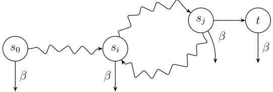
Blocks communicate with each other via global memory. For partial-order reduc-tion, the only relevant access to global memory happens at line 10 of Algorithm 5. We will now show that the correctness of our algorithms is not affected when running on multiple blocks. First, we introduce a new version of the cycle proviso and show that it implies the action-ignoring proviso.

Lemma 2. (closed-set cycle proviso) If a reduction algorithm satisfies conditions C0a, C0b and C1 and for every cycle s0

α0

−→ s1

α1

−→. . .−−−→αn−1 sn αn

−→s0 in the reduced

state space with β∈enabled(s0) andβ =6 αi for all 0≤i≤n, selects (i)at least one transition labelled withβ or (ii) at least one transition that, during the generation of the reduced state space, led to a state outside the cycle that has not been explored yet (i.e. ∃i∃(si, γ, t)∈τ :γ ∈r(si)∧t /∈Closed); then condition C2ai is satisfied.

Proof. Suppose that action β ∈ enabled(s0) for some s0 ∈ Sr is always ignored, i.e. condition C2ai is not satisfied. This means there is no execution s0

α0

−→ s1

α1

−→

. . . −−−→αn−1 sn β

−

→ t where αi ∈ r(si) for all 0 ≤ i < n. Because we are dealing with finite state spaces, every execution that infinitely ignores β has to end in a cycle. These executions have a ‘lasso’ shape, they consist of an initial phase and a cycle. Lets0

α0

−→ s1

α1

−→. . .−−→αi−1 si αi

−→. . .−−−→αn−1 sn αn

−→si be the execution with the longest initial phase, i.e. with the highest value i (see Figure 4.1). Since condition C1 is satisfied,β is independent of any αk and thus enabled on anysk with 0≤k ≤n. It is assumed that for at least one of the states si. . . sn an action exiting the cycle is selected. Letsj be such a state (i≤j ≤n). Sinceβ is ignored, β /∈r(sj). According to the assumption, one of the successors found throughr(sj) has not been inClosed. Let this state bet. Any finite path starting with s0. . . sjt cannot end in a deadlock without taking action β at some point (condition C0b). Any infinite path starting with s0. . . sjt has a longer initial phase (after all j+ 1 > i) than the execution we assumed had the longest initial phase. Thus, our assumption is contradicted.

(38)

evaluated on a per-state basis, the newclosed-set cycle proviso is a global property. Although the new proviso assumes C0a, C0b and C1, it can allow smaller reduction functionsr, since only one transition per cycle is required to lead to a state outside Closed.

Before we start the next proof, it is important to note three things. Firstly, the work gathering function on line 4 of Algorithm 2 moves the gathered states from

Open to Closed. Secondly, the working of the algorithm with respect to conditions C0a, C0b and C1 is not affected when it executes on multiple blocks. Finally, we again use our ample-set algorithm as an example, but the theorem applies to all three algorithms.

Theorem 5. Algorithm 5 produces a correct ample set that satisfies the cycle proviso when run on multiple blocks.

Proof. Lets0

α0

−→s1

α1

−→. . .−−−→αn−2 sn−1

αn−1

−−−→s0 be a cycle in the reduced state space.

In case α0 is dependent on all other enabled actions in s0, there is no action to be

ignored and C2ai is satisfied.

In case there is an action in s0 that is independent of α0, this action is prone

to ignoring. Let us call this action β. Because condition C1 is satisfied, β is also enabled in the other states of the cycle: β ∈enabled(si) for all 0≤i < n.

We now consider the order in which states on the cycle can be explored by multiple blocks. Letsi be one of the states of this cycle that is gathered from Open first (line 4, Algorithm 2). There are two possibilities regarding the processing of statesi−1:

• It is gathered fromOpen at exactly the same time as si. When the processing forsi−1 arrives at line 10 of Algorithm 5, it will findsi in Closed.

• It is gathered later thansi. Again, si will be inClosed.

Since si is in Closed in both cases, at least one other action will be selected for

r(si−1). If all successors ofsi−1 are in Closed, then β has to be selected. Otherwise,

at least one transition to a state that is not inClosed will be selected. Now we can apply Lemma 2.

Combining the obtained results gives us the following corollary:

Corollary 1. Algorithms 5, 7 and 8 produce a correct persistent set that satisfies the cycle proviso when run with multiple vector groups on multiple blocks.

(39)

Chapter 5 Experiments

This chapter presents the results of several experiments. First, it shows the speed-up gained by the optimizations proposed in Chapter 3. Second, the performance of the proposed POR algorithms is determined.

5.1 Speed-up of Optimizations

The optimizations that we proposed in Chapter 3 have been implemented in GPUexplore. We call this version GPUexplore 2.01_{. We want to determine the speed-up offered by}

the optimizations over the original version from [42]. Additionally, we will compare the performance with a traditional sequential model checker.

The models that were used as benchmarks (22 in total) have different origins.

Cache,sieve,odp, transit, asyn3 and desare all EXP models from the examples included in the CADP toolkit [20]. The leader election, anderson, lamport,

lann, peterson and szymanski models come from the BEEM database2 _{and have}

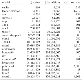
been translated from DVE to EXP. 1394, acs and wafer stepper are originally mCRL2 [15] models and have also been translated by hand to EXP. broadcast has been created by Wijs and Boˇsnaˇcki [42]. The models with a .1-suffix are enlarged versions of the original models [42]. The details of the models can be found in Table 5.1. ‘stub. set size’ indicates the maximum size of the stubborn set, which is relevant for the POR experiments. Since the stubborn set size mainly depends on the synchronization rules, it also gives an indication of the amount of synchronization rules in the network.

1_{Sources are available from https://github.com/ThomasNeele/GPUexplore}

(40)

[image:40.612.164.447.121.398.2]

Table 5.1: Overview of the models used in the benchmarks

model #states #transitions stub. set size

cache 616 4,631 222

leader election1 4,261 12,653 4,712

acs 4,764 14,760 134

sieve 10 23,627 84,707 941

odp 91,394 641,226 464

1394 198,692 355,338 301

acs.1 200,317 895,004 139

transit 3,763,192 39,925,524 73

wafer stepper.1 3,772,753 19,028,708 880

odp.1 7,699,456 31,091,554 556

1394.1 10,138,812 96,553,318 300

asyn3 15,688,570 86,458,183 1,315

anderson6 18,206,917 86,996,322 786

lamport8 62,669,317 304,202,665 305

des 64,498,297 518,438,860 12

szymanski5 79,518,740 922,428,824 481

broadcast 105,413,504 1,264,962,048 70

peterson7 142,471,098 626,952,200 2,880

lann6 144,151,629 648,779,852 48

lann7 160,025,986 944,322,648 48

asyn3.1 190,208,728 876,008,628 1,363

For all our experiments with GPUexplore 2.0, we use an NVIDIA Titan X, which was released in 2015. The Titan X has 24 SMs each with 128 CUDA cores, giving a total of 3072 CUDA cores. Each SM has 96KB of shared memory and the global memory has a size of 12GB. We allocate 5GB of the global memory for the hash table.

Before we compare our implementation to other implementations, we have to determine which parameter values give the best performance. There are two param-eters that can be tuned for optimal performance: the amount of iterations per kernel launch (K) and the amount of blocks (B). We fix the amount of threads per block (T) to 512, since any other value reduces the occupancy of the GPU.

We start by determining the optimal number of iterations per kernel launch. We run GPUexplore with 6144 blocks and 5GB allocated for the hash table and vary K between 1 and 32. The results can be found in Figure 5.1. When varying K between 1 and 4, the runtime for the majority of models does not change significantly. For higher K up to 32, a clear upward trend in runtime is visible. Only odp.1 and des

(41)

1 2 4 8 16 32 0.5

0.7 1 1.5 2 3 4 5 6

Number of kernel iterations (K)

[image:41.612.112.499.92.335.2]

Run time relativ e to K=1 cache le1 acs sieve odp 1394 acs.1 transit wafer odp.1 1394.1 as3 and6 lp8 des sz5 brcst pt7 lann6 lann7 as3.1

Figure 5.1: Runtime while varying the amount of kernel iterations (6144 blocks)

other models: it contains one very large process and several smaller ones. For the following experiments, we will fix K to one, since it gives the best performance for most of the models.

The fact that a high value for K causes a high runtime can be explained by the synchronizing effect of a kernel launch: at the end of a launch, the CPU waits until all GPU blocks are finished executing. At the beginning of the next launch, all memory writes from previous launches are guaranteed to be visible. This reduces the amount of work scanning needed. There is no function available in the CUDA API to replace the synchronization offered by a kernel launch. In [42], ten iterations per kernel launch yielded optimal performance. Since we have reduced the overhead of a kernel launch by temporarily storing the work tile in global memory (cf. section 3.2), the performance can be increased by performing a kernel launch more often, and thus synchronize the blocks more often.

Next, we will optimize the amount of blocks that the kernel runs on. With our kernel, an SM requires two blocks to be fully occupied and since the Titan X has 24 SMs, we vary B from 48 to 49152. The results are plotted in Figure 5.2.

(42)

48 96 192 384 768 1536 3072 6144 12288 24576 49152

1 10

Number of blocks (B)

[image:42.612.113.497.90.335.2]

Run time relativ e to B=6144 cache le1 acs sieve odp 1394 acs.1 transit wafer odp.1 1394.1 as3 and6 lp8 des sz5 brcst pt7 lann6 lann7 as3.1

Figure 5.2: Runtime while varying the amount of blocks (1 kernel iteration)

factor influencing the speed-up, is the fact that the availability of work is tracked on a per-block basis. As we increase the amount of blocks, each work available flag covers a smaller part of the hash table. Fine-grained work available flags help to prevent more unnecessary work scanning. When the amount of blocks is very high, the distribution of work between blocks becomes uneven. This especially affects the small models. Only the broadcast model benefits from a high amount of blocks. From these results, we can conclude that 6144 blocks and one iteration per kernel launch are the parameters that give the best performance.

Since the odp.1 and des model show different behaviour from the other models when varying either parameter, we will further study the parameter space for those models. The results are displayed in Figure 5.3. The best result for odp.1 (1.36 seconds) is achieved with 6144 blocks and eight kernel iterations. This is 37% faster than the result with our standard parameters (B=6144, K=1). For the des model, GPUexplore performs best when running on 12288 blocks and eight kernel iterations per launch. The runtime is 11.82 seconds, which is 51% less than the runtime with standard parameters.

(43)

[image:43.612.99.515.94.277.2]

96 192 384 768 1536 3072 6144 12288 24576 491521 2 4 8 16 32 64 0 5 10 Num blo cks (B) Kerneliterations (K) Run time (s) odp.1 96 192 384 768 1536 3072 6144 12288 24576 491521 2 4 8 16 32 64 0 20 40 60 Num blo cks (B) Kerneliterations (K) Run time (s) des

Figure 5.3: Runtime of odp.1 and desfor all combinations of K and B

tools from CADP [20]. These tools run on a single thread. Since the EXP language originates from CADP, it is the preferred tool to compare with. We also considered comparing our implementation to the tool from [44]. However, their tool does not use a standardized input language. We were unable to convert our models to their input format.

CADP is run on an Intel Core i5 3350P with 8GB of RAM. For reference, we also include the original results of GPUexplore from [42], that were obtained with a NVIDIA K20m (released in 2012). This GPU has 13 SMs and 5GB of global memory. Since it is not possible to measure the runtime of only the state-space exploration for CADP, we measure the total runtime of each program (initialization and exploration). For the original version of GPUexplore, we run the kernel on 3120 blocks of 512 threads and perform ten iterations per kernel launch, since this gives the best performance [42]. For GPUexplore 2.0, we assign 6144 blocks of 512 threads and perform only one iteration per kernel launch. All GPU experiments are repeated five times. The CPU experiments are run a single time. The results are presented in Table 5.2. Runtimes are reported in seconds. The two columns under ’speed-up’ indicate the speed-up of GPUexplore 2.0 over CADP and GPUexplore on the Titan X respectively.

(44)

[image:44.612.121.490.133.385.2]

Table 5.2: Runtime in seconds for CADP, the original GPUexplore and GPUexplore 2.0.

CADP GPUexplore-original GPUexplore 2.0 speed-up

model CPU K20m Titan X Titan X seq. orig

acs 2.25 10.51 2.26 0.33 6.9 6.9

odp 2.03 8.63 2.19 0.34 5.9 6.4

1394 2.10 23.10 3.85 0.51 4.1 7.6

acs.1 3.58 15.06 2.77 0.46 7.8 6.0

transit 37.79 26.20 4.54 1.21 31.3 3.8

wafer stepper.1 22.25 47.25 7.33 1.42 15.7 5.2

odp.1 76.73 29.78 5.78 1.84 41.8 3.1

1394.1 66.33 61.40 8.44 1.90 34.8 4.4

asyn3 352.56 273.41 37.97 3.87 91.2 9.8

lamport8 944.80 221.80 41.30 6.91 136.7 6.0

des 468.51 107.22 25.42 18.64 25.1 1.4

szymanski5 1393.35 512.13 86.17 8.93 156.0 9.6

peterson7 3463.06 4337.41 1004.07 36.42 95.1 27.6

lann6 2377.73 492.70 94.85 12.52 189.9 7.6

lann7 3035.55 877.74 164.90 19.83 153.1 8.3

asyn3.1 4360.00 2703.61 421.87 36.61 119.1 11.5

average 69.7 7.8

5.4 times faster.

For the smaller models, the speed-up that can be gained by the parallel power of thousands of threads is limited. If the number of state in a frontier (BFS-like search layer) is smaller than the number of states that can be processed in parallel, then not all threads are occupied and the efficiency drops. Therefore, GPUexplore achieves a relatively small speed-up over CADP of less than ten for acs, odp, 1394

and acs.1. For larger models, GPUexplore can achieve a speed-up of two orders of magnitude or more.

The least amount of speed-up, relative to the original GPUexplore, is gained for thedesmodel. That has two reasons: (i) the parameters we selected are not optimal for des, as shown above, and (ii) des consists of many local transitions, while most of our optimizations are aimed at speeding-up the computation of synchronizing transitions. In contrast,peterson7contains many synchronization rules. Therefore, GPUexplore 2.0 achieves the largest speed-up over the original GPUexplore for this model. It should be noted that, forpeterson7, the original GPUexplore on a K20m is even slower than CADP.

GPU implementation of partial order reduction