Efficient Learning for Undirected Topic Models

Efficient Learning for Undirected Topic Models

Jiatao Gu and Victor O.K. Li

Department of Electrical and Electronic Engineering The University of Hong Kong

{jiataogu, vli}@eee.hku.hk

Abstract

Replicated Softmax model, a well-known undirected topic model, is powerful in ex-tracting semantic representations of docu-ments. Traditional learning strategies such as Contrastive Divergence are very inef-ficient. This paper provides a novel esti-mator to speed up the learning based on Noise Contrastive Estimate, extended for documents of variant lengths and weighted inputs. Experiments on two benchmarks show that the new estimator achieves great learning efficiency and high accuracy on document retrieval and classification.

1 Introduction

Topic models are powerful probabilistic graphical approaches to analyze document semantics in dif-ferent applications such as document categoriza-tion and informacategoriza-tion retrieval. They are mainly constructed by directed structure like pLSA (Hof-mann, 2000) and LDA (Blei et al., 2003). Accom-panied by the vast developments in deep learn-ing, several undirected topic models, such as (Salakhutdinov and Hinton, 2009; Srivastava et al., 2013), have recently been reported to achieve great improvements in efficiency and accuracy.

Replicated Softmax model (RSM) (Hinton and Salakhutdinov, 2009), a kind of typical undirected topic model, is composed of a family of Restricted Boltzmann Machines (RBMs). Commonly, RSM is learned like standard RBMs using approximate methods like Contrastive Divergence (CD). How-ever, CD is not really designed for RSM. Different from RBMs with binary input, RSM adopts soft-max units to represent words, resulting in great in-efficiency with sampling inside CD, especially for a large vocabulary. Yet, NLP systems usually re-quire vocabulary sizes of tens to hundreds of thou-sands, thus seriously limiting its application.

Dealing with the large vocabulary size of the in-puts is a serious problem in deep-learning-based NLP systems. Bengio et al. (2003) pointed this problem out when normalizing the softmax proba-bility in the neural language model (NNLM), and Morin and Bengio (2005) solved it based on a hi-erarchical binary tree. A similar architecture was used in word representations like (Mnih and Hin-ton, 2009; Mikolov et al., 2013a). Directed tree structures cannot be applied to undirected mod-els like RSM, but stochastic approaches can work well. For instance, Dahl et al. (2012) found that several Metropolis Hastings sampling (MH) ap-proaches approximate the softmax distribution in CD well, although MH requires additional com-plexity in computation. Hyv¨arinen (2007) pro-posed Ratio Matching (RM) to train unnormal-ized models, and Dauphin and Bengio (2013) added stochastic approaches in RM to accommo-date high-dimensional inputs. Recently, a new es-timator Noise Contrastive Estimate (NCE) (Gut-mann and Hyv¨arinen, 2010) is proposed for un-normalized models, and shows great efficiency in learning word representations such as in (Mnih and Teh, 2012; Mikolov et al., 2013b).

In this paper, we propose an efficient learning strategy for RSM namedα-NCE, applying NCE as the basic estimator. Different from most related ef-forts that use NCE for predicting single word, our method extends NCE to generate noise for doc-uments in variant lengths. It also enables RSM to use weighted inputs to improve the modelling abil-ity. As RSM is usually used as the first layer in many deeper undirected models like Deep Boltz-mann Machines (Srivastava et al., 2013), α-NCE can be readily extended to learn them efficiently.

2 Replicated Softmax Model

RSM is a typical undirected topic model, which is based on bag-of-words (BoW) to represent docu-ments. In general, it consists of a series of RBMs,

each of which contains variant softmax visible units but the same binary hidden units.

Suppose K is the vocabulary size. For a docu-ment with Dwords, if the ith _{word in the}

docu-ment equals thekth_{word of the dictionary, a}

vec-tor vi ∈ {0,1}K is assigned, only with the kth

elementvik = 1. An RBM is formed by

assign-ing a hidden state h ∈ {0,1}H _{to this document} V ={v1, ...,vD}, where the energy function is:

Eθ(V,h) =−hTWvˆ−bTvˆ−D·aTh (1)

where θ = {W,b,a} are parameters shared by all the RBMs, andvˆ =PD_i=1vi is commonly

re-ferred to as the word count vector of a document. The probability for the documentV is given by:

Pθ(V) = 1

ZDe

−Fθ(V), Z

D =

X

V e

−Fθ(V)

Fθ(V) = log

X

he

−Eθ(V,h)

(2)

whereFθ(V)is the “free energy”, which can be

analytically integrated easily, andZD is the

“par-tition function” for normalization, only associated with the document lengthD. As the hidden state and document are conditionally independent, the conditional distributions are derived:

Pθ(vik = 1|h) =

exp WT kh+bk

P_K

k=1exp WkTh+bk

(3)

Pθ(hj = 1|V) =σ(Wjˆv+D·aj) (4)

where σ(x) = 1

1+e−x. Equation (3) is the

soft-max units describing the multinomial distribution of the words, and Equation (4) serves as an effi-cient inference from words to semantic meanings, where we adopt the probabilities of each hidden unit “activated” as the topic features.

2.1 Learning Strategies for RSM

RSM is naturally learned by minimizing the nega-tive log-likelihood function (ML) as follows:

L(θ) =−EV∼Pdata[logPθ(V)] (5) However, the gradient is intractable for the combi-natorial normalization termZD. Common

strate-gies to overcome this intractability are MCMC-based approaches such as Contrastive Divergence (CD) (Hinton, 2002) and Persistent CD (PCD) (Tieleman, 2008), both of which require repeating Gibbs steps ofh(i) _{∼ Pθ(h|V}(i)_)andV(i+1) _∼

Pθ(V|h(i))to generate model samples to

approx-imate the gradient. Typically, the performance and

consistency improve when more steps are adopted. Notwithstanding, even one Gibbs step is time con-suming for RSM, since the multinomial sampling normally requires linear time computations. The “alias method” (Kronmal and Peterson Jr, 1979) speeds up multinomial sampling to constant time while linear time is required for processing the dis-tribution. SincePθ(V|h)changes at every

itera-tion in CD, such methods cannot be used.

3 Efficient Learning for RSM

Unlike (Dahl et al., 2012) that retains CD, we adopted NCE as the basic learning strategy. Con-sidering RSM is designed for documents, we fur-ther modified NCE with two novel heuristics, developing the approach “Partial Noise Uniform Contrastive Estimate” (orα-NCE for short).

3.1 Noise Contrastive Estimate

Noise Contrastive Estimate (NCE), similar to CD, is another estimator for training models with tractable partition functions. NCE solves the in-tractability through treating the partition function

ZD as an additional parameter Z_Dc added to θ,

which makes the likelihood computable. Yet, the model cannot be trained through ML as the likeli-hood tends to be arbitrarily large by settingZc

D to

huge numbers. Instead, NCE learns the model in a proxy classification problem with noise samples.

Given a document collection (data){Vd}Td, and

another collection (noise){Vn}TnwithTn=kTd,

NCE distinguishes these(1+k)Tddocuments

sim-ply based on Bayes’ Theorem, where we assumed data samples matched by our model, indicating

Pθ 'Pdata, and noise samples generated from an

artificial distributionPn. Parameters are learned

by minimizing the cross-entropy function:

J(θ) =−EV_d∼Pθ[logσk(X(Vd))]

−kEVn∼Pn[logσk−1(−X(Vn))]

(6)

and the gradient is derived as follows,

−∇θJ(θ) =EV_d∼Pθ[σk−1(−X)∇θX(Vd)]

−kEVn∼Pn[σk(X)∇θX(Vn)]

(7)

whereσk(x) = _1+ke1−x, and the “log-ratio” is: X(V) = log [Pθ(V)/Pn(V)] (8)

J(θ)can be optimized efficiently with stochastic gradient descent (SGD). Gutmann and Hyv¨arinen (2010) showed that the NCE gradient∇θJ(θ)will

3.2 Partial Noise Sampling

Different from (Mnih and Teh, 2012), which gen-erates noise per word, RSM requires the estimator to sample the noise at the document level. An in-tuitive approach is to sample from the empirical distributionp˜forDtimes, where the log probabil-ity is computed: logPn(V) =Pv∈V

vT_logp˜.

For a fixed k, Gutmann and Hyv¨arinen (2010) suggested choosing the noise close to the data for a sufficient learning result, indicating full noise might not be satisfactory. We proposed an alter-native “Partial Noise Sampling (PNS)” to gener-ate noise by replacing part of the data with sam-pled words. See Algorithm 1, where we fixed the

Algorithm 1Partial Noise Sampling

1: Initialize:k, α∈(0,1)

2: foreachV_d={v}_D ∈ {V_d}_Tddo 3: Set: Dr =dα·De

4: Draw:V_r ={v_r}_Dr ⊆V uniformly 5: forj= 1, ..., kdo

6: Draw:Vn(j)={vn(j)}D−Dr ∼p˜ 7: Vn(j)=Vn(j)∪Vr

8: end for

9: Bind: (Vd,Vr),(Vn(1),Vr), ...,(Vn(k),Vr) 10: end for

proportion of remaining words atα, named “noise level” of PNS. However, traversing all the condi-tions to guess the remaining words requiresO(D!)

computations. To avoid this, we simply bound the remaining words with the data and noise in ad-vance and the noiselogPn(V)is derived readily:

logPθ(Vr) +

X

v∈V\Vr

vT _{logp˜ (9)}

where the remaining words Vr are still assumed

to be described by RSM with a smaller document length. In this way, it also strengthens the robust-ness of RSM towards incomplete data.

Sampling the noise normally requires additional computational load. Fortunately, sincep˜is fixed, sampling is efficient using the “alias method”. It also allows storing the noise for subsequent use, yielding much faster computation than CD.

3.3 Uniform Contrastive Estimate

When we initially implemented NCE for RSM, we found the document lengths terribly biased the log-ratio, resulting in bad parameters. Therefore “Uniform Contrastive Estimate (UCE)” was pro-posed to accommodate variant document lengths

by adding the uniform assumption:

¯

X(V) =D−1_{log [P}

θ(V)/Pn(V)] (10)

where UCE adopts the uniform probabilities D√_P

θ

and D√_P

n for classification to average the

mod-elling ability at word-level. Note that D is not necessarily an integer in UCE, and allows choos-ing a real-valued weights on the document such as idf-weighting (Salton and McGill, 1983). Typi-cally, it is defined as a weighting vectorw, where

wk = log_|V∈{V_d}:vikTd=1,v_i∈V| is multiplied to the

kth_{word in the dictionary. Thus for a weighted}

in-putVw_{and corresponding lengthD}w_{, we derive:} ˜

X(Vw_{) =D}w−1_{log [P}

θ(Vw)/Pn(Vw)] (11)

where logPn(Vw) = Pvw∈Vw

vwT_{logp˜. A}

specificZc

Dw will be assigned toPθ(Vw).

Combining PNS and UCE yields a new estima-tor for RSM, which we simply callα-NCE1_.

4 Experiments

4.1 Datasets and Details of Learning

We evaluated the new estimator to train RSMs on two text datasets: 20 Newsgroups and IMDB.

The 20 Newsgroups2 _{dataset is a collection of} the Usenet posts, which contains 11,345 training and 7,531 testing instances. Both the training and testing sets are labeled into 20 classes. Removing stop words as well as stemming were performed.

The IMDB dataset3 _{is a benchmark for} senti-ment analysis, which consists of 100,000 movie reviews taken from IMDB. The dataset is divided into 75,000 training instances (1/3 labeled and

2/3unlabeled) and 25,000 testing instances. Two types of labels, positive and negative, are given to show sentiment. Following (Maas et al., 2011), no stop words are removed from this dataset.

For each dataset, we randomly selected10%of the training set for validation, and theidf-weight vector is computed in advance. In addition, replac-ing the word countvˆbydlog (1 + ˆv)eslightly im-proved the modelling performance for all models.

We implemented α-NCE according to the pa-rameter settings in (Hinton, 2010) using SGD in minibatches of size128and an initialized learning rate of0.1. The number of hidden units was fixed

1_{αcomes from the noise level in PNS, but UCE is also}

the vital part of this estimator, which is absorbed inα-NCE.

at128for all models. Although learning the parti-tion funcparti-tionZc

D separately for every lengthDis

nearly impossible, as in (Mnih and Teh, 2012) we also surprisingly found freezingZc

D as a constant

function ofDwithout updating never harmed but actually enhanced the performance. It is proba-bly because the large number of free parameters in RSM are forced to learn better when Zc

D is a

constant. In practise, we set this constant function asZc

D = 2H · Pkebk

_D

. It can readily extend to learn RSM for real-valued weighted lengthDw_.

We also implemented CD with the same set-tings. All the experiments were run on a single GPU GTX970 using the libraryTheano(Bergstra et al., 2010). To make the comparison fair, both

α-NCE and CD share the same implementation.

4.2 Evaluation of Efficiency

To evaluate the efficiency in learning, we used the most frequent words as dictionaries with sizes ranging from100to20,000for both datasets, and test the computation time both for CD of vari-ant Gibbs steps andα-NCE of variant noise sam-ple sizes. The comparison of the mean running

Figure 1: Comparison of running time

time per minibatch is clearly shown in Figure 1, which is averaged on both datasets. Typically,

α-NCE achieves10 to 500times speed-up com-pared to CD. Although both CD andα-NCE run slower when the input dimension increases, CD tends to take much more time due to the multino-mial sampling at each iteration, especially when more Gibbs steps are used. In contrast, running time stays reasonable in α-NCE even if a larger noise size or a larger dimension is applied.

4.3 Evaluation of Performance

One direct measure to evaluate the modelling per-formance is to assess RSM as a generative model

to estimate the log-probability per word as per-plexity. However, as α-NCE learns RSM by dis-tinguishing the data and noise from their respec-tive features, parameters are trained more like a feature extractor than a generative model. It is not fair to useperplexityto evaluate the performance. For this reason, we evaluated the modelling per-formance with some indirect measures.

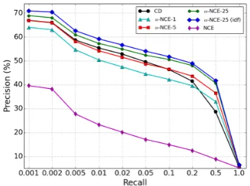
Figure 2: Precision-Recall curves for the retrieval task on the 20 Newsgroups dataset using RSMs.

For 20 Newsgroups, we trained RSMs on the training set, and reported the results on docu-ment retrieval and docudocu-ment classification. For retrieval, we treated the testing set as queries, and retrieved documents with the same labels in the training set by cosine-similarity. Precision-recall (P-R) curves and mean average precision (MAP) are two metrics we used for evaluation. For clas-sification, we trained a softmax regression on the training set, and checked the accuracy on the test-ing set. We use this dataset to show the modelltest-ing ability of RSM with different estimators.

For IMDB, the whole training set is used for learning RSMs, and an L2-regularized logistic re-gression is trained on the labeled training set. The error rate of sentiment classification on the testing set is reported, compared with several BoW-based baselines. We use this dataset to show the general modelling ability of RSM compared with others.

We trained bothα-NCE and CD, and naturally NCE (without UCE) at a fixed vocabulary size (2000 for 20 Newsgroups, and 5000 for IMDB). Posteriors of the hidden units were used as topic features. Forα-NCE , we fixed noise level at0.5

for 20 Newsgroups and0.3for IMDB. In compar-ison, we trained CD from 1 up to 5 Gibbs steps.

perfor-(a) MAP for document retrieval (b) Document classification accuracy (c) Sentiment classification accuracy

Figure 3: Tracking the modelling performance with variantαusingα-NCE to learn RSMs. CD is also reported as the baseline. (a) (b) are performed on 20 Newsgroups, and (c) is performed on IMDB.

mance, andα-NCE greatly outperforms CD on re-trieval tasks especially around large recall values. The classification results ofα-NCE is also compa-rable or slightly better than CD. Simultaneously, it is gratifying to find that the idf-weighting in-puts achieve the best results both in retrieval and classification tasks, as idf-weighting is known to extract information better than word count. In ad-dition, naturally NCE performs poorly compared to others in Figure 2, indicating variant document lengths actually bias the learning greatly.

CD _{k=1 k=5} α-NCE_{k=25 k=25 (idf)} 64.1% 61.8% 63.6% 64.8% 65.6%

Table 1: Comparison of classification accuracy on the 20 Newsgroups dataset using RSMs.

Models Accuracy

Bag of Words (BoW) (Maas and Ng, 2010) 86.75% LDA (Maas et al., 2011) 67.42% LSA (Maas et al., 2011) 83.96% Maas et al. (2011)’s “full” model 87.44% WRRBM (Dahl et al., 2012) 87.42%

RSM:CD 86.22%

RSM:α-NCE-5 87.09%

RSM:α-NCE-5 (idf) 87.81%

Table 2: The performance of sentiment classifica-tion accuracy on the IMDB dataset using RSMs compared to other BoW-based approaches.

On the other hand, Table 2 shows the perfor-mance of RSM in sentiment classification, where model combinations reported in previous efforts are not considered. It is clear thatα-NCE learns RSM better than CD, and outperforms BoW and other BoW-based models4 _{such as LDA. Theidf}

-4_{Accurately, WRRBM uses “bag ofn-grams” assumption.}

weighting inputs also achieve the best perfor-mance. Note that RSM is also based on BoW, in-dicatingα-NCE has arguably reached the limits of learning BoW-based models. In future work, RSM can be extended to more powerful undirected topic models, by considering more syntactic informa-tion such as word-order or dependency relainforma-tion- relation-ship in representation.α-NCE can be used to learn them efficiently and achieve better performance.

4.4 Choice of Noise Level-α

In order to decide the best noise level (α) for PNS, we learned RSMs using α-NCE with different noise levels for both word count andidf-weighting inputs on the two datasets. Figure 3 shows that

α-NCE learning with partial noise (α > 0) out-performs full noise (α = 0) in most situations, and achieves better results than CD in retrieval and classification on both datasets. However, learning tends to become extremely difficult if the noise becomes too close to the data, and this explains why the performance drops rapidly whenα → 1. Furthermore, curves in Figure 3 also imply the choice of α might be problem-dependent, with larger sets like IMDB requiring relatively smaller

α. Nonetheless, a systematic strategy for choos-ing optimalα will be explored in future work. In practise, a range from0.3∼0.5is recommended.

5 Conclusions

References

Yoshua Bengio, R´ejean Ducharme, Pascal Vincent, and Christian Janvin. 2003. A neural probabilistic lan-guage model. The Journal of Machine Learning Re-search, 3:1137–1155.

James Bergstra, Olivier Breuleux, Fr´ed´eric Bastien, Pascal Lamblin, Razvan Pascanu, Guillaume Des-jardins, Joseph Turian, David Warde-Farley, and

Yoshua Bengio. 2010. Theano: a CPU and

GPU math expression compiler. In Proceedings of the Python for Scientific Computing Conference (SciPy), June. Oral Presentation.

David M Blei, Andrew Y Ng, and Michael I Jordan. 2003. Latent dirichlet allocation. the Journal of ma-chine Learning research, 3:993–1022.

George E Dahl, Ryan P Adams, and Hugo Larochelle. 2012. Training restricted boltzmann machines on word observations. arXiv preprint arXiv:1202.5695.

Yann Dauphin and Yoshua Bengio. 2013. Stochastic ratio matching of rbms for sparse high-dimensional inputs. InAdvances in Neural Information Process-ing Systems, pages 1340–1348.

Michael Gutmann and Aapo Hyv¨arinen. 2010. Noise-contrastive estimation: A new estimation princi-ple for unnormalized statistical models. In Inter-national Conference on Artificial Intelligence and Statistics, pages 297–304.

Geoffrey E Hinton and Ruslan R Salakhutdinov. 2009. Replicated softmax: an undirected topic model. In

Advances in neural information processing systems, pages 1607–1614.

Geoffrey Hinton. 2002. Training products of experts by minimizing contrastive divergence. Neural com-putation, 14(8):1771–1800.

Geoffrey Hinton. 2010. A practical guide to train-ing restricted boltzmann machines. Momentum, 9(1):926.

Thomas Hofmann. 2000. Learning the similarity of documents: An information-geometric approach to document retrieval and categorization.

Aapo Hyv¨arinen. 2007. Some extensions of score matching. Computational statistics & data analysis, 51(5):2499–2512.

Richard A Kronmal and Arthur V Peterson Jr. 1979. On the alias method for generating random variables from a discrete distribution. The American Statisti-cian, 33(4):214–218.

Andrew L Maas and Andrew Y Ng. 2010. A prob-abilistic model for semantic word vectors. InNIPS Workshop on Deep Learning and Unsupervised Fea-ture Learning.

Andrew L Maas, Raymond E Daly, Peter T Pham, Dan Huang, Andrew Y Ng, and Christopher Potts. 2011. Learning word vectors for sentiment analysis. In

Proceedings of the 49th Annual Meeting of the Asso-ciation for Computational Linguistics: Human Lan-guage Technologies-Volume 1, pages 142–150. As-sociation for Computational Linguistics.

Tomas Mikolov, Kai Chen, Greg Corrado, and Jef-frey Dean. 2013a. Efficient estimation of word representations in vector space. arXiv preprint arXiv:1301.3781.

Tomas Mikolov, Ilya Sutskever, Kai Chen, Greg S Cor-rado, and Jeff Dean. 2013b. Distributed representa-tions of words and phrases and their compositional-ity. InAdvances in Neural Information Processing Systems, pages 3111–3119.

Andriy Mnih and Geoffrey E Hinton. 2009. A scal-able hierarchical distributed language model. In

Advances in neural information processing systems, pages 1081–1088.

Andriy Mnih and Yee Whye Teh. 2012. A fast and simple algorithm for training neural probabilistic language models.arXiv preprint arXiv:1206.6426. Frederic Morin and Yoshua Bengio. 2005.

Hierarchi-cal probabilistic neural network language model. In

Proceedings of the international workshop on artifi-cial intelligence and statistics, pages 246–252. Cite-seer.

Ruslan Salakhutdinov and Geoffrey Hinton. 2009. Se-mantic hashing. International Journal of Approxi-mate Reasoning, 50(7):969–978.

Gerard Salton and Michael J McGill. 1983. Introduc-tion to modern informaIntroduc-tion retrieval.

Nitish Srivastava, Ruslan R Salakhutdinov, and Ge-offrey E Hinton. 2013. Modeling documents with deep boltzmann machines. arXiv preprint arXiv:1309.6865.