Using Boosted Regression Trees and Remotely Sensed Data to Drive Decision Making

http://www.scirp.org/journal/ojs ISSN Online: 2161-7198

ISSN Print: 2161-718X

DOI: 10.4236/ojs.2017.75061 Oct. 31, 2017 859 Open Journal of Statistics

Using Boosted Regression Trees and Remotely

Sensed Data to Drive Decision-Making

Brigitte Colin, Samuel Clifford, Paul Wu, Samuel Rathmanner, Kerrie Mengersen

School of Mathematical Sciences, Queensland University of Technology, Brisbane, Australia

Abstract

Challenges in Big Data analysis arise due to the way the data are recorded, maintained, processed and stored. We demonstrate that a hierarchical, multi-variate, statistical machine learning algorithm, namely Boosted Regression Tree (BRT) can address Big Data challenges to drive decision making. The challenge of this study is lack of interoperability since the data, a collection of GIS shapefiles, remotely sensed imagery, and aggregated and interpolated spatio-temporal information, are stored in monolithic hardware components. For the modelling process, it was necessary to create one common input file. By merging the data sources together, a structured but noisy input file, show-ing inconsistencies and redundancies, was created. Here, it is shown that BRT can process different data granularities, heterogeneous data and missingness. In particular, BRT has the advantage of dealing with missing data by default by allowing a split on whether or not a value is missing as well as what the value is. Most importantly, the BRT offers a wide range of possibilities re-garding the interpretation of results and variable selection is automatically performed by considering how frequently a variable is used to define a split in the tree. A comparison with two similar regression models (Random Forests and Least Absolute Shrinkage and Selection Operator, LASSO) shows that BRT outperforms these in this instance. BRT can also be a starting point for sophisticated hierarchical modelling in real world scenarios. For example, a single or ensemble approach of BRT could be tested with existing models in order to improve results for a wide range of data-driven decisions and appli-cations.

Keywords

Boosted Regression Trees, Remotely Sensed Data, Big Data Modelling Approach, Missing Data

How to cite this paper: Colin, B., Clifford, S., Wu, P., Rathmanner, S. and Mengersen, K. (2017) Using Boosted Regression Trees and Remotely Sensed Data to Drive Deci-sion-Making. Open Journal of Statistics, 7, 859-875.

https://doi.org/10.4236/ojs.2017.75061

Received: September 27, 2017 Accepted: October 28, 2017 Published: October 31, 2017

Copyright © 2017 by authors and Scientific Research Publishing Inc. This work is licensed under the Creative Commons Attribution International License (CC BY 4.0).

DOI: 10.4236/ojs.2017.75061 860 Open Journal of Statistics

1. Background

Data are typically stored in various ways and various formats, mostly in mono-lithic software architectures which do not allow for interoperability. Analysis of data across multiple data sources is thus difficult, since the functionality of the single data sources with respect to input and output, maintenance, data processing, error handling and user interface is all interwoven and acts as archi-tecturally separate components. In order to create a basis for analysing the data considered here, it was required to extract the datasets from their original data-bases and combine them to form a common input file for the modelling process. It was therefore inevitable that this resulted in a data file structure which showed missing data, inconsistencies, duplicates and redundancies.

A case study is presented here to examine land use data sourced from a GIS, direct observations from an agricultural company, and remotely sensed data. The data were extracted from a relational database, Excel spreadsheets, remotely sensed imagery stored as raster data, and vector data from a Geographic Infor-mation System (GIS), directly observed and measured data in real-time and in-terpolated data. By combining these data sources to form one common basis for our analysis, issues of data volume, variety and veracity were encountered. Big Data research clearly deals with issues beyond volume and belongs not only to the ongoing digital revolution, but to the scientific revolution as well. The ques-tion posed of Big Data and illustrated in the case study presented here, is wheth-er new knowledge can be extracted from various data sources that haven’t been analysed in combination before, and can thus assist in a better and more confi-dent decision making.

2. Introduction

There is an exponential increase in interest in the use of digital data to improve decision making in a range of areas such as human systems, urban environ-ments, agriculture and national security. For example, decisions in the agricul-tural domain may require information based on vegetation or land use change, estimation of crops or biomass, distribution of native or exotic species, livestock or weed assessment and so on. One source of digital data that has generated in-tense interest over the past decades is remotely sensed imagery. These data are available from a wide range of sources, ranging from satellites to drones, and have been used for a very wide range of environmental applications [1]-[8].

DOI: 10.4236/ojs.2017.75061 861 Open Journal of Statistics

the context of collaboration between statisticians at the Queensland University of Technology and a large livestock organisation in Australia. The specific aim of the project was to develop an ensemble of models to predict the carrying capaci-ty, that is, the number of animals that can be sustained on a paddock. In order to achieve this goal we utilised remote sensing data and supporting information about climate and paddock characteristics. Further, it was important to present the results in a form that is useful for the agricultural decision makers.

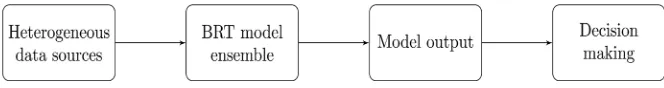
Difficult or challenging decisions demand a thorough consideration and even then they imply uncertainty, complexity and different levels of risk. Making the right decisions at the right time can lead to success, increase of profit or mini-misation of risk. It is thus important that thoughtful considerations are put into each decision. Figure 1 demonstrates the workflow following a Big Data ap-proach for our case study. Here, we use structured but heterogeneous data sources that showed characteristics like missing data, noise and redundancies. All the data sources were used to create a BRT model via an ensemble approach. The resulting model and its output serves as a foundation for a better decision making. The steps involved in the process are depicted in Figure 1. Due to commercial confidentiality concerns, the final results of the modelling workflow are not presented here.

In this article we focus on one component of the ensemble modelling ap-proach employed in the project, namely the use of BRT to estimate so-called animal equivalents per paddock. Since calves, cows and bulls of different ages consume different amounts of grass, these animals are standardised to a refer-ence animal which can then be used as a common response variable in the anal-ysis. An interesting conundrum is that one of the major inputs into such a model is the amount of grass, or more generally the biomass, in a paddock. This can potentially be estimated directly from remote sensing, but is confounded by the fact that animals are on the paddock eating the very thing that is being measured by the sensor. Moreover, the decision maker may be interested in the biomass estimates themselves, either directly via the remotely sensed measurements or indirectly via the animal equivalents based on animal weight and metabolic formula.

[image:3.595.207.539.665.709.2]

A BRT is a popular statistical and machine learning approach that has not yet seen much application in the analysis of remotely sensed data. Indeed, although they were first defined two decades ago, BRT has only recently been extended to deal with the types of features that are characteristic of remotely sensed data, in particular its spatial and temporal dynamics. Most of the activity around the use of BRT for agricultural and environmental applications does not appear in the mainstream mathematical and statistical literature.

DOI: 10.4236/ojs.2017.75061 862 Open Journal of Statistics

2.1. Case Study

The study area is located in the Northern Territory, Australia. The main climate zone is identified as grassland with hot dry summers and mild winters [9]. It is a heterogeneous region with a complex topography and land cover and type of grassland. Identification, differentiation and quantitative estimation of biomass is of primary interest in this case study. A range of data from different sources was required for this problem. In this section, we describe the information de-rived from Landsat imagery and comment briefly on other data. The reflectance recorded by the Landsat sensor is stored as an 8 bit value, resulting in a scale of 256 different grey values ranging from black (0 max absorption) to white (255 max reflection). The electronically recorded data appear as an array of numbers in digital format. In addition to the 8 bit quantisation, Landsat offers several spectral bands in the electromagnetic and infrared spectrum in which each indi-vidual pixel shows different values across different bands. This means that each pixel has a different dimension and therefore will be represented differently in each spectral band. Raster data are becoming increasingly common and increa-singly large in volume, although it is possible to reduce file size with compres-sion functions.

There is a strong advantage in using remotely sensed Landsat imagery and applied spectroscopy for these types of analyses because the data are freely available, the imagery covers a wide geographical range, and it avoids expensive, extensive and often impractical in-situ measurement. However, the trade-off is in resolution: in-situ measurements provide highly localised accuracy whereas a pixel in a Landsat image covers an area of 30 × _{30 meters. It is noted that other}

satellites are now able to provide higher resolution, but these are not yet freely available for the areas of interest in this case study.

Estimation of biomass using satellite data is of ongoing global interest. Grass biomass estimation is challenging since the phenological growing cycle of natu-rally existing grass is a dynamic process influenced by many complex parame-ters, including grass type, soil, climate, topography and land use. With the spec-tral information of remotely sensed imagery it is possible to detect green vegeta-tion, which is driven by the photosynthetic biochemical process of grass bio-mass. However, since raster imagery is only a two dimensional representation of the land cover it is difficult to derive the quantity of the vertical grass biomass directly.

vege-DOI: 10.4236/ojs.2017.75061 863 Open Journal of Statistics

tation (includes branches, dry grass, and dead leaf litter) and bare surface cover (bare soil or rocks) [11].

In addition to fractional cover Vegetation Indices (VI) are commonly used to extract meaningful information out of the imagery through image analysis tech-niques. To calculate VIs it is common to apply arithmetical methods in order to create additional artificial channels using existing spectral bands of the imagery. Other related data were also available to support the analyses. For example, SILO (Scientific Information for Land Owners) is a database of historical climate records for Australia. SILO provides daily datasets for a range of climate va-riables and in formats suitable for a variety of applications. In addition, SILO datasets are constructed from observational records provided by the Bureau of Meteorology (BOM). As another example, the AussieGRASS spatial framework includes inputs of key climate variables (rainfall, evaporation, temperature, va-pour pressure and solar radiation), soil and pasture types, tree and shrub cover, domestic livestock and other herbivore numbers. The derived results of Aussie-GRASS data are spatially interpolated to construct gridded datasets on a regular grid (approximately 5 × _{5 km) across Australia [12] [13].}

2.2. Data-Related Challenges

The analysis of relationships in ecological data sets is not trivial [14]. In addition to the complexity of the processes being modelled, there is the challenge of deal-ing with data dimensionality since it is often necessary to combine various data sources. Moreover, the scale of spatial data needs to be considered when there are differing granularities of spatial and temporal data. For example, SILO rain-fall data are reported at a 5 × _{5 km grid, whereas a Landsat pixel covers an area}

of 30 × _{30 meter. The SILO data are stored in a tabular data base format and the}

single measurement points to record the precipitation independently from each other. In contrast, the derived VI cover a whole Landsat scene of 185 × _{185 km}

and are highly correlated. All our environmental data have been provided from the Department of Science, Information Technology and Innovation (DSITI). In addition to the environmental data we used operational data provided by a commercial entity under a confidential agreement.

Another challenging characteristic of remotely sensed data is missing infor-mation. There are two major considerations in dealing with this issue. The first is dealing with the missing values. Common options are to filter them out [15] [16], interpolate them or increase the spatial aggregation. There are advantages and disadvantages to each of these approaches in terms of computational re-sources, inferential capability, and precision and bias of the resultant estimates

[17]. The second consideration is whether to undertake the chosen method as part of the pre-processing or post-processing steps.

DOI: 10.4236/ojs.2017.75061 864 Open Journal of Statistics

of working with single pixel values we reduced the volume of data by deriving descriptive statistics from Landsat, MODIS and SILO data, thereby obtaining paddock specific means, medians, first quartile, third quartile, variance and Shannon Entropy. With respect to our response variable, we aggregated real- time measurements to a monthly mean. In the next step we created a test and a training data set by partitioning the data to 20% and 80% respectively. The training set was used to estimate the model parameters. The test set was used for model performance evaluation on unseen data.

3. Boosted Regression Trees

Boosted Regression Trees (BRT), also known as Gradient Boosted Machine (GBM) or Stochastic Gradient Boosting (SGB), are non-parametric regression techniques that combine a regression tree with a boosting algorithm [18]. This extension to the classical regression tree allows greater flexibility and predictive performance in modelling the data. The implementation of these methods used in this study can be found in the gbm R package.

A regression tree partitions the data with a hierarchy of binary splits that de-fine regions of the covariate space in which the response variable has similar values. These splits are defined by rules, distance metrics or information gain. The choice of variables and the value at which the split point occurs is deter-mined in a recursive manner at each stage of the tree construction. The segmen-tation can be depicted as a tree-like structure, comprising nodes representing the selected factors, branches acting as if-else connectors between the nodes, and leaves representing terminal nodes containing the subsets of responses [19] [16] [20].

Boosting improves the performance of a simple base-learner by reweighting observations that were misclassified or had large residual errors in the previous iteration. The deeper we grow the tree, the more segments we can accommodate and thus more variance can be explained. This results in higher model complex-ity and therefore higher risk of overfitting the model to the data.

The motivation behind Boosting is that each tree can be quite shallow (a weak classifier) and thus fast to estimate, but by combining the predictive power of many weak classifiers, a classifier of arbitrary accuracy and precision can be created [21] [22] [23].

Gradient Boosting

In this section we give a brief summary of the method, following Friedman [18]. This supervised machine learning approach deals with a response variables y and a vector of predictor variables x that are connected via a joint probability

dis-tribution P

(

x,y

)

. Using a training sample

{

(

x₁,y₁

)

,,

(

xn,yn

)

}

of known

values of x and corresponding values of y, the goal is to find an approximation

( )

F x to a function *

( )

F x that minimises the expected value of a loss

DOI: 10.4236/ojs.2017.75061 865 Open Journal of Statistics

( )

( )

(

( )

)

*

,

arg min _y , .

F

F = E _xψ y F

x

x x (1)

Boosting approximates *

( )

F x by an “additive” expansion in the form of

( )

(

)

0 ; , M m m m

F

β

h

=

∑

x x a (2)

where the functions h x a

(

;

)

are generally simple functions of x with

para-meters a=

{

a a1, 2,

}

. The parameters

{ }

0 M m

a and the expansion coefficients

{ }

0 M m

β are jointly fit to the training data. This is done in a forward stage wise manner. Gradient Boosting [18] approximately solves differentiable loss func-tions ψ

(

y F,

( )

x

)

with a two step procedure. First, the function h x a

(

;

)

is fit

by least squares to the current “pseudo”-residuals

( )

(

)

( )

_{( ) ( )} 1 , m i i im i F F y F y F ψ − = ∂  = −   ∂      x x x

x (3)

which represent the residuals from the given stage of the tree building.

Then, given h x a

(

; _m

)

, the optimal value of the coefficient β_m is calculated

via

( )

(

)

(

1

)

1

arg min , ; .

N

m i m i i m

i

y F h

β

β

ψ

−

β

=

=

∑

x + x a (4)

Gradient Tree Boosting performs this with a base learner h x a

(

;

)

of an L

terminal node regression tree. A regression tree partitions the feature space into

L disjoint regions

{ }

1 L lm l

R ₋ and predicts a separate constant value at each

itera-tion m.

{ }

(

)

₁

(

)

1

; 1 .

L L

lm lm lm

l

h R y R

−

=

∑

∈

x x

(5)

The parameters of the base learner are the splitting variables and correspond-ing split points that define the tree, and this defines the correspondcorrespond-ing regions

{ }

₁L lm

R of the partition at each iteration. These are accomplished in a top-down

“best-first” approach using a least squares splitting measure [18]. Equation 4 can be solved individually within each region Rlm defined by the corresponding

terminal node l of the mth tree. Because the tree in Equation (5) predicts a

constant value ylm within each region Rlm, the solution to 4 reduces to a

sim-ple location estimate based on the criterion

ψ

( )

(

1

)

arg min , .

i lm

lm i m i

R

y F

γ

γ

ψ

−

γ

∈

=

∑

+

x

x (6)

Next, the current approximation Fm−1

( )

x is individually updated in all of

the corresponding regions

( )

1

( )

1

(

)

.

m m lm lm

F x =F ₋ x + ⋅ν γ x∈R (7)

DOI: 10.4236/ojs.2017.75061 866 Open Journal of Statistics

replacement. This subsample is then used to fit the base learner and compute the model update for the current iteration. By adding randomness to the algorithm the performance of gradient boosting was improved and this resulted in the sto-chastic Gradient Boosting Machine (GBM) [23]. The Stochastic Gradient Boost-ing algorithm is summarised as pseudo code below [15] [23]. The input training data is defined through

{

_i, _i

}

N

i

y x and

{ }

( )

N

i

i

π is the random permutation of the integers 1,,N . The random subsample of size N<N is given by

( ) ( )

{

,

}

1

N

i i

y_{π π}



x .

4. Results

The data were presented as a set

{

(

x yi, i

)

0≤ <i nsamples

}

with feature vector features

n i∈

x  , and the response y_i∈. All the data we used for our case study

DOI: 10.4236/ojs.2017.75061 867 Open Journal of Statistics

test data, resulting in 167 training and 42 test observations.

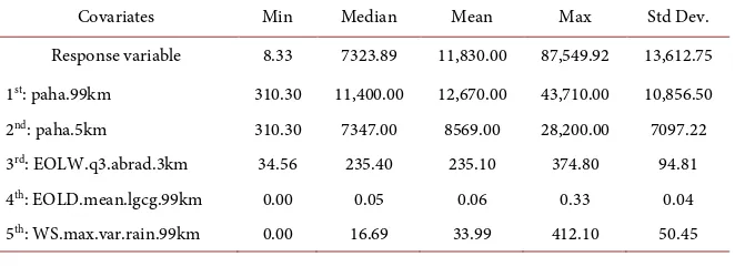
The computational environment was the R statistical modelling software ver-sion 3.3.3 [24] running inside Windows 7 SP1 (64-bit) on a 2.60 GHz Intel i7 CPU with 16 GB of RAM. All of the results and illustrations were created in the R programming language. The GBM model implementations for this article were taken from the gbm packages. Table 1 show the distribution of the re-sponse variable and the most influential covariates. Please see Figure 3 as a fur-ther reference in regards of their individual contribution in the splitting process. One way of showing the complex relationships of the joint probability and contribution of each covariate in describing the response is through a relative in-fluence plot. Relative inin-fluence measures are calculated by averaging the number of times a covariate is used for splitting, weighted by the squared improvement to the model as the result of each split. It is then scaled so the values sum to 100.

In Figure 2 we present a relative influence plot for all of the available va-riables. The relative influence of the 141 variables varies considerably, with some never contributing (0%) and only 20 variables having relative influence greater than 2.9% as depicted in Figure 3. The two variables that contribute the most are paha.99km at 10.8%, followed by paha.5km with 9.56%. The third strongest variable is EOLW.q3.abrad.3km which contributes with only %3.83. Figure 3

shows the top five contributors on a log scale plot.

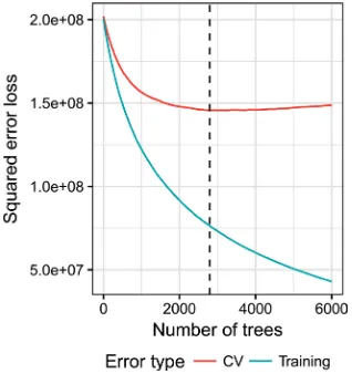
Regularisation methods are used to constrain the fitting procedure so that it balances model fit and predictive performance [15]. Regularisation is particular-ly important for BRT because its sequential model fitting allows trees to be add-ed until the data are completely overfittadd-ed [25]. As discussed in section 3, intro-ducing some randomness into a boosted model usually improves accuracy and speed and reduces overfitting [23].

[image:9.595.210.541.609.734.2]

Figure 4 describes the effect of regularisation on the squared error loss. The blue line is the error in the training data, the red line in the test data. The vertical dashed line indicates the optimal number of iterations/trees provided by the gbm model where the test data reaches its minimum, here at 2784 trees. After reaching the minimum, the graph of the squared error loss starts to increase again. This change of direction indicates the start of the model overfitting the training data and therefore poorly explaining the variation seen in the test data.

Table 1. Distribution of the response variable and key predictors. Predictor names are described in text.

Covariates Min Median Mean Max Std Dev. Response variable 8.33 7323.89 11,830.00 87,549.92 13,612.75 1st_{: paha.99km 310.30 11,400.00 12,670.00 43,710.00 10,856.50}

2nd_{: paha.5km 310.30 7347.00 8569.00 28,200.00 7097.22}

3rd_{: EOLW.q3.abrad.3km 34.56 235.40 235.10 374.80 94.81}

4th_{: EOLD.mean.lgcg.99km 0.00 0.05 0.06 0.33 0.04}

[image:10.595.190.539.56.242.2]

DOI: 10.4236/ojs.2017.75061 868 Open Journal of Statistics

Figure 2. Relative influence plots of all 141 covariates showing their contribution in the split-ting process. The horizontal axis indicates the frequency of the contribution with the maxi-mum of 10.8%.

Figure 3. Subset of a relative influence plots of covariates with a contribution greater than 2.9% (log scale).

[image:10.595.188.540.294.466.2] [image:10.595.285.444.514.683.2]

DOI: 10.4236/ojs.2017.75061 869 Open Journal of Statistics

The bias-variance trade-off goal is to find the optimal number of trees where the bias and the variance are balanced and the error is minimised, since both under- and overfitting will have a negative effect on the predictive performance of the model.

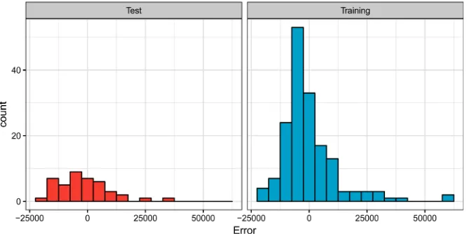
[image:11.595.209.542.441.608.2]

Histograms of the residuals for the test and training sets are shown in Figure 5. In comparison to the training data the test data does not have multiple peaks—which often indicate that important variables are not yet accounted for— but there are some large positive outliers in the training data, beyond 50,000.

Table 2 shows the results of the comparison of BRT and other methods. It is

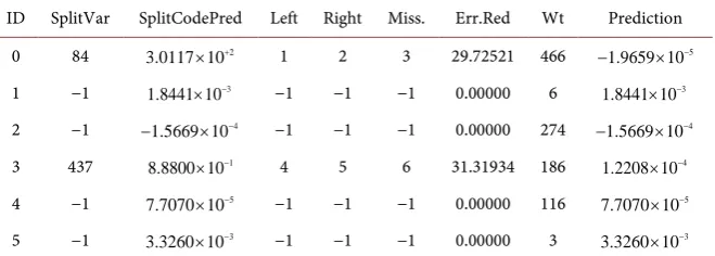
seen that the BRT performed best in fitting the data according to the RMSE. One of the biggest advantages in using a BRT is that it can handle missing values in the predictors by default. As part of the model diagnostics, we can plot how the data have been split, to which node they have been assigned, and the reduction in error for this single iteration/tree. If the tree is challenged with data that are missing a variable, the split is decided based on a surrogate variable, typically one that has a high correlation with non-missing observations.

The R function pretty.gbm.tree() returns a data frame in which each row cor-responds to a node in the tree (Table 3). Here, the root node (indicated by the row number 0) is split by the 84th _{SplitVar (splitting variable). Since the}

num-bering starts with 0 the split variable is the 85th _{column in the training set of our}

case study. Rows in the table with a SplitVar of −1 are terminal nodes. A Split-CodePred value of 301.171 denotes that all points less than 301.17 were allocated to the left node 1 (and hence all points greater then 301.17 were allocated to the right node 2). All points that had a missing value in this column were assigned

[image:11.595.208.538.656.729.2]

Figure 5. Histogram of residuals in the test and training sets at the optimal tree size.

Table 2. Overall model average prediction performance, based on 500 cross-validations.

Method RMSE

Random Forest BRT LASSO

[image:12.595.210.540.90.208.2]

DOI: 10.4236/ojs.2017.75061 870 Open Journal of Statistics

Table 3. Summary of gbm single tree prediction in pretty.gbm.tree.

ID SplitVar SplitCodePred Left Right Miss. Err.Red Wt Prediction 0 84 _{3.0117 10×} +2 _{1 2 3 29.72521 466 −1.9659 10×} −5

1 −1 3

1.8441 10× − −1 −1 −1 0.00000 6 3 1.8441 10× −

2 −1 _{−1.5669 10×} −4 _{−1 −1 −1 0.00000 274 −1.5669 10×} −4

3 437 1

8.8800 10× − 4 5 6 31.31934 186 4 1.2208 10× −

4 −1 _{7.7070 10×} −5 _{−1 −1 −1 0.00000 116 7.7070 10×} −5

5 −1 3

3.3260 10× − −1 −1 −1 0.00000 3 3 3.3260 10× −

to the missing node 3. If the node is a terminal node then this is the prediction. The error reduction (29.73) indicates the reduction in the loss function as a re-sult of splitting this node and there were 466 weights (weights will be on each node) in the root node. The weight indicates the total weight of observations in the node. The last column prediction of −0.000019659 denotes the value as-signed to all values at this node before the point was split. The prediction col-umn refers to individual trees and they are fit to predict the gradient of the loss function evaluated in the current prediction and the response. This is the gra-dient part of Gragra-dient Boosting.

5. Discussion

In this case study we demonstrated that BRT is able to address Big Data chal-lenges, produce satisfying results and can deal with missing values by default. In addition, we obtained in-depth knowledge of the diverse and heterogeneous data sources used in this study, and identified key covariates that were most influen-tial in describing the response variable. Further, descriptive statistics has been used to quantitatively describe our data and basic features of it by providing summaries that enables us to present our results in a meaningful way and there-fore allowed for a simpler interpretation. The histograms of training and test data showed us the underlying frequency distribution of our continuous data. In this case both histograms are left skewed and demonstrate that the majority of data can be found on the left hand side. Because histograms use bins to display data it is not possible to see exactly what the specific values are for the minimum and maximum. However, we can see an approximation of the range of values, see how spread out the data are and that there are not outliers that we need to take care of. One of the biggest disadvantages of BRT is, that they are prone to overfit the data, thus appropriate settings for the hyperparameters need to be set in order to control the model building process. It is therefore advisable to tune the model hyperparameters as part of a pre-processing step in an iterative man-ner prior to performing the final modelling.

accom-DOI: 10.4236/ojs.2017.75061 871 Open Journal of Statistics

modate missing data, include different types of input variables without the need for transformations, perform well in high-dimensional problems, and allow for different loss functions such as accurate identification of small areas of interest. Moreover, they can be visualised and interpreted easily, thus facilitating the translation of the analytic results to decision makers [18]. BRT have also been compared favourably with other flexible regression approaches such as genera-lised additive models [14]. An example of BRT models helping in developing an understanding of missingness structure in the data is given by [26]. In this study Tierney [26] concluded that more knowledge was gained about the origins of the data and the data collection process, as well as the handling of missing values for future analysis. In another study [26], the author took a different approach to deal with missing values by taking summary values such as the mean over grouped data.

There are several challenges in using BRT for this case study. First, the volume of one single satellite imagery is quite high even without aggregating or com-bining them in a dense time series. One Landsat satellite scene covers 185 × ₁₈₅

km of land and has a file size of about 300 MB. The temporal resolution of Landsat is on average 16 days; thus, in one year there are 22 scenes of the same area to computationally process, analyse and store, a data volume of about 6.6 GB. Examination of several years of satellite imagery yields in enormous geo-temporal datasets. Given these specifications, a substantive challenge is the storage, processing and management of massive volumes of raster data informa-tion. This challenge is exacerbated when the other input variables are also con-sidered, especially since these are of different data formats, sources, structure and spatial granularities. In order to decrease the volume we calculated descrip-tive statistics based on individual paddock information instead of using pixel in-formation for our analysis.

The second challenge is determining the geographic area to include in the sta-tistical models. The region of interest is spread over multiple stations, with mul-tiple paddocks per station. However, not all of the land in a paddock is grazable. Jansen [27] investigated the quantification of livestock effects on the scalable, season specific metric of Landsat imagery and biomass identification and devel-opment of a model assessing spatial relationships between spectral indices and ruminants over a growing season. The focus was on finding significant correla-tions between existing biomass, vegetation metrics and management practices to quantify changes in vegetation due to grazing. Changes can be caused not only through overgrazing and loss but also due to changes in phenology caused by climate variability and also availability of water. The spatial distribution of ani-mal impacts becomes organised along an utilisation gradient termed a piosphere

availa-DOI: 10.4236/ojs.2017.75061 872 Open Journal of Statistics

ble foraging area. In addition to the concentric rings there are also natural water streams which attract the animals and provide biomass along those linear fea-tures. So-called linear buffer zones can be calculated along the streams to indi-cate grazing areas nearby the water, like the concentric rings around the water points. The quantity and quality of biomass types can be extracted through the spectral values of the Landsat pixels and with additional spatial data, in particu-lar fractional cover which identifies three categories of ground cover percentage (photosynthetic vegetation, non-photosynthetic vegetation and bare soil).

The third challenge is incorporating spatial information with disjoint geo-graphic areas (agricultural properties or stations), each of which comprises re-gions (paddocks) of varying sizes. In the case study, the provided information was typically in the form of summary values per paddock per month. Seasonal (wet and dry) indicators were also used to help quantify the biomass [29] and define the spatial extent of the area due to varying rainfall. The beginning of the dry season is a critical time stamp in terms of predicting the amount of grass that will be available during the dry season and the corresponding decision re-garding the number of animals to be placed in paddocks to avoid the negative impact of over- or under grazing.

There is a large literature on the predictive, methodological and computation-al properties of decision trees, including the Random Forest (RF) and Boosted Regression Tree (BRT) models used in this paper. The predictive accuracy of these methods has been investigated both theoretically [30] [31] [32] [33] and in various applications [34]. The latter authors also compared modelling ap-proaches considered in this paper in the analysis of a large epidemiological da-taset and concluded that RF, BRT and LASSO outperformed the conventional logistic regression framework. Methodologically, decision tree approaches be-long to the family of greedy algorithms and select variables in a forward selec-tion manner. Both of these features strongly influence the convergence speed and computational time [18] [23]. The computational time is also influenced by the choice of model parameters such as the learning rate and tree complexity

[25]. For example, while a smaller shrinkage parameter slows down the learning rate and results in better predictive performance, the trade-off is a larger number of iterations in order to converge to a local minimum and therefore a longer computational time. The total running time also depends on the choice of loss function, regularisation method and the measure of convergence [31]. Empirical comparisons of the running time of different tree methods such as RF and BRT have also been published [35].

DOI: 10.4236/ojs.2017.75061 873 Open Journal of Statistics

big, noisy and spatial data is the Bayesian additive regression model [36], a Bayesian sum-of-tree model that generates samples from a posterior. Further, a sum-of-trees model is an additive model with multivariate components. Com-pared to generalized additive models based on sums of low dimensional smoothers [37] [38], these multivariate components can more naturally incor-porate interaction effects. This approach enables full posterior inference includ-ing point and interval estimates of the unknown regression function as well as the marginal effects of potential predictors. Gathering large and diverse envi-ronmental data is essential in this field and analysing those covariates is chal-lenging. Big data has notable effects on predictive analytic, knowledge extraction and interpretation tools [39] and appropriate methods need to be applied in or-der to gain new knowledge of data-driven discoveries that assist in decision making.

Acknowledgements

This research was undertaken through the Australian Cooperative Research Centre for Spatial Information with the Project number P4.101. We thank our colleagues for their insight and expertise, particularly Dr. Michael Schmidt (De-partment of Science, Information Technology and Innovation) for providing key publications of the Wambiana Grazing Trial and helpful discussions.

References

[1] Schmidt, M., Thamm, H.P. and Menz, G. (2003) Long Term Vegetation Change Detection in an Arid Environment Using Landsat Data. Geoinformation for Euro-pean-Wide Integration, Millpress, Rotterdam.

[2] Marsett, R.C., Qi, J., Heilman, P., Biedenbender, S., Watson, M.C., Amer, S., Weltz, M., Goodrich, D. and Marsett, R.C. (2006) Remote Sensing for Grassland Manage-ment in the Arid Southwest. Rangeland Ecology & Management, 59, 530-540. https://doi.org/10.2111/05-201R.1

[3] Huete, A., Ponce-Campos, G., Zhang, Y., Restrepo-Coupe, N., Ma, X. and Moran, M.S. (2015) Land Resources Monitoring, Modeling, and Mapping with Remote Sensing, Monitoring Photosynthesis from Space, CRC Press.

[4] Jafari, A., Khademi, H., Finke, P.A., Van de Wauw, J. and Ayoubi, S. (2014) Spatial Prediction of Soil Great Groups by Boosted Regression Trees Using a Limited Point Dataset in an Arid Region, Southeastern Iran. Geoderma, 232-234, 148-163. https://doi.org/10.1016/j.geoderma.2014.04.029

[5] Anderson, M.C., Allen, R.G., Morse, A. and Kustas, W.P. (2012) Use of Landsat Thermal Imagery in Monitoring Evapotranspiration and Managing Water Re-sources. Remote Sensing of Environment, 122, 50-65.

https://doi.org/10.1016/j.rse.2011.08.025

[6] Washington-Allen, R.A., Van Niel, T.G., Ramsey, R.D. and West, N.E. (2004) Re-mote Sensing Based Piosphere Analysis. GIScience and Remote Sensing, 41, 136-154. https://doi.org/10.2747/1548-1603.41.2.136

DOI: 10.4236/ojs.2017.75061 874 Open Journal of Statistics [8] Sarker, C., Mejias Alvarez, L. and Woodley, A. (2016) Integrating Recursive Baye-sian Estimation with Support Vector Machine to Map Probability of Flooding from Multispectral Landsat Data. International Conference on Digital Image Computing:

Techniques and Applications. https://doi.org/10.1109/DICTA.2016.7797054 [9] Australian Bureau of Meteorology (2016) Climate classification of Australia,

http://www.bom.gov.au/climate/averages/climatology/gridded-data-info/metadata/ md_koppen_classification.shtml

[10] Scarth, P. (2017) Fractional Cover—Landsat, Joint Remote Sensing Research Pro-gram Algorithm, Australia Coverage.

http://data.auscover.org.au/xwiki/bin/view/Product+pages/Landsat+Fractional+Co ver

[11] Scarth, P.F., Röder, A. and Schmidt, M. (2010) Fractional Cover. Proceedings of the

15th Australasian Remote Sensing and Photogrammetry Conference. [12] DSITI (2015) AussieGRASS Environmental Calculator.

https://www.longpaddock.qld.gov.au/about/publications/pdf/agrass_user_guide.pdf [13] Bastin, G., Denham, R., Scarth, P., Sparrow, A. and Chewings, V. (2014) Remote-ly-Sensed Analysis of Ground-Cover Change in Queensland’s Rangelands, 1988-2005.

Rangeland Journal, 36, 191-204. https://doi.org/10.1071/RJ13127

[14] Leathwick, J.R., Elith, J., Francis, M.P., Hastie, T. and Taylor, P. (2006) Variation in Demersal Fish Species Richness in the Oceans Surrounding New Zealand: An Anal-ysis Using Boosted Regression Trees. Marine Ecology-Progress Series, 321, 267-281. https://doi.org/10.3354/meps321267

[15] Hastie, T., Tibshirani, R. and Friedman, J. (2009) The Elements of Statistical Learn-ing. Springer Series in Statistics, New York.

https://doi.org/10.1007/978-0-387-84858-7

[16] Tarling, R. (2009) Statistical Modelling for Social Researchers: Principles and Prac-tice. Taylor & Francis Group, Abingdon.

[17] De’ath, G. and Fabricius, K.E. (2000) Classification and Regression Trees: A Po-werful yet Simple Technique for Ecological Data Analysis. Ecology, 81, 3178-3192. https://doi.org/10.1890/0012-9658(2000)081[3178:CARTAP]2.0.CO;2

[18] Friedman, J.H. (2001) Greedy Function Approximation: A Gradient Boosting Ma-chine. Institute of Mathematical Statistics, 29, 1189-1232.

http://www.jstor.org/stable/2699986

[19] Robinzonov, N. (2013) Advances in Boosting of Temporal and Spatial Models. Ludwig-Maximilians-Universität München.

http://edoc.ub.uni-muenchen.de/15338/

[20] James, G. and Witten, D. and Hastie, T. and Tibshirani, R. (2013) An Introduction to Statistical Learning. Springer Texts in Statistics, Springer-Verlag, New York, 856-875. https://doi.org/10.1007/978-1-4614-7138-7

[21] Breiman, L. (1998) Arcing Classifiers. Annals of Statistics, 26, 801-849.

[22] Freund, Y. and Schapire, R.E. (1996) Experiments with a New Boosting Algorithm.

International Conference on Machine Learning, Bari, 3-6 July 1996, 148-156. http://dl.acm.org/citation.cfm?id=3091696.3091715

[23] Friedman, J.H. (2002) Stochastic Gradient Boosting. Computational Statistics and Data Analysis, 28, 367-378. https://doi.org/10.1016/S0167-9473(01)00065-2

[24] R Core Team (2017) R: A Language and Environment for Statistical Computing. https://www.R-project.org/

Regres-DOI: 10.4236/ojs.2017.75061 875 Open Journal of Statistics sion Trees. Journal of Animal Ecology, 77, 802-813.

https://doi.org/10.1111/j.1365-2656.2008.01390.x

[26] Tierney, N.J., Harden, F.A., Harden, M.J. and Mengersen, K.L. (2015) Using Deci-sion Trees to Understand Structure in Missing Data. BMJ Open, 5, 1-12.

https://doi.org/10.1136/bmjopen-2014-007450

[27] Jansen, V., Kolden, C., Taylor, R. and Newingham, B. (2016) Quantifying Livestock Effects on Bunchgrass Vegetation with Landsat ETM+ Data across a Single Growing Season. International Journal of Remote Sensing, 37, 150-175.

https://doi.org/10.1080/01431161.2015.1117681

[28] Derry, J.F. (2004) Piospheres in Semi-Arid Rangeland: Consequences of Spatially Constrained Plant-Herbivore Interactions. The University of Edinburgh, 1-305. http://hdl.handle.net/1842/600

[29] Humphries, G.R.W. (2015) Estimating Regions of Oceanographic Importance for Seabirds Using A-Spatial Data. PLoS ONE, 10, 1-15.

https://doi.org/10.1371/journal.pone.0137241

[30] Schapire, R. (2003) The Boosting Approach to Machine Learning: An Overview.

MSRI Workshop on Nonlinear Estimation and Classification, Springer, New York. https://doi.org/10.1007/978-0-387-21579-2_9

[31] Chipman, H.A., George, E.I. and McCulloch, R.E. (2001) The Elements of Statistical Learning: Data Mining, Inference and Prediction. Springer, New York.

[32] Bell, J.F. (1999) Tree-Based Methods, Machine Learning Methods for Ecological Applications. Kluer, Dordrecht, 89-105.

https://doi.org/10.1007/978-1-4615-5289-5_3

[33] Breiman, L., Friedman, J., Olshen, R. and Stone, C. (1984) Classification and Re-gression Trees. Chapman and Hall, Wadsworth, New York.

[34] Tsangaratos, P. and Ilia, I. (2016) Landslide Susceptibility Mapping Using a Mod-ified Decision Tree Classifier in the Xanthi Perfection, Greece. Landslides, 13, 305-320. https://doi.org/10.1007/s10346-015-0565-6

[35] Cormen, T.H., Leiserson, C.E., Rivest, R.L. and Stein, C. (2009) Introduction to Al-gorithms. The MIT Press, Cambridge, Massachusetts.

[36] Chipman, H.A., George, E.I. and McCulloch, R.E. (2010) BART: Bayesian Additive Regression Trees. Annals of Applied Statistics, 4, 266-298.

https://doi.org/10.1214/09-AOAS285

[37] Hastie, T.J. and Tibshirani, R. (1986) Generalized Additive Models. Statistical Science, 1, 297-310. https://doi.org/10.1214/ss/1177013604

[38] Wood, S.N. (2011) Fast Stable Restricted Maximum Likelihood and Marginal Like-lihood Estimation of Semiparametric Generalized Linear Models. Journal of the Royal Statistical Society (B), 73, 3-36.

https://doi.org/10.1111/j.1467-9868.2010.00749.x

[39] Lary, D.J., Alavi, A.H., Gandomi, A.H. and Walker, A.L. (2016) Machine Learning in Geosciences and Remote Sensing. Geoscience Frontiers, 7, 3-10.