Investigating the effect of efficiency and technical changes on productivity

Munich Personal RePEc Archive

Investigating the effect of efficiency and

technical changes on productivity

Halkos, George and Bampatsou, Christina

Department of Economics, University of Thessaly, Public Power

Corporation S.A.

December 2016

Online at

https://mpra.ub.uni-muenchen.de/76287/

1

Investigating the effect of efficiency and technical

changes on productivity

Christina Bampatsou

_{& George Halkos}

1 _{Public Power Corporation S.A. Greece}

2 _{Laboratory of Operations Research,}

Department of Economics, University of Thessaly

[email protected], [email protected]

Abstract

Better management of natural capital, an efficient allocation of resources and technological progress can contribute to productivity change. The present study uses Data Envelopment Analysis to determine the Total Factor Productivity Index, in the case of the EU15 countries, using panel data on energy consumption for a period spanning from 1995 to 2011. The aim is not only to determine the index of total factor productivity change but also to record its driving forces for the decision making units under consideration, showing whether the productivity gains come mainly from an improvement in efficiency or derive merely as a result of technological progress. In terms of eco-efficiency, the paper contributes in showing whether the overall development is more driven by input-saving or environmental-saving processes. The detailed decomposition offers policy makers additional insights into more valuable reference material representing the driving forces of productivity gains or losses.

Keywords: Energy; Energy Consumption; Environmental Economics; Carbon emissions; Eco-Efficiency; Data envelopment analysis; Total factor productivity index.

2 1. Introduction

As reported by Bampatsou et al. (2013) the higher share of renewable energy

varieties in an energy mix of a country is a necessary but not a sufficient condition for its

economic system’s sustainability. This is justified by the higher energy demand that

cannot be met by relying only on renewable sources. However, the continuation of high

energy productivity levels is necessary to guarantee the fulfilment of the energy needs of

a country (see Bampatsou et al., 2013). In this study we focus on the trend of energy

consumption in order to develop a more thoughtful measure of the aspects influencing

production efficiency under specific output conditions. Furthermore, bringing together

economic and environmental issues, the concept of economic and ecological efficiency,

known as eco-(in)efficiency, is utilized.

As indicated by Mahlberg et al. (2011) the concept of eco-efficiency claims that it

is possible to produce higher levels of goods and services causing less environmental

degradation and less consumption of natural resources. As we demonstrate further in this

study it is possible for Decision Making Units (henceforth DMUs) to be more efficient or

to increase the efficiency and maintain a certain level of environmental performance or to

improve both targets simultaneously.

The index of eco inefficiency is a quantity measure in the case of carbon dioxide,

which is not priced in most markets. The index incorporates carbon dioxide emissions as

undesirable output. Therefore, is not limited to the measurement of productive efficiency

for operations involving environmental negative externalities produced by the fossil fuel

energy production process (see among others, Chen and Delmas, 2012; Halkos and

3

The contribution of the paper is twofold: First, by adopting this approach, we are

able to identify whether the productivity increase over multiple time periods is a result of

an improvement in technical efficiency or a result of technological progress. In this

regard, we manage to highlight whether productivity change is more driven by

input-saving, environmental-saving or both. Thus, we obtain a useful insight into the way of

transforming inputs into outputs. Moreover, the productivity change that may arise from

the different composition of the total energy mixture by time is an important topic to be

considered.

Second, we apply the Data Envelopment Analysis (DEA) method at a

macroeconomic level. This allows us to investigate the performance of the economic

systems of the EU15 countries using panel data on energy consumption during

1995-2011. Under these conditions, and following the spirit of the dynamic Malmquist Total

Factor Productivity Change (TFPCH) index in the presence of undesirable output, the

productivity of energy consumption is measured in order to decompose the TFPCH into

two components representing the changes of eco-technical and eco-efficiency

respectively.

After a very brief review of the Malmquist productivity index in section 2, the

remaining of this paper is organized as follows. Section 3 presents the data set and the

empirical methodology. Section 4 contains the empirical results and section 5 discusses

the empirical findings in order to have a better understanding of the content of the

productivity change from cross-country comparisons. Finally, section 6 concludes with

4 2. The Malmquist productivity index: A brief history review

Total Factor Productivity (TFP) is a measure of production efficiency and is

defined as the index of all outputs divided by all inputs (see, among others Fischer et al.,

2009; Kitcher et al., 2013). The concept of the Total Factor Productivity index was

suggested by Malmquist (1953) and its development can be calculated using the

Malmquist index. The Malmquist index of TFP growth was developed through a general

production function framework by Caves et al. (1982).

Malmquist’s TFP index can be used to measure the TFPCH of DMUs between

two data points by estimating the ratio of distances of each data point in relation to a

common technology. The productivity change is determined by the contribution of i)

technology innovation (see Sarkis and Weinrach, 2001), ii) productivity improvement

(see Bevilacqua and Braglia, 2002), and iii) optimal allocation of resources (see Kuo et

al., 2010; Fukuyama et al., 2013).

The calculation of the TFP index can be obtained using both parametric and

non-parametric approaches (see Fried et al., 2008). In parametric approaches, the distance

functions are determined by parametric methods and, for this reason, the production

frontier is a stochastic frontier. In non-parametric approaches, like the one utilized in the

present study, the Malmquist Index can be obtained through DEA. The most popular

non-parametric approaches used for calculating the distance functions are the linear

programming models developed by Färe et al., (1994b).

The relevant literature has used the DEA based Malmquist Productivity Index to

calculate the performance of different DMUs over time, in the presence of undesirable

5

2015; Long et al., 2015). More recently, Makridou et al. (2015) suggest an overall energy

efficiency and composite performance indicator combining DEA and Multiple Criteria

Decision Aiding Methodology (MCDA). Wang and Wei (2016) utilize the Luenberger

productivity index, which is also used to calculate productivity change and its

components, to analyze energy input-specific and environmental productivity change in

China.

As indicated by Murillo-Zamorano (2005) the consideration of technical

efficiency contributes to a better understanding of both the temporal evolution and

cross-country variability of aggregated productivity growth. However, the research on the

driving forces of productivity gains or losses in energy sector and in terms of energy

efficiency and CO2 emission performance appears very limited at microeconomic level

with more representative contribution from Martínez (2013). To the best of our

knowledge there is no research addressing the issue at macroeconomic level using the

input-specific Malmquist productivity index. Therefore, the present paper aims to fill in

this gap in order to help DMUs to evaluate economic policies more effectively.

Moreover, the current research aims to assist policymakers in improving the

eco-efficiency of economic growth with less resource consumption and lower pollution

through new technologies and more effective management of energy resources.

3. Data and methodology

DEA is used here to determine the TFP (Malmquist) Index. For this purpose panel

data on energy consumption of the EU151 countries are utilized. The time period spans

from 1995 to 2011 (i.e. T=15; N=17). To determine the Malmquist index, the entire

EU15 is considered as a separate entity and each of the individual EU15 countries is

6

taken as different DMU. Estimates are based on an input oriented DEA model.The index

of the Total Primary Energy Consumption per capita is used as input2_{, while GDP per}

capita and CO2 emissions per capita from the consumption of energy are used as

desirable and undesirable outputs respectively.

A necessary point concerning the choice of inputs and outputs is that they are not

specified following the restrictions of the traditional DEA (Halkos and Salamouris,

2004). In the context of the current application, GDP and CO2 emissions3 are not the

outputs solely due to fossil and non-fossil energy consumption but the representative

outputs and inputs relevant to the calculation of the DEA-based Malmquist productivity

index. Compared to other methods and as noted by Fagerberg (1994), TFP evaluates the

contribution of technology progress and economies of scale to economic growth without

the effect of land, capital, labor and other traditional elements. An analogous

macroeconomic context of DEA applications (cross section/panel data analysis) has been

described in the literature (see, among others, Golany and Thore, 1997; Ramanathan,

2006; Bampatsou and Hadjiconstantinou, 2009; Bampatsou et al., 2013; Xishuang et al.,

2014; Sheng et al., 2015). More recently, Sueyoshi, and Yuan, (2016), suggest a new

approach on energy and sustainability as they measure the degree on Marginal Rate of

Transformation and Marginal Rate of Substitution through DEA environmental

assessment.

2 _{Although a production function requires the use of L and K our intention is to see the direct effect of}

energy on both desirable and undesirable outputs.

3 _{For more information on CO}

2 and in general GHG emissions and the associated problems see among

7

3.1. Data sources and Definitions

For each country, the total primary energy consumption indicates the energy that

has not been subjected to any conversion or transformation process. Total primary energy

consumption includes the consumption of petroleum, dry natural gas, coal, and net

nuclear, hydroelectric and non-hydroelectric renewable electricity. It also includes net

electricity imports (imports minus exports).

CO2 emissions from the consumption of energy include emissions due to the

consumption of petroleum, natural gas, and coal, and also from natural gas flaring. Our

study focuses on CO2 because is by far the largest contributor to the greenhouse effect.

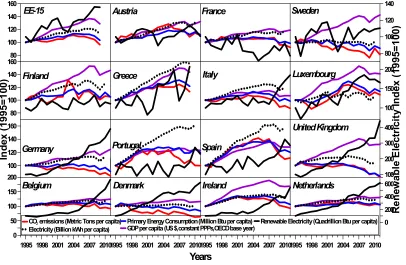
The data set is presented in a summarized form in Figure 1. All energy data comes

from EIA (2013) while all GDP data comes from OECD (2013). The left-hand side

vertical axis represents CO2 emissions, Total Primary Energy Consumption, GDP and

Electricity Net Consumption while the right-hand side vertical axis represents Renewable

Electricity Net Consumption (all expressed per capita).

As input we use the total energy consumption, composed of renewable and

exhaustible energy resources. The input is in this case responsible for the simultaneous

production of both desirable product (GDP), which typically has a positive price, and non

marketed undesirable byproduct (CO2 emissions). The fact that desirable and undesirable

outputs are jointly produced or null-jointly produced indicates, in the terminology of

Shephard and Färe (1974), that the production of desirable outputs is not possible without

8 Figure 1: Development trends of inputs and outputs for the entire EU15 and for each of

the individual EU15 countries (EIA, 2013; OECD, 2013)

1995 1998 2001 2004 2007 2010

Years 0 50 100 150 200 In de x (1 99 5= 10 0) 100 120 140 160 80 100 120 140 160

1995 1998 2001 2004 2007 20101995 1998 2001 2004 2007 20101995 1998 2001 2004 2007 2010 80 100 120 140 160 80 100 120 140 100 150 200 100 200 300 400 0 200 400 600 R en ew ab le E le ct ric ity In de x (1 99 5= 10 0)

CO2 emissions (Metric Tons percapita)

Electricity(Billion kWh percapita) Primary EnergyConsumption(Million Btu per capita)GDPpercapita(US$,constantPPPs,OECDbaseyear) RenewableElectricity (Quadrillion Btu per capita)

EE-15 Austria France Sweden

Finland Greece Italy Luxembourg

Germany Portugal Spain

United Kingdom

Belgium Denmark Ireland Netherlands

The use of the Malmquist input-oriented productivity index (TFPCH) makes

possible to decompose the productivity changes into technical change index (TECHCH)

and technical efficiency change index (EFFCH). These two indexes indicate which

factors drive the change of energy efficiency and the magnitude of this change.

3.2 The model

Following Färe et al. (1994a), the input oriented Malmquist productivity change

index may be formulated as shown in [1] for an assessment involving inputs and outputs:

2 / 1 1 1 1 1 1 1 1 1 1 ) , ( ) , ( ) , ( ) , ( ) , , , (           _      t t t I t t t I t t t I t t t I t t t t t

I y x y x D_Dy_{y x}x D_D y_y x_x

9

where I indicates an input-orientation, y denotes output, x denotes input, M is the

productivity of the most recent production point relative to the earlier production point,

and D denotes the input distance function.

The first ratio inside the brackets stands for the Malmquist index for period t. It

shows the previous production point (xt_{, y}t_{), using period t technology. It calculates}

productivity change from period t to period t+1 using the technology level at period t as a

benchmark. With the input Malmquist Productivity Index relying on technology of period

t we have:

) , (

) ,

( 1 1

t t t I t t t I t

I D_Dy_{y x}x

M    (2)

Similarly, the second ratio inside the brackets corresponds to the Malmquist index

for period t+1. It specifies the most recent production point (xt+1_{, y}t+1_{) using period t+1}

technology. It computes the change in productivity from period t to period t+1 using the

technology level at period t+1 as a benchmark. With input Malmquist Productivity Index

being based on the technology of period t+1 we have:

) , ( ) , ( 1 1 1 1 1 t t t I t t t I t

I D_D y_{y x}x

M  _ _   ₍₃₎

We may also present the Malmquist Productivity Index in a similar form as shown in [4].

2 / 1 1 1 1 1 1 1 1 1 1 1 1 1 ) , ( ) , ( ) , ( ) , ( ) , ( ) , ( ) , , , (            _ _ _{ }    t t t I t t t I t t t I t t t I t t t I t t t I t t t t t

I y x y x D_D y_{y x}x _DD y_y x_{x D}D y_y x_x

M (4) or 2 / 1 1 1 1 1 1 1 1 1 1 1 1 1 ) , ( ) , ( ) , ( ) , ( ) , ( ) , ( ) , , , ( _           _ _ _{ }    t t t I t t t I t t t I t t t I t t t I t t t I t t t t t

I y x y x D_D y_{y x}x _DD y_y x_{x D}D y_y x_x

M (5)

10

The ratio outside the brackets in equation [5] is defined as the technical efficiency

change index (EFFCH) and the ratios inside the brackets as the technical change index

(TECHCH). Therefore, the Malmquist total factor productivity index is the product of an

efficiency change over the same period and a measure of technical progress as calculated

by shifts in the frontier measured at periods t + 1 and t.

The Malmquist Index values and its components may be greater, equal or

smaller than 1. Hence, it is easy to understand that we have the following three cases:

(i) If Malmqusit Productivity Index between time periods t and t+1 is greater

than 1, then there is an improvement in energy consumption performance

(ii) If Malmquist Productivity Index is equal to 1, then energy consumption

performance remains unchanged, and

(iii) If Malmquist Productivity Index is smaller than 1, then energy

consumption performance declines.

The decomposition of Malmquist Productivity Index into two components (EFFCH and

TECHCH) helps to identify the reasons for the change of the energy consumption

performance.

Changes in efficiency (EFFCH) between time periods t and t+1 are usually

interpreted as technological catch-up, as they measure the change of the energy

consumption performance in the reference periods and therefore how much a country

approaches the production frontier. On the other hand, changes in technology (TECHCH)

are viewed as the result of innovation efforts as noted by Färe et al. (1994b), or

11

Corrado et al. (2005), argue that intangible assets can be described as resources

utilized in soft investments, related to the creation and control of knowledge and further

innovations in energy conservation. Intangible assets have three categories (namely

computerized information, innovative property and economic competencies) and ten

detailed types of assets (namely software, database, R&D, mineral exploration, copyright

and licenses, product development in the financial industry, new architectural and

engineering design, brand equity, firm-specific human capital and organizational capital).

The second component (TECHCH) measures the shift of the empirical production

frontier between time period t and t+1, which indicates the shift in production technology

of an economic system based on energy consumption.

As noted by Ramli and Munisamy (2013), the disregard of undesirable outputs in

efficiency analysis may produce misleading results. Therefore, it is necessary to examine

the effects of undesirable outputs on productivity change over time. In order to measure

productivity when both desirable and undesirable outputs are produced, their joint

production should be examined, as the production of desirable outputs is possible, only

when is accompanied by the simultaneous production of undesirable outputs. Fixler and

Ziechang (1992) developed an emission-incorporated Malmquist TFP index and defined

their input-oriented productivity index as shown in equation [6], which is an extended

form of equation [5] that includes the attribute vector a:

2 / 1 1 1 1 1 1 1 1 1 1 1 1 ) , , ( ) , , ( ) , , ( ) , , ( ) , , , , , (           _{   }        t t t t t t t t t t t t t t t t t t t t t t Fixler y x D y x D y x D y x D y x y x

M   _ _ (6)

The definition of Färe et al. (1995) is actually a reciprocal of the Fixler and

12

the non-marketable attributes of production. The aim of using this approach is to

calculate the energy consumption efficiency and the degree of input reduction to reach

the empirical production frontier. The following model can be used to measure the

performance in a time period and the distance function can also be calculated,

incorporating undesirable output.

2 / 1 1 1 1 1 1 1 1 1 1 1 1 ) , , ( ) , , ( ) , , ( ) , , ( ) , , , , , (           _           t t t t t t t t t t t t t t t t t t t t t t Fare y x D y x D y x D y x D y x y x

M   _ _ (7)

Based on the same logic as in equation [5], equation [7] can be decomposed into

two factors. These are:

2 / 1 1 1 1 1 1 1 1 1 1 1 1 1 ) , , ( ) , , ( ) , , ( ) , , ( ) , , ( ) , , (           _{    }        t t t t t t t t t t t t t t t t t t t t t t t t Fare y x D y x D y x D y x D y x D y x D

M _ _ _ (8)

As noted by Charnes et al. (1993), the productivity gains are mainly the result of

an improvement in efficiency if EFFCH>TECHCH and mainly the result of technological

progress if EFFCH<TECHCH

As formalized by Färe and Lovell (1978), the input-oriented efficiency measure of

Farrell (1957) is the same as the inverse of Shephard’s (1970) input distance function,

which provides the theoretical basis of the current study for the calculation of the

Malmquist production index by considering energy consumption. Therefore, values

greater than one of the input oriented version of the Malmquist index indicate an

improvement.

13 4. Empirical results

First, we obtain the production possibility frontier (PPF), presented in Figure 2.

The PPF indicates the points with the maximum possible desirable output and the

minimum amount of emissions that can be produced from a DMU, using the available

technology. The horizontal axis represents the undesirable byproduct (CO2 emissions)

and the vertical axis represents the desirable output (GDP). The output quantity of each

DMU is divided by its input quantity in order to evaluate the DMUs’ eco-inefficiency

based on GDP and CO2 emissions. In this case, the PPF is the locus of all potentially

technically efficient input-output combinations. Therefore, here, technical efficiency

refers to the ability to use a minimal amount of input to produce a given level of total

output. This is displayed in the forms of desirable GDP and undesirable CO2 emissions.

Figure 2: Input-saving productivity change from 2000 to 2009. FR: France, DE: Germany, IE: Ireland, LU: Luxembourg, NL: Netherlands, SE: Sweden, UK: United Kingdom, AT: Austria, BE: Belgium, DK: Denmark, FI: Finland, EL: Greece, IT: Italy, PT: Portugal, ES: Spain.

0.03 0.04 0.05 0.06 0.07 0.08

CO2/Energy

100 150 200 250

G

D

P/

En

er

gy

t:2000

t:2009

FR IE

DE LU

NL

SE UK AT

BE

DK

FI EL

PT IT

ES

IT IE

DK

EL

NL PT UK

AT

SE FR DE

EU-15 LU

14

As a next step to our analysis, we obtain Figure 3, which shows the relationship

between GDP production per capita and CO2 emissions per capita for the EU15 countries

under examination. From this figure the efficiency frontiers are obtained by connecting

the origin with the furthest point to the left. Under the assumption of constant returns to

scale and as noted by Chames et al. (1978), the efficiency frontier is defined by a straight

line starting from the beginning of the axes (which determine the production function)

and passing through the point of the unit with the highest ratio of outputs to inputs.

Figure 3: Environmental saving-productivity change from 2000 to 2009. The country names are defined as in Figure.2.

5 10 15 20

C O

per capita

20000 30000 40000 50000 60000

G

D

P

pe

rc

ap

ita

FR

IE DE

L U

NL S E UKAT BE

D K

FI EL P T

IT ES

IT IE

DK

E L

NL

P T UK AT SE

FR DE

LU

BE F I

E S

t=2000

t=2009

E U-15 E U-15

The distance function now measures the maximal proportional change in outputs

required to make the production point at t+1 (xt+1_{, y}t+1_{, α}t+1_{) feasible in relation to the}

technology at t (Figure 3). From Figure 3 it can be seen that production point at t+1 (xt+1_,

yt+1_{, α}t+1_{) occurs outside the set of feasible production in period t indicating the}

occurrence of technological progress (see for example the observation for France –

15

the maximal proportional change to output required to make the production point at t (xt_,

yt_{, α}t_{) feasible in relation to the technology at t+1.}

Combining the results of production possibility frontiersdepicted in Figure 2 and

Figure 3, one can see whether the overall development is driven by environmental-saving

or input-saving factors.

If inefficiency is ignored, it is impossible to explain further the relative movement

of any given DMU over time. Therefore, productivity growth over time will be unable to

distinguish between improvements deriving from a DMU ‘catching up’ to its own

frontier, or those resulting from the overtime shifting up of the frontier itself. This

indicates that in the absence of inefficiency, there is no way of distinguishing the position

of the DMU relative to the corresponding frontier (eco-efficiency regress) and the

position of the frontier itself (technical progress).

On the other hand, when inefficiency is assumed to exist, the relative movement

of any given DMU over time will depend on both its position relative to the

corresponding frontier (technical efficiency) (Figure 2) and the position of the frontier

itself (technical change) (Figure 3).

However, from Figures 2 and 3 still remains unclear which one of these

phenomena (eco-technical progress or eco-efficiency regress) is predominant, and,

therefore, whether total factor productivity increases or decreases. In order to answer this

question, the Malmquist index (TFPCH) needs to be calculated and decomposed into

efficiency change (EFFCH) and technical change (TECHCH). This is presented

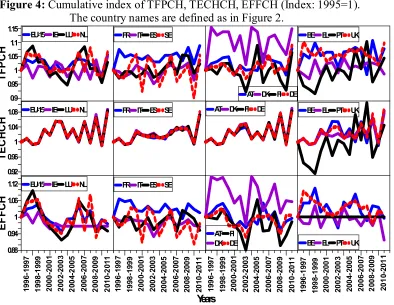
16 Figure 4: Cumulative index of TFPCH, TECHCH, EFFCH (Index: 1995=1).

The country names are defined as in Figure 2.

0.88 0.94 1 1.06 1.12 EF FC H 0.92 0.96 1 1.04 1.08 TE C HC H 0.9 0.95 1 1.05 1.1 1.15 TF PC H Years

EU-15 IE LU NL

19 96 -1 99 7 19 98 -1 99 9 20 00 -2 00 1 20 02 -2 00 3 20 04 -2 00 5 20 06 -2 00 7 20 08 -2 00 9 20 10 -2 01 1 19 96 -1 99 7 19 98 -1 99 9 20 00 -2 00 1 20 02 -2 00 3 20 04 -2 00 5 20 06 -2 00 7 20 08 -2 00 9 20 10 -2 01 1 19 96 -1 99 7 19 98 -1 99 9 20 00 -2 00 1 20 02 -2 00 3 20 04 -2 00 5 20 06 -2 00 7 20 08 -2 00 9 20 10 -2 01 1 19 96 -1 99 7 19 98 -1 99 9 20 00 -2 00 1 20 02 -2 00 3 20 04 -2 00 5 20 06 -2 00 7 20 08 -2 00 9 20 10 -2 01 1

FR IT ES SE

AT DK FI DE

BE EL PT UK

EU-15 IE LU NL FR IT ES SE AT DK FI DE BE EL PT UK

EU-15 IE LU NL FR IT ES SE

AT

DK FIDE BE EL PT UK

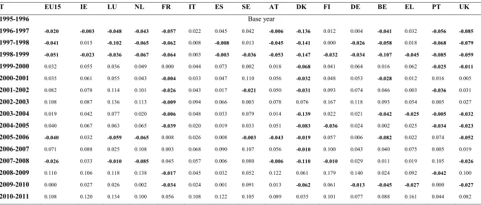
Detailed observations of Figure 4 are included in Table 1. Table 1 reports for each

country and each year, when productivity gains are a result of an improvement in

efficiency or not; and also, when there is a technological progress/loss and a productivity

progress/loss. Table 1 is constructed through a step-by-step procedure until the final

results are obtained. The procedure is as follows:

The first step is to determine the difference between the two indexes of TECHCH

and EFFCH. As it was mentioned before, productivity change is mainly derived from an

improvement in efficiency (EFF) (this occurs when TECHCH-EFFCH<0). Also,

productivity change is mainly the result of technological progress (TECH) (when

TECHCH-EFFCH>0). If there is no difference between TECHCH and EFFCH, the

17

During the period under consideration, the difference between the two indexes of

TECHCH and EFFCH for the entire EU15 and for each of the individual EU15 countries

can be negative, positive or zero (see Table A1 in the Appendix).

From the obtained results we observe that the frequency of occurrence of negative

value (TECHCH-EFFCH<0) is: twelve times in the case of Denmark, ten times in the

case of France, nine times in the case of the United Kingdom, eight times in the case of

Portugal, seven times in the case of Belgium, five times in the cases of the entire EU15,

Luxembourg, Netherlands and Austria, three times in the cases of Sweden, Finland,

Germany and Greece, two times in the cases of Ireland and Spain and zero times in the

case of Italy.

In this case (negative difference between the two indexes of TECHCH and

EFFCH) the productivity change is mainly derived from an improvement in efficiency

(EFF).

DMUs with an incidence of at least 7 times negative value

(TECHCH-EFFCH<0), show a negative average (France: -0.014, Denmark: -0.054, Belgium: -0.006,

Portugal: -0.007, United Kingdom:-0.009). Therefore, these countries have mainly

invested in methods to improve efficiency, through appropriate energy policies and

regulations.

The frequency of occurrence of positive value (TECHCH-EFFCH>0) is: fifteen

times in the case of Italy, thirteen times in the cases of Ireland and Spain, twelve times in

the cases of Sweden, Germany and Greece, eleven times in the case of Finland, ten times

18

nine times in the case of the entire EU15, six times in the cases of Portugal and the United

Kingdom, four times in the case of France and three times in the case of Denmark

In this case (positive difference between the two indexes of TECHCH and

EFFCH) the productivity change is mainly the result of technological progress (TECH).

DMUs with an incidence of at least 9 times positive value (TECHCH-EFFCH>0),

show a positive average(the entire EU-15: 0.0285, Ireland: 0.0523, Luxembourg: 0.0353,

Netherlands: 0.0276, Italy: 0.0429, Spain: 0.0365, Sweden: 0.0438, Austria: 0.0263,

Finland: 0.0535, Germany: 0.0387, Greece: 0.0319). Therefore, these countries have

mainly invested in methods to improve technology, through appropriate energy policies

and regulations.

The frequency of occurrence of zero value (TECHCH=EFFCH) is: one time in the

cases of the entire EU15, France, Finland and Portugal. In this case (no difference

between the two indexes of TECHCH and EFFCH) the productivity change is the result

of both technological progress (TECH) and efficiency improvement (EFF).

At this point it should be noted that, for all EU-15 countries except Italy, the

values (TECHCH-EFFCH) in different spans of time are alternating between positive and

negative ones. When the time span with a homogenous pattern (numbers with the same

sign) is long, then there is a short-term effort for energy policy stabilization in one

direction, geared towards an improvement in efficiency (EFF) or towards a technological

progress (TECH). In that respect, alternation exists when a policy is not performing as

expected. When the time span with a homogenous pattern (numbers with the same sign)

is short (one or two years), then there is a mild policy without clear orientation towards

19

The main objective of the energy strategy and policy is to provide a short-term

plan for rehabilitation of the energy sector. Furthermore, it gives the directions for the

medium to long-term reconstruction of the energy sector. The energy strategy shows how

DMUs can use their energy resources to achieve economic and social benefits in an

environmentally responsible manner. It gives the directions and the objectives of

comprehensive and inclusive policy geared towards an improvement in efficiency (EFF)

or towards a technological progress (TECH) or towards a combination of the two.

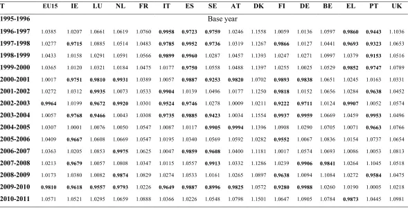
The second step of our analysis is to see if the Malmquist Productivity Index

between two periods t and t+1 is greater than 1, smaller than 1 or remains unchanged in

the case of the entire EU15 and for each individual EU15 country (see Table A2 in the

Appendix).

In terms of productivity change from one year to the next and under constant

returns to scale, an improvement of productivity can be the result of a single factor, or a

combination of two factors known as technical change (technological progress) and

efficiency change (improvement in efficiency). For example, one DMU may increase its

productivity solely by technical change and with no change of the distance to the

respective frontier. In other cases, the productivity change is a combination of technical

change and technical efficiency change. To summarize, productivity change can be a

result of technical change, technical efficiency change or a combination of the two.

During the period under consideration, the total factor productivity index (see

Table A2 in the Appendix) for the entire EU15 and for each of the individual EU15

countries can be greater or smaller than one. The frequency of occurrence of total factor

20

 in the case of entire EU15, TFPCH index is 13 (2) times greater (smaller) than one

 in the case of Ireland, TFPCH index is 9 (6) times greater (smaller) than one

 in the cases of Luxembourg, Netherlands, Germany and Greece, TFPCH index is 10

(5) times greater (smaller) than one

 in the cases of France, Denmark and the United Kingdom, TFPCH index is 15 times

greater than one (the whole sample period)

 in the case of Italy, index of TFPCH is 8 (7) times greater (smaller) than one

 in the case of Spain, the index of TFPCH is 6 (9) times greater (smaller) than one

 in the cases of Sweden , Finland and Portugal, the index of TFPCH is 7 (8) times

greater (smaller) than one

 in the case of Austria, the index of TFPCH is 12 (3) times greater (smaller) than one

 in the case of Belgium, the index of TFPCH is 14 (1) times greater (smaller) than one

It should be mentioned that in the case where the total factor productivity index

between time periods t and t+1 is greater than 1, the energy consumption performance

improves (productivity gains). On the other hand, when the total factor productivity index

between two time periods t and t-+1 is smaller than 1, then the energy consumption

performance declines (productivity loss).

Combining the above two steps, the final results of Table 1 are obtained. Τhis

table shows for each country and each year: i) the productivity gains (TFPCH>1) as a

result of improvements in efficiency (TECHCH-EFFCH<0) and technological progress

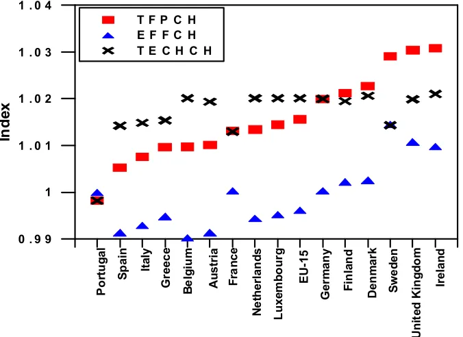
21 Table 1: Productivity gains as a result of improvements in efficiency and technological progress and productivity loss. Country names

are defined in Figure 2

t EU15 IE LU NL FR IT ES SE AT DK FI DE BE EL PT UK

1995-1996 Base year

1996-1997 EFF (a) _{EFF EFF EFF EFF TECH}L (b) _TECHL _TECHL _{EFF EFF TECH}(c) _{TECH EFF TECH}L _EFFL (d) _EFF

1997-1998 EFF TECHL EFF EFF EFF TECHL EFFL TECHL EFF EFF EFF L_=TECHL

(e) EFF EFF TECHL EFFL EFF

1998-1999 EFF EFF EFF EFF EFF TECHL _EFFL _{EFF EFF EFF EFF EFF EFF EFF EFF}L _EFF

1999-2000 TECH TECH TECH TECH EFF=TECH (f) _{TECH TECH}L _{TECH TECH EFF TECH TECH TECH TECH}L _EFFL _EFF

2000-2001 TECH TECHL TECHL TECHL EFF TECH TECHL TECHL TECHL EFF TECHL TECHL EFF TECH TECH TECH

2001-2002 TECH TECH TECHL TECH EFF TECHL TECH EFF TECH EFF TECHL TECH TECH TECH EFFL TECH

2002-2003 TECHL _TECH TECH

L TECHL EFF TECHL TECHL TECH TECH TECH TECHL TECHL TECH TECHL TECH TECH

2003-2004 TECH TECHL TECHL TECH EFF TECHL TECHL TECHL TECH EFF TECHL TECHL EFF EFF EFFL EFF

2004-2005 TECH TECH TECH TECH EFF TECH TECH TECHL _TECHL _{EFF EFF TECH TECH TECH EFF}L _EFF

2005-2006 EFF TECHL EFF EFF TECH TECH TECH EFF EFF EFF TECHL TECH EFF TECH TECH EFF

2006-2007 TECH TECH TECH TECHL _{TECH TECH TECH}L _TECHL _{TECH EFF TECH TECH TECH TECH TECH TECH}

2007-2008 EFF TECHL EFF EFF TECH TECH TECH TECHL EFF EFF EFF TECHL TECHL TECH TECH EFF

2008-2009 TECH TECH TECH TECHL _{EFF TECH TECH TECH TECH TECH TECH}L _{TECH TECH TECH EFF}L _TECH

2009-2010 EFFL=TECHL TECHL TECHL TECHL EFF TECHL TECHL TECHL TECHL EFF TECHL EFFL EFF EFF EFF=TEC_H EFF

2010-2011 TECH TECH TECH TECH TECH TECH TECH TECH TECH TECH TECH TECH TECH TECHL _{TECH TECH}

a_{EFF: Productivity gains as a result of improvements in Efficiency,} b_TECHL_{: Technological Progress but productivity losses,} c_{TECH: Productivity gains as a}

result of Technological Progress, d_EFFL_{: Improvements in Efficiency but productivity losses,} e_EFFL_=TECHL_{: Efficiency change is equal to technological}

22 5. Discussion

The next step of our analysis aims to provide an extra insight into assessing

relative productivity. Taking into account the empirical results obtained in the previous

section, we have a deeper understanding of the content of productivity changes among

cross-country comparisons. This provides policy makers with more valuable reference

material related to drawing up policies that aim to increase national productivity.

Therefore, based on Figure 2, the eco-inefficiency score indicates the evaluated

DMU’s distance from the best practice DMUs with different production mixes to the

efficient frontier. The best practice DMUs (Ireland 2000, Italy 2000, Austria 2000,

France 2000, Ireland 2009 and Sweden 2009) appear equally attractive for inefficient

DMU, which has the flexibility to choose an improvement direction that maximizes its

efficiency. The DMUs with a high eco-efficiency are those situated in the upper right

corner of the two frontiers of Figure 2, where they produce higher desirable outputs with

the lowest undesirable outputs. These countries are France 2000 and Sweden 2009. The

DMUs located on the frontier are considered eco-efficient, because no other DMUs can

produce more desirable outputs and fewer undesirable outputs.

If a DMU fails to achieve an output combination on its production possibility

frontier and falls beneath this frontier, then it is said to be technically inefficient, as it gets

further away from the more efficient countries (e.g. Belgium 2000/2009, Greece

2000/2009, Netherlands 2000/2009).

In Figure 2, technological progress shifts upwards the production possibility

frontier, as more outputs are obtainable using the same level of inputs. It can be seen

23

progress from 2000 to 2009, as in the case of Sweden. In the absence of technological

progress or improvement, an economy (e.g. Greece, Belgium, Netherlands) is found more

and more far from the best practice countries, or driven to the simultaneous increase

(Luxembourg, Finland) or decrease (Italy) of both GDP production and CO2 emissions

(Figure 3).

The simultaneous increase of GDP production (desirable output) and decrease of

CO2 emissions (undesirable output) can only be achieved through technical progress that

affect the ability to optimally combine inputs and outputs.

Combining the results depicted in Figure 2 and Figure 3, one can see whether the

use of input (total energy consumption) or CO2 emissions is the driving force of

productivity growth. Therefore, an overall conclusion can be drawn regarding whether

the overall development is driven by input-saving or by environmental-saving factors.

As shown in Figure 4 and Table 1, the detailed decomposition of total factor

productivity change offers additional insights for policy implications, representing the

driving forces of productivity gains or losses for the entire EU15 and for each of the

individual EU15 countries. Therefore, it illustrates the nature of the overall productivity

change that shapes up the Malmquist index.

More specifically, from this analysis one can see when the possible effect is

characterized as EFF (productivity gains as a result of improvement in efficiency), TECH

(productivity gains as a result of technological progress), EFFL _{(improvement in}

efficiency but productivity losses), TECHL (technological progress but productivity

24

productivity gains), and EFFL=TECHL (efficiency change is equal to technological

change in the case of productivity losses) (see Table 1).

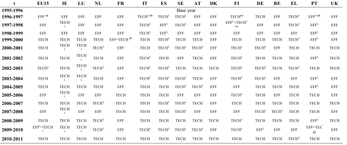
Figure 5 reports the average values of the Malmquist (TFPCH) index and its

components (EFFCH, TECHCH) for the EU15 countries. The greatest increases of the

TFPCH index are observed in Ireland, UK and Sweden, whereas the lowest ones in

Portugal, Spain and Italy.

Figure 5: Annual means of Malmquist index and its components. Countries are sorted in

ascending order by the TFPCH index.

0 . 9 9 1 1 . 0 1 1 . 0 2 1 . 0 3 1 . 0 4

In

de

x

T F P C H E F F C H T E C H C H

Ire la nd Po rtu ga l Sp ai n Ita ly G re ec e Be lg iu m A us tr ia Fr an ce Ne th er la nd s Lu xe m bo ur g EU -1 5 G er m an y Fi nl an d D en m ar k U ni te d K in gd om Sw ed en

The analysis of efficiency changes (EFFCH) shows that, the average

eco-efficiency change is positive (higher than one) for 7 of 16 DMUs. These are Sweden, UK,

Ireland, Denmark, Finland, Germany and France, indicating that these DMUs have

caught up the eco-efficiency benchmarks.

From the above countries, Sweden, UK, Ireland and Denmark, have the highest

25

energy, through gradual substitution procedures between fossil and non fossil fuels. The

more a DMU abstains from the consumption of fossil fuels, the greater the divergence

between the desirable (GDP) and the undesirable output (CO2) (see also Figure 1). This

happens because the maximization of the desirable output (GDP) comes with the

temporal stabilization or decrease of the undesirable byproduct. This procedure is related

to how effective is the energy mix and, therefore, how effectively the inputs are

transformed into outputs using the available technology.

However, it is the average technical change that contributes most to productivity

gains (TFPCH) (Figure 5), as it describes the change of the frontier (Figure 3) and,

therefore, the best performers of the sample and not the development of the DMUs under

the frontier (Figure 2). Our results are similar to those reported in the study conducted by

Makridou et al. (2016), who concluded that technology change is primarily responsible

for the improvements achieved in most sectors.

The results of the model show that the average TECHCH index is positive

(higher than one) and greater than the average EFFCH index in all countries, except

Portugal where there is an average decrease of 0.18% in the sample period.

The results on Figure 5 suggest that if the annual average growth of EFFCH is

higher than one and lower than the annual average growth of TECHCH, then productivity

gain (TFPCH), which is primarily the result of technological progress, have the highest

value. Thus, the best DMUs of the sample, with the highest values of TFPCH index, are

identified in the case of Ireland, United Kingdom, Sweden, Denmark, Finland and

Germany. In the case of Sweden, the annual average growth of EFFCH (1.45%) is almost

26

On the other hand, if the annual average growth of EFFCH is lower than one and

lower than the annual average growth of TECHCH, which is higher than one, then

productivity gain (TFPCH), which is primarily the result of technological progress, have

the lowest value. Thus, the worst DMUs of the sample with the lowest values of TFPCH

index are identified in the case of EU15, Luxembourg, Netherlands, France, Austria,

Belgium, Greece, Italy and Spain. In the case of France, the annual average growth of

EFFCH is positive (higher than one) with an average increase of 0.03% (Figure 5).

6. Conclusions and policy implications

This study develops an input oriented DEA model, aggregating both energy

productivity and environmental degradation into a comprehensive index of Total Factor

Productivity (Malmquist), in order to evaluate a DMU’s total factor productivity.

The results suggest that technical progress affecting the ability to optimally

combine inputs and outputs is the main factor for the simultaneous increase of desirable

output and decrease of undesirable byproduct for most DMUs for the sample period

under examination. In the absence of technical progress, a DMU is either far from the

best practice DMUs (e.g. Greece, Belgium, Netherlands), or driven to the simultaneous

increase (Luxembourg, Finland) or decrease (Italy) of both GDP production and CO2

emissions.

An assessment of each DMU’s productivity for the sample period is summarized

in the following cases:

i) Productivity gains are due to an improvement in efficiency,

27

iii) There is an improvement in efficiency, but the productivity decreases,

iv) There is technological progress, but the productivity decreases,

v) There are productivity gains when efficiency change is equal to technological change,

vi) There is productivity loss when efficiency change is equal to technological change.

As shown from the analysis, the highest values of productivity gains (TFPCH) can

be achieved in the case where the annual average growth of EFFCH is higher than one

and lower than the annual average growth of TECHCH (Ireland, United Kingdom,

Sweden, Denmark, Finland, Germany). On the other hand, the lowest values of

productivity gains (TFPCH) appears when the annual average growth of EFFCH is lower

than one and lower than the annual average growth of TECHCH (EU15, Luxembourg,

Netherlands, France, Austria, Belgium, Greece, Italy and Spain).

The methodology utilized here and the results obtained capture the different

causes of losses or gains in DMU’s productivity from year to year. This work quantifies

the inefficiency of the DMUs under the frontier, through the indicators of EFFCH,

TECHCH and TFPCH. Such an approach is of particular importance in encouraging

inefficient DMUs to always compare themselves with efficient DMUs in their range, and

thus to make progress and improvements.

The obtained results have important implications for the policy makers to promote

productivity performance of the energy sector in EU-15 countries. The detailed

decomposition of productivity change into efficiency change, technology change,

innovation efficiency and technology catch-up effect offers a better understanding of the

content of the productivity change through the cross-country comparisons. That

28

EU15 and for each of the individual EU15 countries and thus offers additional insights

for policy implications. For instance, policy actions intended to improve productivity

gains (decrease productivity losses) might be misdirected if they focus (if they choose not

to focus) on accelerating the rate of innovation, in the case where the productivity gains

(productivity losses) are mainly the result of improvements in efficiency. Therefore, the

present study provides more reference material to policy makers so as to draw up policies

in order to elevate national productivity for the purpose of designing energy development

strategy in EU-15 countries.

In order to quantify the huge efficiency gap so as to address the wasteful use of

exhaustible energy inputs and reduce the environmental degradation, we calculate the

distance for an inefficient DMU to the production frontier, through the DEA based

Malmquist productivity index. In many cases, the distance of a specific DMU from the

best practice DMUs indicates different production combination of desirable and

undesirable outputs, and, therefore different alternatives for an inefficient DMU to choose

a direction that maximizes its efficiency. The direction that an inefficient DMU should

take and the amount of reduction of the energy consumption can be the basis for a

government to establish energy saving policies and to strengthen energy management,

especially in the cases where large amounts of energy input are necessary in the

economy, but with low value added. An energy management system is one of the most

important factors in the context of strengthening energy efficiency policy as it allows in

energy efficiency issues to gain a greater priority within the DMU.

This analysis allows policy makers of EU states to identify the explanatory causes

29

In this sense, it is very important to identify the economic activities that, due to their

impact, are essential to reduce energy consumption, as well as potential strategies and

measures to improve the efficiency of final energy use. For example, restructuring of

industry, developing programs of technology innovation and encouraging the reuse of

input resources can be some of the directions to follow in the context of strengthening

energy efficiency policies.

It is necessary for policy makers to promote technological innovation on energy

saving and emission reduction. To realize this purpose, it is absolutely essential to

increase research investment to develop environmental technology, energy saving

technology and low-carbon technology in order to limit excessive energy consumption

and pollutant emissions.

In this way, technological innovation has an additive significant contribution on

strategies of optimizing industrial structure as it manages to accelerate the development

of environmental-friendly industries.

Thus, the results obtained here can be used as a guide for policy makers to

promote the best efficiency measures for a given level of resources use over the same

period. Furthermore they can serve as a useful tool for policy making by investigating the

gradual process of the diffusion and adoption of new technologies. Also, they can be used

to optimize the management of energy resources in order to achieve the highest

30 References

Apergis, Nicholas, Goodness C. Aye, Carlos Pestana Barros, Rangan Gupta, and Peter Wanke. (2015). Energy efficiency of selected OECD countries: A slacks based model

with undesirable outputs, Energy Economics 51: 45-53.

Bampatsou, Christina, and George Hadjiconstantinou. (2009). The use of the DEA method for simultaneous analysis of the interrelationships among economic growth,

environmental pollution and energy consumption, International Journal o f Economic

Sciences and Applied Research 2 (2): 65-86.

Bampatsou, Christina, Savas Papadopoulos, and Efthimios Zervas. (2013). Technical efficiency of economic systems of EU-15 countries based on energy consumption. Energy Policy 55: 426-434.

Bevilacqua, Maurizio, and Marcello Braglia. (2002). Environmental efficiency analysis

for ENI oil refineries, Journal of Cleaner Production 10 (1): 85–92.

Caves, Douglas W., Laurits R. Christensen, and W. Erwin Diewert. (1982). The Economic Theory of Index Numbers and the Measurement of Input, Output, and

Productivity. Econometrica 50(6): 1393–1414.

Chames, Abraham, William W. Cooper, and Edwardo L. Rhodes. (1978). Measuring the

efficiency of decision making units. European Journal of Operational Research 2

(6):429-444.

Charnes, Abraham, William W. Cooper, Arie Y. Lewin, and Lawrence M. Seiford.

(1993). Data Envelopment Analysis: Theory, methodology, and application, Boston:

Kluwer Academic Publishers.

Chen, Chien-Ming, and Magali A. Delmas. (2012).“Measuring Eco-inefficiency: A New

Frontier Approach, Operations Research 60: 1064–1079.

Corrado, Carol, Hulten Charles, and Daniel Sichel. (2005). “Measuring Capital and

Technology: An Expanded Framework,” in Measuring Capital in the New Economy,

C. Corrado, J. Haltiwanger, and D. Sichel, (Eds.), Studies in Income and Wealth, 65: 11-41, Chicago: The University of Chicago Press for the National Bureau of Economic Research.

http://econweb.umd.edu/~hulten/webpagefiles/Measuring%20Capital%20and%20Tec hnology%20%20An%20Expanded%20Framework.pdf

Corrado, Carol, Charles Hulten, and Daniel Sichel. (2009). “Intangible Capital and U.S.

31

EIA. (2013). International Energy Annual. Energy Information Administration, U.S.

Department of Energy. http://www.eia.doe.gov/iea/contents.html [accessed date: 06

October, 2013].

Fagerberg, Jan. (1994). Technology and International Differences in Growth

Rates, Journal of Economic Literature 32(3): 1147–1175.

Färe, Rolf, and C. A. Knox Lovell. (1978). Measuring the technical efficiency of

production, Journal of Economic Theory 19 (1): 150-162.

.

Färe, Rolf., Shawna Grosskopf, and C. A. Knox Lovell. (1994a). Production Frontiers,

Cambridge: Cambridge University Press.

Färe, Rolf, Shawna Grosskopf, Mary Norris, and Zhongyang Zhang. (1994b). Productivity Growth, Technical Progress, and Efficiency Change in Industrialized

Countries, The American Economic Review 84(1): 66–83.

Färe, Rolf, Shawna Grosskopf, and Pontus Roos. (1995). Productivity and quality

changes in Swedish pharmacies, International Journal of Production Economics 39

(1–2): 137-144.

Farrell, Michael J. (1957). The Measurement of Productive Efficiency, Journal of the

Royal Statistical Society. Series A (general)120(3): 253-290.

Fischer, Manfred M., Thomas Scherngell, and Martin Reismann. (2009). Knowledge spillovers and total factor productivity: evidence using a spatial panel data model, Geographical Analysis 41(2): 204–220.

Fixler, Dennis, and Kimberly D. Zieschang. (1992). “Incorporating Ancillary Measures

of Process and Quality Change into a Superlative Productivity Index,” Journal of

Productivity Analysis 2(4): 245-267.

Fried, Harold O., C. A. Knox Lovell, and Shelton S. Schmidt, (2008). The Measurement

of Productive Efficiency and Productivity Change, New York: Oxford University

Press.

Fukuyama, Hirofumi, Hiroya Masaki, Kazuyuki Sekitani, and Jianming Shi. (2013). Distance optimization approach to ratio-form efficiency measures in data envelopment

analysis, Journal of Productivity Analysis 42(2): 175-186.

Golany, Boaz, and Sten Thore. (1997). The economic and social performance of nations:

32

Halkos G. (2010). Construction of abatement cost curves: The case of F-gases, MPRA

Paper 26532, University Library of Munich, Germany.

Halkos G. (2014). The Economics of Climate Change Policy: Critical review and future

policy directions, MPRA Paper 56841, University Library of Munich, Germany.

Halkos G and Salamouris (2004). Efficiency measurement of the Greek commercial banks with the use of financial ratios: a data envelopment analysis approach.

Management Accounting Research 15 (2): 201-224.

Halkos G. and Tsilika K. (2014). Analyzing and visualizing the synergistic impact

mechanisms of climate change related costs, MPRA Paper 55459, University Library

of Munich, Germany.

Halkos G. and Tsilika K. (2016). Climate change impacts: Understanding the synergetic

interactions using graph computing, MPRA Paper 75037, University Library of

Munich, Germany.

Halkos G. and Paizanos E. (2016). The effects of fiscal policy on CO2 emissions: Evidence from the U.S.A, Energy Policy, 88(C), 317-328.

Halkos G. and Polemis M. (2016). The good, the bad and the ugly? Balancing

environmental and economic impacts towards efficiency, MPRA Paper 72132,

University Library of Munich, Germany.

Halkos G. and Skouloudis A. (2015). Exploring corporate disclosure on climate change:

Evidence from the Greek business sector, MPRA Paper 64566, University Library of

Munich, Germany.

Kitcher, Ben, Ian P. McCarthy, Sam Turner, and Keith Ridgway. (2013). Understanding

the effects of outsourcing: unpacking the total factor productivity variable, Production

Planning & Control:The management of Operations 24 (4-5): 308–317.

Kortelainen, Mika. (2008). Dynamic environmental performance analysis: A Malmquist

index approach, Ecological Economics 64(4): 701–715.

.

Kuo, Renjieh J., Y. C. Wang, and Fanchih C. Tien. (2010). Integration of artificial neural

network and MADA methods for green supplier selection, Journal of Cleaner

Production 18(12): 1161–1170.

Long, Xingle, Xicang Zhao, and Faxin Cheng. (2015). The comparison analysis of total

factor productivity and eco-efficiency in China's cement manufactures, Energy Policy

81: 61-66.

Mahlberg, Bernhard, Mikulas Luptacik, and Biresh K. Sahoo. (2011). Examining the drivers of total factor productivity change with an illustrative example of 14 EU

33

Makridou, Georgia, Kostas Andriosopoulos, Michael Doumpos, and Constantin Zopounidis. (2015). A Two-stage approach for energy efficiency analysis in European

Union countries, The Energy Journal 36 (2): 47-69.

Makridou, Georgia, Kostas Andriosopoulos, Michael Doumpos, and Constantin Zopounidis. (2016). Measuring the efficiency of energy-intensive industries across

European countries, Energy Policy 88: 573-583.

Malmquist, Sten. (1953). Index numbers and indifference surfaces, Trabajos de

Estadistica 4(2) : 209-242.

Murillo-Zamorano, Luis R. (2005). The Role of Energy in Productivity Growth: A

Controversial Issue?, The Energy Journal 26 (2): 69-88.

10.5547/ISSN0195-6574-EJ-Vol26-No2-4

OECD. (2013). Gross Domestic Product (GDP) in national currency, in current prices and constant prices (national base year, previous year prices and OECD base year i.e.

2005), Organisation for Economic Co-operation and Development.

http://stats.oecd.org/ [accessed date: 04 October, 2013].

Pardo Martínez, Clara I. (2013). An analysis of eco-efficiency in energy use and CO2

emissions in the Swedish service industries, Socio-Economic Planning Sciences

47(2):120-130.

Ramanathan, Ramakrishnan. (2006). A multi-factor efficiency perspective to the relationships among world GDP, energy consumption and carbon dioxide emissions,

Technological Forecasting and Social Change 73(5): 483-494.

http://dx.doi.org/10.1016/j.techfore.2005.06.012.

Ramli, Noor Asiah., and Susila Munisamy. (2013). A Study on Eco-Efficiency of the

Manufacturing Sector in Malaysia, Actual Problems of Economics 12(150): 480- 491.

http://repository.um.edu.my/30015/1/A%20Study%20on%20Eco- Efficiency%20of%20the%20Manufacturing%20Sector%20in%20Malaysia%20-%20postprint.pdf.

Sarkis, Joseph, and Jeffrey Weinrach. (2001). Using data envelopment analysis to

evaluate environmentally conscious waste treatment technology, Journal of Cleaner

Production 9(5): 417-427.

Sheng, Yu, Yanrui Wu, Xunpeng Shi, and Dandan Zhang. (2015). Energy trade

efficiency and its determinants: A Malmquist index approach, Energy Economics 50:

306-314.

Shephard, Ronald W. (1970). Theory of Cost and Production Functions. Princeton, New

34

Shephard, Ronald W., and Rolf Färe. (1974). “The law of diminishing returns,” Zeitschrift für Nationalökonomie 34 (1): 69–90.

Sueyoshi, Toshiyuki, and Yan Yuan. (2016). Marginal Rate of Transformation and Rate of Substitution Measured by DEA Environmental Assessment: Comparison among

European and North American Nations, Energy Economics. 56(C): 270-287.

Wang, Ke, and Yi-Ming Wei. (2016). Sources of energy productivity change in China during 1997–2012: A decomposition analysis based on the Luenberger productivity

indicator, Energy Economics 54:50-59.

Xishuang, Han, Xue Xiaolong, Ge Jiaoju, Wu Hengqin, and Su Chang. (2014). Measuring the Productivity of Energy Consumption of Major Industries in China: A

DEA-Based Method, Mathematical Problems in Engineering 2014. http://dx.doi.