Simulating low frequency changes in atmospheric CO

www.clim-past.net/2/57/2006/

© Author(s) 2006. This work is licensed under a Creative Commons License.

Climate

of the Past

Simulating low frequency changes in atmospheric CO

2

during the

last 740 000 years

P. K¨ohler and H. Fischer

Alfred Wegener Institute, Helmholtz Center for Polar and Marine Research, P.O. Box 12 01 61, 27515 Bremerhaven, Germany Received: 15 December 2005 – Published in Clim. Past Discuss.: 14 February 2006

Revised: 3 July 2006 – Accepted: 1 September 2006 – Published: 11 September 2006

Abstract. Atmospheric CO2measured in Antarctic ice cores shows a natural variability of 80 to 100 ppmv during the last four glacial cycles and variations of approximately 60 ppmv in the two cycles between 410 and 650 kyr BP. We here use various paleo-climatic records from the EPICA Dome C Antarctic ice core and from oceanic sediment cores cover-ing the last 740 kyr to force the ocean/atmosphere/biosphere box model of the global carbon cycle BICYCLEin a forward mode over this time in order to interpret the natural variabil-ity of CO2. Our approach is based on the previous interpreta-tion of carbon cycle variainterpreta-tions during Terminainterpreta-tion I (K¨ohler et al., 2005a). In the absense of a process-based sediment module one main simplification of BICYCLEis that carbon-ate compensation is approximcarbon-ated by the temporally delayed restoration of deep ocean [CO2₃−]. Our results match the low frequency changes in CO2 measured in the Vostok and the EPICA Dome C ice core for the last 650 kyr BP (r2≈0.75). During these transient simulations the carbon cycle reaches never a steady state due to the ongoing variability of the over-all carbon budget caused by the time delayed response of the carbonate compensation to other processes. The aver-age contributions of different processes to the rise in CO2 during Terminations I to V and during earlier terminations are: the rise in Southern Ocean vertical mixing: 36/22 ppmv, the rise in ocean temperature: 26/11 ppmv, iron limitation of the marine biota in the Southern Ocean: 20/14 ppmv, car-bonate compensation: 15/7 ppmv, the rise in North Atlantic deep water formation: 13/0 ppmv, the rise in gas exchange due to a decreasing sea ice cover: −8/−7 ppmv, sea level rise: −12/−4 ppmv, and rising terrestrial carbon storage: −13/−6 ppmv. According to our model the smaller inter-glacial CO2values in the pre-Vostok period prior to Termi-nation V are mainly caused by smaller interglacial Southern Ocean SST and an Atlantic THC which stayed before MIS 11 (before 420 kyr BP) in its weaker glacial circulation mode.

Correspondence to: P. K¨ohler ([email protected])

1 Introduction

Paleo-climatic records derived from ice cores revealed the natural variability in Antarctic temperature (Jouzel et al., 1987), atmospheric dust content (R¨othlisberger et al., 2002), and atmospheric CO2 (Barnola et al., 1987; Fischer et al., 1999; Petit et al., 1999; Monnin et al., 2001; Kawamura et al., 2003; Siegenthaler et al., 2005) over the last glacial cycles. The longest CO2record from the Antarctic ice core at Vos-tok (Petit et al., 1999) went back in time as far as about 410 kyr BP showing a switch of glacials and interglacials in all those parameters approximately every 100 kyr during the last four glacial cycles with CO2varying between 180– 300 ppmv. New measurements of dust and the isotopic tem-perature proxy δD of the EPICA Dome C ice core cover-ing the last 740 kyr, however, revealed previous glacial cy-cles of reduced temperature amplitude (EPICA-community-members, 2004). These new archives offered the possibility to propose atmospheric CO2 for the pre-Vostok time span as called for in the “EPICA challenge” (Wolff et al., 2004). Here, we contribute to this challenge using BICYCLE, a box model of the isotopic carbon cycle which is based on the interpretation of glacial/interglacial variability of the carbon cycle during Termination I (K¨ohler et al., 2005a).

ocean are processes affecting the carbon cycle via the physi-cal pump. The fertilisation of the marine biologiphysi-cal produc-tivity through the aeolian input of iron in areas of high nitrate and low chlorophyll (HNLC) is one theory (Martin, 1990; Ridgwell, 2003b) which would reduce atmospheric CO2 dur-ing glacial times through an enhanced biological export pro-duction to the deep ocean. The export of organic carbon it-self is closely coupled to the calcium carbonate production of pelagic calcifiers by which CO2 is released in the sur-face ocean. Additionally to those processes which distribute DIC, alkalinity and nutrients in the different ocean reser-voirs, fluxes of carbon between the terrestrial biosphere and the ocean/atmosphere system (e.g. Joos et al., 2004), river-ine input of bicarbonate (Munhoven, 2002), and exchange fluxes of DIC and alkalinity via dissolution and sedimenta-tion of CaCO3between ocean and sediments (e.g. Zeebe and Westbroek, 2003) need to be considered to fully understand glacial/interglacial changes in the global carbon cycle.

Previously we put forward a quantitative interpretation of observed changes in atmospheric CO2 and its carbon iso-topes (δ13C,114C) using the multi-box model of the global carbon cycle, called BICYCLE, applied to the last glacial ter-mination (K¨ohler et al., 2005a). That study concluded that the main processes impacting on CO2 during Termination I were an increase in vertical mixing rates in the South-ern Ocean and changes in the DIC and alkalinity inventories through sedimentation and dissolution processes. The time-dependent atmosphericδ13C record from the Taylor Dome ice core (Smith et al., 1999) used in that study contains valu-able informations, which envalu-abled us to reduce the uncertain-ties in determining the magnitude and timing of various pro-cesses. These results are in that sense robust that the detailed magnitudes of individual processes might vary due to model limitation and data uncertainties, but all their contributions need to be taken into account for explaining the observed variations in the atmospheric carbon records. The novelty of our approach is the simulation in a transient mode. Most other approaches were comparing steady state simulations for different boundary conditions. Assuming that these pro-cesses are of general nature, we simulated CO2 variations with (nearly) the same model over the time period of the last 740 kyr covered by the EPICA Dome C records which repre-sents our contribution to the “EPICA challenge” (Wolff et al., 2005). To this end we forced our model by proxy data from marine and ice core archives. We follow with a sensitivity analysis of the model and discuss its uncertainties.

2 Methods

2.1 The BICYCLEmodel

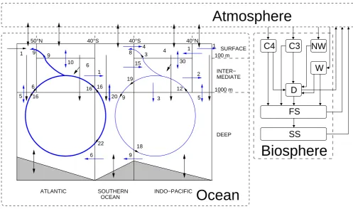
The Box model of the Isotopic Carbon cYCLE BICYCLE (K¨ohler et al., 2005a) was developed and applied for quan-titative interpretation of the atmospheric carbon records

(CO2, δ13C,114C) during Termination I (10−20 kyr BP). The model consists of ten oceanic reservoirs in three dif-ferent depth layers and distinguishes Atlantic, Indo-Pacific and Southern Ocean (Fig. 1). The strength of the preindus-trial ocean circulation as seen in Fig. 1 was parameterised with data from WOCE (Ganachaud and Wunsch, 2000). Ma-rine global export production of 10 PgC yr−1 at 100 m wa-ter depth (e.g. Gnanadesikan et al., 2002) was prescribed for the preindustrial setting, depending on the preformed macro-nutrient concentration of PO4in the surface waters. In the equatorial regions all macro-nutrients were utilised for the export production, while in the high latitudes the export pro-duction flux was restricted to avoid a global export flux of carbon which exceeds the prescribed 10 PgC yr−1. This led to unutilised nutrient concentrations especially in the South-ern Ocean, which can be used for increased marine produc-tivity during times of high aeolian iron input into these re-gions. The global preindustrial export of CaCO3 was set to 1 PgC (e.g. Jin et al., 2006) with a constant rain ratio of exported organic matter to CaCO3 of 10:1 throughout all our simulations. The remineralisation of organic matter in the abyss is assumed to follow the denitrification pathway if the deep ocean O2concentration drops below 4µmol kg−1, which is in line with the Ocean Carbon-Cycle Model Inter-comparison Project (OCMIP) 2 protocol. This implies that during further remineralisation no molecular oxygen is con-sumed and the model thus avoids unphysical conditions of negative O2concentration. During the carbonate compensa-tion (Broecker and Peng, 1987) the response of the sediments to changes in the deep ocean CO2₃−concentration ([CO2₃−]) is prescribed with a variable temporal delay (e-folding time

τ withτ between 0 and 6 kyr). In doing so we mimic the dissolution or sedimentation of CaCO3in the absence of a process-based module of early diagenesis (e.g. Archer et al., 1997, 1998). This leads to net changes in the inventories of DIC and alkalinity and therefore implicitly includes changes in the weathering inputs of bicarbonate through rivers. We are aware of the simplification of this approach, i.e. carbonate compensation in general is a response to balance anomalies in deep ocean [CO2₃−] caused by carbon cycle variability of the ocean/atmosphere/biosphere subsystem, the riverine in-put of alkalinity and its removal by sedimentation. However, while there are evidences for temporal changes in the riverine input rates of bicarbonate (Munhoven, 2002) we are aware of no proxy which can prescribe these changes and have there-fore chosen to represent riverine inputs only implicitly in our model. A globally averaged seven-compartment terrestrial biosphere (K¨ohler and Fischer, 2004) allows photosynthetic production of C3and C4pathways differing in their isotopic fractionation, and a climate and CO2-dependent fixation of carbon on land. A more detailed description of the model is found in K¨ohler et al. (2005a).

C3

FS

SS

W

D

C4

Atmosphere

Biosphere

NW

12

3 1

2 1 4

40°S 40°N

40°S 50°N

INTER− MEDIATE 1

DEEP 100 m

SURFACE

1000 m

ATLANTIC INDO−PACIFIC

6 9

9

19

9

18 15 8

6 9

1

16

22 16 16 6

4 3

30 10

20

SOUTHERN

OCEAN

Ocean

5 ₅

Fig. 1. Geometry of the Box model of the Isotopic Carbon cYCLE (BICYCLE). Carbon fluxes between different reservoirs are shown in black. Biosphere compartments: C4: C4ground vegetation; C3: C3ground vegetation; NW: non-woody parts of trees; W: woody parts of

trees; D: detritus; FS: fast decomposing soil; SS: slow decomposing soil. Ocean: Recent fluxes of ocean circulation (in Sv=106m3s−1) are shown in blue based on the World Ocean Circulation Experiment WOCE (Ganachaud and Wunsch, 2000). Bold arrows indicate those fluxes in ocean circulation which are changed over time (NADW formation and subsequent fluxes; Southern Ocean vertical mixing).

calculate the atmospheric partial pressure (pCO2inµatm). Only in dry air and at standard pressure, they are identical (Zeebe and Wolf-Gladrow, 2001). For reasons of simplic-ity we use throughout this article for both carbon dioxide data and simulation results the ice core nomenclature (CO2 in ppmv) and assume equality between both. This simplifica-tion neglects a relatively constant offset between both quan-tities of a few ppmv.

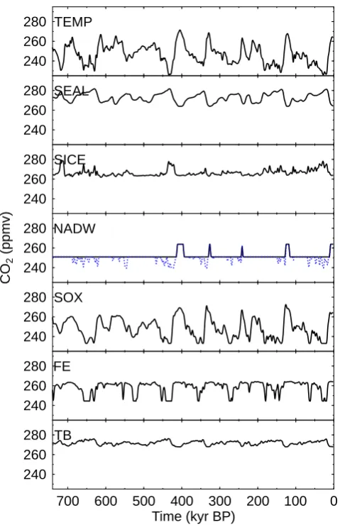
2.2 Time-dependent forcing of BICYCLE

We forced BICYCLE forward in time using various paleo-climatic records (Fig. 2). The model applied here used the same parameterisation as for its application on Termination I (K¨ohler et al., 2005a) with some exceptions: (1) We did not consider a complete shut-down of the North Atlantic Deep Water (NADW) formation during Heinrich events. This change is based on productivity results (Sachs and Ander-son, 2005) and sea level fluctuations (Siddall et al., 2003) that indicate that Heinrich events during MIS 2 and 3 may have caused different perturbations to the ocean circulation. It is therefore not possible to generalise changes in NADW formation throughout the EPICA Dome C period.

Neverthe-less, we discuss the potential impact of Heinrich events in Sect. 3.3. (2) While we previously prescribed the variability in the depth of the calcite saturation horizon we now assume a time delayed response of the carbonate compensation to changes in the deep ocean [CO2₃−]. (3) The aeolian input of iron into the Southern Ocean is now prescribed with an iron flux record published recently (Wolff et al., 2006), and not by the atmospheric dust concentration. The time-dependent forcing used here differs also in some aspects from our initial contribution to the EPICA challenge (Wolff et al., 2005).

Because various records that were used to force our model had a rather coarse resolution we have chosen to smooth all forcing records and all simulation results and concentrate on low frequency changes in the carbon cycle.

The relevant model forcings were used as described in the following:

0 20 40 60 80 100

IRD

(%)

(a)

5 10 15

SST

(

o C)

(b)

5 4 3 2

18

O

(

o /oo

)

(c)

0 -1 -2

18

O

(

o /oo

)

(d)

-15 -10 -5 0

T

(K)

(e)

1.0 0.5 0.0

1

8 O

(

o /o

o

)

(f)

-100 -50 0

sea

level

(m)

(g)

-450 -420 -390 -360

D

(

o /o

o

)

(h)

1 5

7 9

11 13 15

17

500 400 300 200 100 0

Fe

flux

(

g

m

-2

yr

-1 )

(i)

700 600 500 400 300 200 100 0

Time (kyr BP)

180 200 220 240 260 280

CO

2

(ppmv)

700 600 500 400 300 200 100 0

Time (kyr BP)

180 200 220 240 260 280 300

CO

2

(ppmv)

(j)

S6.0k S1.5k S0.0k

I II

III IV

V VI

VII VIII

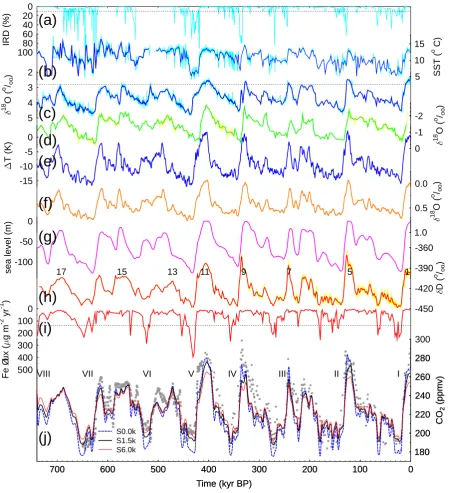
Fig. 2. Paleo-climatic records which were used to force the BICYCLEmodel (a–i) and measured and simulated CO2(j). Ice rafted debris IRD

(a), SST reconstructions (b), and benthicδ18O in foraminifers (c) from the sediment core drilled at the site ODP980 (55◦290N, 14◦420W) (McManus et al., 1999; Flower et al., 2000; Wright and Flower, 2002). (d): Plankticδ18O of ODP677 (1◦120N, 83◦440W) (Shackleton et al., 1990). Reconstructed (e) temperature changes over land in the northern hemisphere (40−80◦N), (f) variability in deep oceanδ18O caused by deep ocean temperature changes, and (g) sea level changes, (e–g) after Bintanja et al. (2005). Sea level corrected deuteriumδD (h) and atmospheric iron fluxes to Antarctica (i) as measured in the EPICA Dome C ice core (EPICA-community-members, 2004; Wolff et al., 2006). (j): Measured CO2from Vostok (grey circles) (Petit et al., 1999) plotted on the orbitally tuned age scale (Shackleton, 2000),

from EPICA Dome C (grey squares) (Siegenthaler et al., 2005), and simulated CO2(lines, 3 kyr running mean) of scenarios with different

to a glacial/interglacial amplitude during Termination I of 4 K (Fig. 2b). SSTs of equatorial surface oceans were estimated from planktic δ18O measured in ODP677 in the equatorial Pacific (Shackleton et al., 1990) scaled to a glacial/interglacial amplitude during Termination I of 3.75 K (Visser et al., 2003) (Fig. 2d). Southern Ocean (south of 40◦S) SST with a glacial/interglacial amplitude during Termination I of 4 K was estimated fromδD of the EPICA Dome C ice core (EPICA-community-members, 2004) (Fig. 2h). The EPICA Dome C δD was corrected for the effect of sea level changes (Jouzel et al., 2003) using a normalised record of sea level change from Bin-tanja et al. (2005). Deep ocean temperature changes are based on the temperature residual of the benthic δ18O (Fig. 2f) calculated by Bintanja et al. (2005) and scaled to a glacial/interglacial amplitude of 3 K (Labeyrie et al., 1987). Sea ice: Varying sea ice coverage will influence the gas exchange rates between the atmosphere and the surface ocean. We coupled time-dependent changes in the sea ice area in the North Atlantic and the Southern Ocean on the assumed temperature changes in the respective surface ocean boxes. Present day annual mean sea ice area was set to 10×1012m2 in each hemisphere (Cavalieri et al., 1997). During the LGM the annual average area covered by sea ice increased to 14×1012m2 in the North and 22×1012m2 in the South based on various studies (Crosta et al., 1998a,b; Sarnthein et al., 2003; Gersonde et al., 2005). In addition to changing surface box area due to sea level change this results in a relative areal coverage of 50 and 85% in the North Atlantic box and 13 and 30% in the Southern Ocean box during preindustrial times and the LGM, respectively. Sea level: We used the results of Bintanja et al. (2005) on changes in sea level (Fig. 2g). This modelling study is based on a benthicδ18O stack from 57 globally distributed sediment cores covering more than the last 5 million years (Lisiecki and Raymo, 2005). The sea level process com-bines what is normally called the “salinity effect” (glacial salinity which is about 3% higher than at preindustrial times) with a change in the concentration of DIC, alka-linity, nutrients, and oxygen in the ocean due to variable reservoir sizes. For each change in sea level the geom-etry (volume, surface area) of the oceanic reservoirs is revised based upon realistic bathymetric profiles calcu-lated from the Scripps Institute of Oceanography data set (http://dss.ucar.edu/datasets/ds750.1), which has a resolution of 1◦_×1◦_{and 1 m in the vertical direction.}

Ocean circulation: There are data- and model-based evidences for a reduced ocean overturning in the Atlantic and the Southern Ocean, while the glacial circulation in large parts of the Pacific Ocean seemed to have been similar to today (Meissner et al., 2003; Hodell et al., 2003; Knorr and Lohmann, 2003; Broecker et al., 2004; McManus

et al., 2004; Watson and Naveira-Garabato, 2006). It was shown (Flower et al., 2000) that the depth gradient inδ13C which is an indicator for the strength in NADW formation is highly correlated with benthic δ18O. To rely on as few different cores as possible and thus to minimise timing uncertainties we therefore used benthic δ18O in ODP980 (McManus et al., 1999; Flower et al., 2000) as a proxy for the strength in NADW formation bearing in mind that this might introduce a possible phase shift of the contribution of changes in NADW formation on CO2(Fig. 2c). We defined

δ18ONADW=2.8‰ as a threshold for changes in the Atlantic thermohaline circulation. The strength of NADW formation of 16 Sv (1 Sv=106m3s−1) during interglacial periods (δ18O<2.8‰) was based on the World Ocean Circulation Experiment WOCE (Ganachaud and Wunsch, 2000), the strength of 10 Sv during glacial times (δ18O≥2.8‰) on various modelling studies (e.g. Meissner et al., 2003). The net vertical water mass exchange fluxes in the Southern Ocean was coupled linearly to Southern Ocean temperature changes (which is itself prescribed by the EPICA Dome C

100

80

60

40

20

0

Depth (cm)

-20

-10

0

10

20

30

CO

3

2-(

mol

kg

-1

)

-20

-10

0

10

20

30

CO

3

2-(

mol

kg

-1

)

25

20

15

10

5

Time (cal kyr BP)

= 6.0 kyr

= 1.5 kyr

8.3

14

C

kyr

BP

9.4

cal

kyr

BP

3.3

14

C

kyr

BP

3.5

cal

kyr

BP

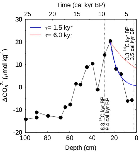
Fig. 3. Reconstructed changes in deep Pacific CO2₃−concentrations after measurements of Marchitto et al. (2005). Vertical lines corre-spond to age control points to which the time scale was adjusted to. The original radiocarbon ages were transformed into calendar ages using INTCAL04 (Reimer et al., 2004). Relaxation of CO2₃− anomalies based onN=N0·e−t /τ withτ=1.5 or 6.0 kyr.

iron limitation) is negligible and other iron proxies such as dust fluxes or concentrations (EPICA-community-members, 2004) which were used previously lead to similar simulation results.

Terrestrial biosphere: The changing terrestrial carbon storage depends on the internally calculated CO2 concen-tration (CO2 fertilisation) and average global temperature, the latter calculated as 3:1 mixture of northern and southern hemispheric temperature with glacial/interglacial amplitudes of 8 and 4 K, respectively (e.g. Kutzbach et al., 1998). Temperature changes were forced by simulation results from Bintanja et al. (2005) for the North, who calculated the av-erage northern (40–80◦_{N) hemispheric temperature changes}

as a function of sea level variations and thus northern land ice sheet distribution based on the stacked benthicδ18O record of Lisiecki and Raymo (2005) (Fig. 2e), and by EPICA Dome C δD for the South (Fig. 2h). Glacial/interglacial fluctuations in terrestrial carbon is with 400−500 PgC well in the range predicted by various modelling and data based studies (see review in K¨ohler and Fischer, 2004). Alternative larger glacial/interglacial changes in terrestrial carbon storage are investigated in a sensitivity study.

CaCO3 chemistry: All changes in the carbon cycle alter [CO2₃−] in the deep ocean. As a consequence the saturation horizon of CaCO3 varies, which then induces changes in either the dissolution or sedimentation rates until a new equilibrium is established and the previous deep ocean [CO2₃−] is obtained again. This process is known as carbon-ate compensation (Broecker and Peng, 1987). In the absence of a sediment model of early diagenesis, which would cover these processes, we here calculated sediment/deep ocean fluxes of calcium carbonate (changing deep ocean DIC and alkalinity in a ratio of 1:2) by the application of an additional boundary condition. All anomalies in deep ocean [CO2₃−] from its preindustrial steady state reference values produce CaCO3 fluxes between sediment and deep ocean to coun-terbalance these anomalies. This sedimentation/dissolution of calcite reacts not instantaneously to the changes in [CO2₃−]. Their time delayed response to bring [CO2₃−] back to its initial value can be approximated by an e-folding timeτ, which is so far not determined accurately. While modelling studies (Archer et al., 1997, 1998) suggest aτ of approximately 6 kyr, an e-folding time calculated from the paleo reconstruction of deep Pacific variability in [CO2₃−] (Marchitto et al., 2005) covering the last glacial/interglacial transition is of the order of 1.5 kyr (Fig. 3). We therefore show simulations with different τ: In the scenario S0.0K carbonate compensation responses instantaneously (τ=1 yr), the sedimentary response is significantly delayed in the scenarios S1.5K (τ=1.5 kyr) and S6.0K (τ=6.0 kyr). This approach covers changes in the net fluxes of DIC and alkalinity, and thus implicitly includes riverine inputs of bicarbonate through weathering (Munhoven, 2002), however, there potential temporal variability is not covered here and might be an area for future improvements.

3 Results

In the following the results of simulated atmospheric CO2 with different response time of the carbonate compensa-tion (scenarios S0.0K, S1.5K, S6.0K) are analysed first (Sect. 3.1), followed by a closer look onto the CaCO3 chem-istry (Sect. 3.2), before we deepen the understanding of our model with a broad sensitivity analysis (Sect. 3.3).

800

700

600

180

200

220

240

260

280

300

C

O

(ppmv)

S6.0k

S1.5k

S0.0k

800

700

600

180

200

220

240

260

280

300

C

O

(ppmv)

(a)

VII

"VIII"

17

600

500

400

180

200

220

240

260

280

300

C

O

(ppmv)

600

500

400

180

200

220

240

260

280

300

C

O

(ppmv)

(b)

V

VI

11

13

15

400

300

200

180

200

220

240

260

280

300

C

O

(ppmv)

400

300

200

180

200

220

240

260

280

300

C

O

(ppmv)

(c)

III

IV

7

9

200

100

0

Time (kyr BP)

180

200

220

240

260

280

300

C

O

(ppmv)

200

100

0

Time (kyr BP)

180

200

220

240

260

280

300

C

O

(ppmv)

(d)

I

II

1

5

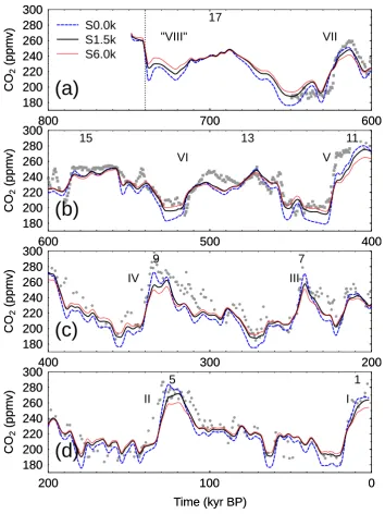
Fig. 4. A detailed view on atmospheric CO2. (a): 740 to 600 kyr BP. (b): 600 to 400 kyr BP. (c): 400 to 200 kyr BP. (d): 200 to 0 kyr BP.

Comparing three different scenarios which differ in the response time of the carbonate compensation: S0.0K: instantaneous response: S1.5K, S6.0K: response delayed by an e-folding time of 1.5 and 6 kyr, respectively. Vostok (grey circles) and EPICA Dome C (grey squares) CO₂ data for comparison. See Fig. 2j for details. Simulations are shown as 3 kyr running mean, dynamics prior to 740 kyr BP (vertical line) are due to model equilibration. MIS of interglacial periods and Terminations (I to VIII) are labelled.

which is up to 15 ppmv higher than during the instantaneous response assumed in S0.0K. During the last five interglacials all three scenarios differ by about 5−10 ppmv with S0.0K simulating the highest, S6.0K the lowest atmospheric CO2. For reasons of simplicity we concentrate in the following on the scenario with moderateτ (S1.5K) and discuss its results in detail. An in-depth analysis of the causes for the different results of the three scenarios is compiled later-on (Sect. 3.2).

VIII VII

VI

V

IV

III

II

I

Number of Termination

0

10

20

30

40

50

60

70

80

90

100

110

120

130

CO

2

rise

(ppmv)

Vostok and EDC data scenario S1.5K sum of one-at-a-time sum of all-but-one

Vostok

pre-Vostok

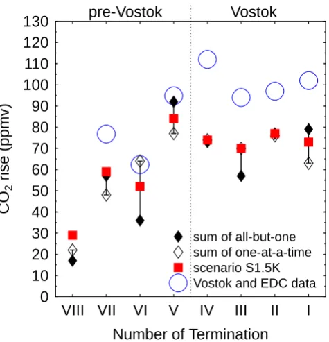
Fig. 5. Estimating the rise in CO2between minima and maxima

across Terminations I to VIII by various methods. Vostok and EPICA Dome C (EDC) CO₂data are compared to scenario S1.5K, and to the summation of the two different single process identifica-tions methods used in Fig. 6 (one-process-at-a-time vs. all-but-one-processes).

Peak values during interglacial periods in MIS 13, 15, and 17 reach∼250 ppmv, with 70 to 120 kyr elapsing in-between. Atmospheric CO2drops during glacials in MIS 12, 14, and 16 to 190–200 ppmv. The agreement of our simulation re-sults with the measurements in terms of timing is especially good during most terminations (I, III, IV, V, VI), but 10 kyr too late (early) at Termination II (VII). However, it has to be kept in mind, that the uncertainty in the age models of the ice cores are still of the order of thousand years (Vostok CO2 data are here used on the orbitally tuned age scale of Shackleton, 2000), and the problem of using different paleo records on their individual age scale might introduce cross dating uncertainties into our results. Accordingly significant differences in timing are not surprising.

The glacial/interglacial amplitudes in CO2across the last five terminations vary between 70 and 85 ppmv in simula-tion S1.5K (Fig. 5). This is on average 20−30 ppmv smaller than in the ice core data, with the best and worst agreements for Termination V (1≈10 ppmv) and IV (1≈40 ppmv), re-spectively. The offset between simulations and data is mainly caused by smaller interglacial values in S1.5K. Some peaks in the CO2data are represented by single points (e.g. LGM, MIS 7, 9) and might therefore not be representative. Scenario S1.5K simulates the smallest glacial/interglacial rise in CO2 of 50 ppmv across Termination VI, about two thirds of the

amplitudes simulated across the Terminations I to V; the CO2 amplitude during Termination VII is of average magnitude (Fig. 5). Termination VIII (CO2rise of 30 ppmv in S1.5K, not yet covered by ice core data) has to be taken with caution as EPICA Dome CδD data prior to 740 kyr BP (J. Jouzel et al., unpublished data) reveal that minimum temperatures and thus full glacial conditions in MIS 18 are reached in even older times. The tendency of cooler interglacials as seen in the EPICA Dome CδD data (EPICA-community-members, 2004) is also mirrored by the measured and simulated CO2 records. The CO2concentration in the pVostok period re-mained longer at relatively high levels, but with smaller CO2 during interglacials and thus smaller glacial/interglacial am-plitudes compared to the Vostok period.

Some major features seen in the CO2 records, however, are not found in the simulations:

(A) The timing in the simulation of CO2reductions during some glaciations is incorrect. This might be caused by an ear-lier decrease in the Antarctic ice core temperature proxiesδD than in the Southern Ocean sea surface temperature (SST). From the deuterium excess record in the ice (Vimeux et al., 2002) it is known that the temperature change in the source regions of the precipitated moisture lags Antarctic tempera-ture during glaciations.

(B) We fail to simulate the CO2maxima above 280 ppmv in the last four interglacials (MIS 1, 5, 7, 9). As our model is driven by various paleo-climatic archives plotted on their in-dividual age scales and of low temporal resolution (∼1 kyr) especially the simulation of peak values in CO2 depends on the temporal matching of these driving records. There-fore, our results here have to be understood as an estimate of low frequency fluctuations in CO2. Furthermore, coral reef growth which increases CO2during sea level high stands (Vecsei and Berger, 2004) is not considered so far leaving space for interpretation during interglacial times in which sea level rose above 70 m below present and the main shelfs were flooded.

(C) CO2rises steep (70 ppmv within 10 kyr) across Termina-tion V into MIS 11 at∼420 kyr BP in the EPICA Dome C data. In the simulation the steep increase is restricted to 45 ppmv followed by a slower rise to full interglacial CO2. This is partially again mirroring the dynamic of the Antarc-tic temperature proxy, which shows a slower relative rise than CO2during the second half of Termination V (Fig. 2h, j). But this is also caused by the timing of the switch from glacial Atlantic THC to its interglacial strength, a process which is responsible for 15 ppmv of the CO2 increase (Fig. 6). This latter process depends on the North Atlantic temperature proxy whose relative timing in respect to the paleo-climatic changes recorded in the Antarctic ice cores might be incor-rect.

P. K¨ohler and H. Fischer: Simulating atmospheric CO2during the last 740 kyr 65

VIII VII VI V IV III II I

Number of Termination -30

-20 -10 0 10 20 30 40 50 60

C

o

n

tr

ib

u

ti

o

n

to

C

O2

ri

s

e

(p

p

m

v

)

Sea ice Sea level

Ocean temperature

Vostok pre-Vostok

Physics (without circulation)

VIII VII VI V IV III II I

Number of Termination

SO vertical mixing NADW formation

Vostok pre-Vostok

Ocean circulation

VIII VII VI V IV III II I

Number of Termination

CaCO3chemistry

Terrestrial biosphere Fe fertilisation

Vostok pre-Vostok

Biogeochemistry

Fig. 6. Impact of different processes on glacial/interglacial changes in CO2during the last eight terminations. We estimate single process

contributions by either the time-dependent forcing of one process only (open symbols), or by calculating the differences between simulation S1.5K and the simulation which excludes the time-dependent forcing of the process in question (filled symbols). Shown here are the contributions to the CO2 rise between minima and maxima crossing Terminations I to VIII. Full time-dependent results underlying our

analysis here are found in Fig. 7 and Fig. 8. The processes are sub-grouped into physics (excluding ocean circulation), ocean circulation, and biogeochemistry and include changes in ocean temperature, sea level, gas-exchange through sea ice, NADW formation, Southern Ocean vertical mixing, iron (Fe) fertilisation of marine biology in the Southern Ocean, terrestrial biosphere, and DIC and alkalinity fluxes between deep ocean and sediment (CaCO3chemistry). Differences between filled and open symbols highlight the high non-linearity of the system.

CaCO3chemistry (carbonate compensation) is a response process to all other changes in the carbon cycle and cannot be analysed as single

effect. The terrestrial carbon storage in the one-at-a-time approach underestimates the effect of CO2fertilisation.

www.climate-of-the-past.net/cp/0000/0001/ Climate of the Past, 0000, 0001–29, 2006

Fig. 6. Impact of different processes on glacial/interglacial changes in CO2during the last eight terminations. We estimate single process

contributions by either the time-dependent forcing of one process only (open symbols), or by calculating the differences between simulation S1.5K and the simulation which excludes the time-dependent forcing of the process in question (filled symbols). Shown here are the contributions to the CO2rise between minima and maxima crossing Terminations I to VIII. Full time-dependent results underlying our

analysis here are found in Fig. 7 and Fig. 8. The processes are sub-grouped into physics (excluding ocean circulation), ocean circulation, and biogeochemistry and include changes in ocean temperature, sea level, gas-exchange through sea ice, NADW formation, Southern Ocean vertical mixing, iron (Fe) fertilisation of marine biology in the Southern Ocean, terrestrial biosphere, and DIC and alkalinity fluxes between deep ocean and sediment (CaCO3chemistry). Differences between filled and open symbols highlight the high non-linearity of the system.

CaCO₃chemistry (carbonate compensation) is a response process to all other changes in the carbon cycle and cannot be analysed as single effect. The terrestrial carbon storage in the one-at-a-time approach underestimates the effect of CO2fertilisation.

accurate and higher resolved record of EPICA Dome CδD (J. Jouzel et al., unpublished data) for the earlier parts of the ice core record is taken to force the model. The uncertainty in the age model in this time period (Brook, 2005) might also be responsible for parts of the offset.

As mentioned by Brook (2005) the EDC2 age model (Schwander et al., 2001) which has been used for all EPICA Dome C records here, might need a revision in the times cov-ering MIS 13 to 15. Our simulations point in the same direc-tion: In general, sea level maxima occur during warm in-terglacial periods, while sea level minima fall together with minimum temperatures. This is the case for the sea level reconstruction based on benthicδ18O data (Bintanja et al., 2005) and δD from EPICA Dome C for the last 450 kyr (Fig. 2). During MIS 13 to 15 these two records are out of phase, which is probably caused by chronological uncertain-ties in the EPICA Dome C records caused by anomalies in ice flow. An updated chronology correcting for these mis-matches is currently developed (F. Parrenin et al., unpub-lished manuscript). The implication of this chronological artefact in the Dome C data sets is, that our reconstruction of CO2 across Termination VI is biased. For example, the contribution from sea level rise during Termination VI is pos-itive, opposing its signal during all other glacial/interglacial transitions (Fig. 6).

In two sensitivity analyses the importance of individual processes were investigated by (a) forcing only one process at a time (Fig. 7) and (b) excluding one process from time-dependent forcings (Fig. 8). From these analyses we estimate the contributions of individual processes to the rise in CO2 during the last eight terminations (Fig. 6) keeping in mind the limited validity of the absolute values due to the high non-linearities of the simulated system. In the second approach (simulating all but one processes simultaneously) the process contributions contain also the amplification of the carbonate compensation. Carbonate compensation itself is only a re-sponse process to all other changes in the carbon cycle and cannot be analysed in the one-at-a-time approach. Carbon storage on land is a function of atmospheric CO2through the CO2 fertilisation of photosynthesis. The one-at-a-time ap-proach, therefore, depict only changes in the terrestrial car-bon pools caused by changes in global temperature, but not by those of the CO2 concentration. For most processes the two approaches agree within 5 ppmv, only the contribution of the terrestrial carbon pools (12 ppmv) and of the ocean temperature (21 ppmv) have higher uncertainties (Fig. 6).

240 260 280 TEMP

240 260 280 SEAL

240 260 280 SICE

240 260 280

CO

2

(ppmv)

NADW

240 260 280 SOX

240 260 280 FE

700 600 500 400 300 200 100 0 Time (kyr BP)

240 260 280 TB

Fig. 7. Analysis of the effect of single processes on atmospheric

CO2. One process at a time was forced externally while all other

forcings were held constant at preindustrial level. Considered processes depict changes in ocean temperature (TEMP), sea level (SEAL), sea ice (SICE), NADW formation (NADW), Southern Ocean vertical mixing (SOX), iron fertilisation in Southern Ocean (FE), carbon storage in terrestrial biosphere (TB). Additionally, a scenario with variable NADW formation including its shut-down during Heinrich events is shown (dashed in sub-figure NADW). In TB the effect of CO2 fertilisation is underestimated due to only

small variability in CO2. Carbonate compensation is a response

process to all other changes in the carbon cycle and cannot be anal-ysed as single effect. All simulation results are shown as 3 kyr run-ning mean.

earlier (36/22 ppmv)), ocean temperature (26/11 ppmv), iron fertilisation in the Southern Ocean (20/14 ppmv), the car-bonate compensation (15/7 ppmv), and NADW formation (13/0 ppmv). Changes in gas exchange caused by sea ice cover (−8/−7 ppmv), sea level (−12/−4 ppmv), and terres-trial carbon storage (−13/−6 ppmv) were processes enlarg-ing the observed CO2rise by up to 33 ppmv during termina-tions. While most processes are reduced in their magnitude

prior to Termination V, the absolute contribution of iron fer-tilisation changes only slightly. Thus, the relative importance of biogeochemical processes is enhanced from∼30% (Ter-mination I−V) to∼40% during earlier terminations. Ocean circulation contributes about 60% during all terminations to the CO2 rise while the contributions of other physical pro-cesses (SST, sea level, sea ice) is less than 10% during Termi-nations I−V and on average neutral earlier (Fig. 6). Accord-ing to our model the smaller interglacial CO2 values in the pre-Vostok period prior to Termination V are mainly caused by smaller interglacial Southern Ocean SST and an Atlantic THC which stayed before MIS 11 in its weaker glacial circu-lation mode.

3.2 A closer look onto the CaCO3chemistry

A deeper understanding of the differences in the three scenar-ios with variable e-folding time of the sedimentary response is obtained by a closer look onto the simulated [CO2₃−] in the deep Pacific Ocean and the total carbon content of the simu-lated system (Fig. 9). We additionally compare these results with the scenario without carbonate compensation (S−CA) and expected changes in [CO2₃−] during the past 150 kyr based on the conceptual understanding of the carbonate com-pensation (Marchitto et al., 2005). For the latter case details and timing have to be taken with caution.

The instantaneous responding sediments (S0.0K) preserve a constant [CO2₃−] of 63µmol kg−1(Fig. 9a). This constancy is paid for by large fluctuations in the total carbon content (Fig. 9b). Total C is up to 1000 PgC larger during glacial pe-riods, which is about 2/3 of the amount of dissolvable CaCO3 for modern times (1600 PgC) (Archer, 1996) In the other ex-treme case of no CaCO3chemistry (S−CA) total C is pre-served, but the [CO2₃−] of the deep Pacific ocean drops during full glacial conditions by almost 25 mmol kg. Both scenarios with reasonable e-folding time of the carbonate compensa-tion lead to variability in total C and deep Pacific [CO2₃−] somewhere between those of the extreme cases: [CO2₃−] varies up to 10 and 14µmol kg−1 around the preindustrial value in S1.5K and S6.0K, respectively. The variability in to-tal C is restricted to 700 PgC (S1.5K) and less than 350 PgC (S6.0K), which is about 2/3 and 1/3 of the variability during instantaneous response. The total C att=0 kyr BP is still 50, 100, and 400 PgC higher in S0.0K, S1.5K and S6.0K, respec-tively, than during steady state for preindustrial conditions. In other words, in the transient simulations which include the carbonate compensation the carbon content at preindus-trial times differs from observational-based estimates by up to 1%. At the end of the glacial or interglacial periods the simulated system in S1.5K and S6.0K is yet not in equilib-rium due to the delayed sedimentary response.

180 210 240

270 S-TEMP

180 210 240

270 S-SEAL

180 210 240

270 S-SICE

180 210 240 270

CO

2

(ppmv)

S-NADW

180 210 240

270 S-SOX

180 210 240 270 S-FE

180 210 240 270 S-TB

700 600 500 400 300 200 100 0 Time (kyr BP)

180 210 240 270 S-CA 180 210 240

270 S-TEMP

180 210 240

270 S-SEAL

180 210 240

270 S-SICE

180 210 240 270

CO

2

(ppmv)

S-NADW

180 210 240

270 S-SOX

180 210 240 270 S-FE

180 210 240 270 S-TB

700 600 500 400 300 200 100 0 Time (kyr BP)

180 210 240 270 S-CA

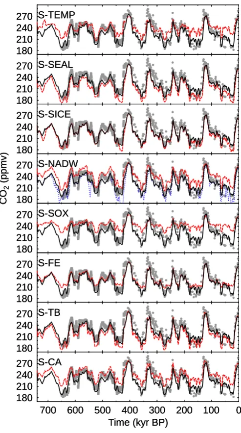
Fig. 8. Analysis of single processes on atmospheric CO2in comparison to the CO2data (grey markers). All processes (scenario S1.5K,

bold black) and all but one process at a time (dash red) were forced externally. Processes depict changes in ocean temperature (S–TEMP), sea level (S–SEAL), sea ice (S–SICE), NADW formation (S–NADW), Southern Ocean vertical mixing (S–SOX), iron fertilisation in the Southern Ocean (S–FE), carbon storage in terrestrial biosphere (S–TB), carbonate compensation (S–CA). Additionally, a scenario with all processes at work and a complete shut-down of NADW formation during all Heinrich events as indicated by IRD in the North Atlantic was simulated (short-dash blue in sub-figure S–NADW), As the inclusion of exchange fluxes between sediment and ocean is converting our modelled carbon cycle to an open system in which total carbon and alkalinity are not conserved anymore a direct comparison between individual simulations becomes difficult due to variations in the overall budgets. All simulation results are shown as 3 kyr running mean.

terminations, drop during glaciations) of up to 30µmol kg−1 caused by other processes, which are followed by a re-laxation over the following several millenia (Broecker and Peng, 1987). An initial rise in [CO2₃−] during terminations is caused by the extraction of DIC from the deep waters by any of the other processes operating on the global car-bon cycle. This increases the pH of the deep ocean which than moves the equilibrium between [CO2], [HCO−₃], and

40 50 60 70 80 90

CO

3

2

- (

mol

kg

-1 )

conceptual after Marchitto et al. (2005)

S6.0K S1.5K S0.0K S-CA

(a)

Pacific

40.0 40.5 41.0 41.5 42.0

T

otal

C

(10

3 PgC)

(b)

Total Carbon

700 600 500 400 300 200 100 0

Time (kyr BP)

160 180 200 220 240 260 280 300

CO

2

(ppmv)

700 600 500 400 300 200 100 0

Time (kyr BP)

160 180 200 220 240 260 280

CO

2

(ppmv)

(c)

Atmosphere

Fig. 9. Carbonate compensation mechanism. Besides the scenarios with different e-folding time of the carbonate compensation (S0.0K,

S1.5K, S6.0K) a scenario without CaCO3chemistry (S–CA) is shown. Conceptual changes in the deep Pacific CO2₃−concentration expected

from measurements (Marchitto et al., 2005) and the understanding of the CaCO₃compensation are also shown in (a). (a) CO2₃−concentration in the deep Indo-Pacific ocean box. (b) Total carbon of the simulated ocean/atmosphere/biosphere system. (c) Atmospheric CO2. CO2data

as described in Fig. 2 as grey markers. All simulation results are shown as 3 kyr running mean.

saturation horizon towards deeper waters) or increased dis-solution (if [CO2₃−] is decreased which shifts the calcite sat-uration horizon towards shallower waters) of CaCO3. Re-cent measurements on three cores in the equatorial Pacific (Marchitto et al., 2005) support this dynamic, the change in [CO2₃−] is of the order of 25–30µmol kg−1, although the gradients at the beginning of individual events are not as steep as theoretically predicted and the sedimentary response seems to be faster than concluded from process-based mod-els (Fig. 3).

All-together, this means, that a rise in surface waters [CO2] (similar to a rise in atmospheric CO2) implies also the extraction of carbon from the deep ocean. This extraction causes increased sedimentation, which is another loss term of carbon. However, due to the ratio of alkalinity:DIC=2:1 in all carbonate fluxes the overall effect of sedimentation is a pH reduction in the deep ocean which again shifts the car-bonate system from [CO2₃−] towards [CO2], leading finally

to a further rise in surface [CO2]. Thus, carbonate compen-sation is a positive feedback. It always acts as an amplifier to ongoing processes operating on the global carbon cycle.

For this interpretation it has to be kept in mind, that the riverine input of bicarbonate was not explicit formulated, and therefore not allowed to vary over time. Improving this short-coming together with the use of a process-based sediment model might substanitally alter our current understanding of the importance of the CaCO3chemistry for atmospheric CO2.

estimate. A time-delayed response of the CaCO3chemistry reduces this contribution by a factor of two. An ocean car-bon cycle model with higher vertical resolution together with a process-based sediment module are needed for a refined quantification of this number.

3.3 Model sensitivity

In the following subsection we will investigate the sensitiv-ity of BICYCLE by the variation of the glacial/interglacial amplitudes of all processes and analyse specific parts of our model in greater detail. These parts (sea ice, ocean circula-tion, marine biota, terrestrial biosphere) need some in-depth analysis due to the simplicity in which they are embedded in our model.

3.3.1 Variation of the glacial/interglacial strength of indi-vidual processes

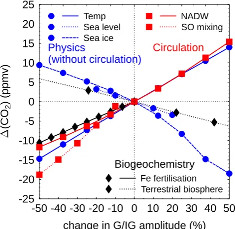
We investigated the sensitivity of our model to the am-plitudes in the different processes contributing to the glacial/interglacial CO2 rise. We therefore varied their glacial/interglacial amplitudes by up to ±50% from their standards and compared the relative impacts on CO2for Ter-mination I (Fig. 10). The sensitivity of the simulated CO2 to changes in the amplitude of one process is rather linear. Varying the amplitude of a single process by less than 20% would result in less than∼7 ppmv deviation in CO2. We therefore evaluate our model as rather robust to the detailed knowledge of individual processes. This, however, neglects nonlinear effects from combined changes for alternative sce-narios in which more than one process is operating with a different glacial/interglacial amplitude.

3.3.2 Sea ice

Our approach proposes a decline of CO2by∼10 ppmv dur-ing terminations contributed by changes in the gas exchange rate through the shrinking of sea ice coverage. This would contradict a previous modelling study (Stephens and Keel-ing, 2000) which concluded that a nearly full sea ice coverage of the Southern Ocean south of 55◦S would reduce CO2by 67 ppmv. Although the reliability of this previous study was questioned because of the proposed very high sea ice cov-erage (Morales-Maqueda and Rahmstorf, 2001) the question remains why our model responses in the opposite direction. It was shown (Archer et al., 2003) that a model response to a fully Southern Ocean sea ice coverage is especially highly model dependent.

In our study the decline in CO2 during deglaciations is caused by larger gas exchange rate in the North Atlantic Ocean which itself is caused by the decrease in the north-ern sea ice cover. The preindustrial North Atlantic is a sink for CO2while the Southern Ocean is a source, both in our model and if recent gas exchange estimates are corrected for anthropogenic CO2 (Takahashi et al., 2002; McNeil et al.,

-50 -40 -30 -20 -10 0 10 20 30 40 50

change in G/IG amplitude (%)

-25

-20

-15

-10

-5

0

5

10

15

20

25

(C

O

)

(ppmv)

Terrestrial biosphere Fe fertilisation Sea ice

Sea level Temp

SO mixing NADW

Biogeochemistry

Circulation

Physics

(without circulation)

Fig. 10. Sensitivity analysis of the impact of the glacial/interglacial

amplitudes of the individual processes on the rise in atmospheric CO2during the last glacial/interglacial transition covering

Termi-nation I (30–0 kyr). The figure shows the differences in the rise in CO2between scenarios (all processes included) with variable

am-plitude in one process and scenario S1.5K. Processes depict changes in ocean temperature (Temp), sea level, gas-exchange rate through sea ice, NADW formation, Southern Ocean vertical mixing, Fe fer-tilisation in the Southern Ocean, and carbon storage in terrestrial biosphere. Note, that the carbonate compensation is a response pro-cess and cannot be modified in its amplitude. Glacial/interglacial amplitude of sea level change was varied only±20% due to high reliability of known sea level change. The glacial/interglacial am-plitudes of iron (Fe) fertilisation, and Southern Ocean vertical mix-ing (Southern Ocean mixmix-ing) could only be reduced as they were operating on their possible upper limit.

2006). Therefore, reducing gas exchange during glacials in the North is increasing the glacial atmospheric CO2. The net effect of sea ice coverage in the Southern Ocean is negligi-ble and reaches the magnitude of the North only when the Southern Ocean surface box is nearly fully covered by sea ice (Fig. 11). However, our data based assumption proposes only an average annual glacial sea ice coverage of 30% in our Southern Ocean surface box.

700 600 500 400 300 200 100 0 Time (kyr BP)

250 260 270 280

CO

2

(ppmv)

S only (90% coverage) S only (60% coverage) S only (30% coverage) N and S

Fig. 11. Northern and southern contributions to the impact of sea

ice cover on atmospheric CO2in a single processes analysis. In

the reference run (N and S) nearly no contribution comes from the Southern Ocean sea ice, which covers 30% of the Southern Ocean surface box area during LGM. Increasing this Southern Ocean sea ice areal cover up to 90% coverage shows opposing trends (reduced CO2during glacial times) from the northern contribution (increased

CO₂ during glacial times). This Southern Ocean behaviour is in line with previous investigations (Stephens and Keeling, 2000). All simulation results are shown as 3 kyr running mean.

3.3.3 Ocean circulation

In our reference scenario we have chosen to keep NADW formation unchanged during Heinrich events as there are ev-idences from productivity (Sachs and Anderson, 2005) and sea level (Siddall et al., 2003) reconstructions, that the impact may differ. Here, we estimate the maximum impact through a complete shut-down of NADW formation during Heinrich events identified by ice rafted debris (IRD) in the North At-lantic sediment record ODP980 measured on the same core than two other paleo records used already in our study (North Atlantic SST and benthic δ18O) (McManus et al., 1999; Wright and Flower, 2002). IRD in percentage of sediment grains larger than 150µm (relative IRD) is a proxy for the occurrence of Heinrich events (Heinrich, 1988). We used the relative strength IRDH=10% as threshold indicating large iceberg and thus freshwater discharges occurring in the North Atlantic which result in a complete shut-down of the NADW formation during glacial times in our model. This threshold was derived from the analysis of IRD and known Heinrich events during the last glacial cycle (Heinrich, 1988). During two time intervals relative IRD data were missing in ODP980 (740–700 and 543–500 kyr BP). The absolute IRD record (lithics/g) spanned our whole simulation period (Wright and Flower, 2002) and showed no major excursions in the in-complete periods of the relative IRD record apart from one large peak during the period 740–700 kyr BP. However, this absolute record is unsuitable for the predictions of Heinrich events as known events occurring during the last glacial cycle (Heinrich, 1988) would have been overestimated. IRD in a second core approximately 1000 km apart (ODP984) shows

similar features during 500–740 kyr BP (Wright and Flower, 2002) suggesting an at least regional distribution of the IRD signals measured in ODP980 and the changes in freshwater discharge indicated by them.

A shut-down of the NADW formation occurring during the Heinrich events, which were identified by the relative IRD record, reduces atmospheric CO2during glacial climate conditions by about 10−20 ppmv (Fig. 8). Only a Heinrich event around 550 kyr BP happening during intermediate cli-mate conditions and those events in the glacial maximum proceeding Termination V (420 kyr BP) lead to drops in CO2 by 30−40 ppmv. The selection criteria for Heinrich events (IRDH=10%) was varied in a sensitivity study (Fig. 12b), and showed rather unchanged response of CO2for a thresh-old increase by a factor of two, and an extension of Heinrich events if IRDHwas lowered.

The impacts of the thresholdδ18ONADWin ODP980 which indicates a switch from glacial to interglacial circulation pat-terns in the Atlantic Ocean (strength of NADW formation) was also tested. During interglacial times this strength in NADW depends to a certain extent on the chosen threshold (Fig. 12a). During warm periods around 200, 570, 610, and 690 kyr BP the Atlantic THC is only switching into its inter-glacial mode (16 Sv of NADW formation) and leads to a rise in CO2by about 10 ppmv, when the thresholdδ18ONADWis increased. This implies that in our standard scenarios the NADW stayed in its glacial mode during these times. In other words, the Atlantic THC stayed constant over time in its glacial mode before MIS 11 (740−420 kyr BP) and would switch only to its interglacial mode in the pre-Vostok period if a slightly colder temperature threshold is assumed (higher

δ18ONADW) than in the standard case.

180

200

220

240

260

280

CO

2

(ppmv)

3.2 3.0 2.8 2.6 2.4

(a) NADW

180

200

220

240

260

280

CO

2

(ppmv)

off 20 15 10 5

(b) NADW in H events

700

600

500

400

300

200

100

0

Time (kyr BP)

180

200

220

240

260

280

CO

2

(ppmv)

71 5

138 271

205

(c) Fe fert.

180

200

220

240

260

280

CO

2

(ppmv)

180

200

220

240

260

280

CO

2

(ppmv)

700

600

500

400

300

200

100

0

Time (kyr BP)

180

200

220

240

260

280

CO

2

(ppmv)

Fig. 12. Variation of fixed threshold values used during simulations. Simulation results were shown as 3 kyr running mean. Bold depicts

always the standard simulation S1.5K using the standard values, data (grey markers) as described in Fig. 2. (a): Varying the threshold

δ18ONADWin ODP980 which indicates changes in the strength in the NADW formation (δ18ONADW=2.4,2.6,2.8,3.0,3.2‰). (b): Varying

the threshold in IRD as the indicator for Heinrich events measured in ODP980 (IRDH=5,10,15,20%). Note, that in our standard scenario

the NADW formation during identified Heinrich events is not shut-down. (c): Varying the threshold in the atmospheric iron flux as measured in EPICA Dome C which is a proxy for the onset of iron fertilisation in the Southern Ocean (FeMB=5,71,138,205,271µg m−2yr−1).

temperature anomalies during Heinrich events would also impact on the terrestrial carbon cycle (K¨ohler et al., 2005b). During cold periods the treeline in Eurasia would shift south-wards, and soil respiration would decrease. In BICYCLEthe nutrient distribution is also affected by a change in ocean cir-culation. But only a reduction in the NADW formation below the glacial strength of 10 Sv causes a decrease in the marine export production due to macro-nutrient depletion and causes a rise in atmospheric CO2. This change in the marine biota is in line with other studies (Schmittner, 2005). A more detailed investigation of the NADW strength and CO2in BICYCLEis found in K¨ohler et al. (2006).

3.3.4 Marine biota

200

220

240

260

280

300

CO

2

(ppmv)

(a)

180

200

220

240

260

280

300

CO

2

(ppmv)

1000

1200

1400

1600

1800

2000

2200

T

erre

strial

C

(PgC)

(b)

700

600

500

400

300

200

100

0

Time (kyr BP)

40.0

40.5

41.0

41.5

42.0

T

otal

C

(10

3

PgC)

S6.0k S1.5k S0.0k

S6.0kTB+ S1.5kTB+ S0.0kTB+

(c)

Fig. 13. Additionally to the simulation S0.0K, S1.5K, S6.0K an alternative pathway of terrestrial biosphere regrowth was considered with

greater climate and CO₂dependency leading to higher glacial/interglacial amplitudes in the terrestrial carbon stocks (S0.0KTB+, S1.5KTB+, S6.0KTB+). Different e-folding time of the calcite compensation as given in the scenario names. (a): Atmospheric CO2, data (grey markers)

as described in Fig. 2. (b): Terrestrial carbon storage. (c): Total carbon storage in the atmosphere/ocean/biosphere system. All simulation results are shown as 3 kyr running mean.

fertilisation experiments. Additional to the data evidences for an enhanced glacial marine biology as reviewed previ-ously (K¨ohler et al., 2005a) new data of extensive phyto-plankton blooms in the Atlantic sector of the glacial Southern Ocean were published recently (Abelmann et al., 2006), giv-ing further support for our assumptions.

The impact of Southern Ocean iron fertilisation on CO2 was also a threshold-dependent process. Changes in sim-ulated CO2 occur for a two fold reduction of the thresh-old during times of high iron flux fluctuations, e.g. around 150−180 kyr BP. Simulated atmospheric CO2varied signif-icantly (>20 ppmv) if the threshold in the EPICA Dome C iron flux on which the marine export production depends is reduced by one order of magnitude (Fig. 12c). This would imply that the marine biota in the Southern Ocean is nearly never iron limited and global export production reduces

at-mospheric CO2 throughout most of the simulation period. The threshold approach neglects details in the dynamics of the different iron proxies for full glacial conditions and is partly responsible for the similar responses of our model to the use of the three different iron proxies.

3.3.5 Terrestrial biosphere

the sensitivity of the terrestrial module on climate and CO2 is the same within the two sets of experiments. The exist-ing difference in the amplitudes within a set of simulations is caused by the internal feedback of the CO2dependent terres-trial NPP (CO2fertilisation). The change in the amplitude in terrestrial carbon storage leads also to different CaCO3fluxes between sediment and deep ocean and thus to different fluc-tuations in the overall carbon budget. While the change in the total carbon of the simulated ocean/atmosphere/biosphere system is 1000, 700, and 350 PgC in S0.0K, S1.5K and S6.0K, respectively, this amplitude is increased to 1700, 1000, and 500 PgC in S0.0KTB+, S1.5KTB+ and S6.0KTB+ (Fig. 13c). In S1.5KTB+ and S6.0KTB+ the total C con-tent att=0 kyr BP is 250 and 500 PgC higher than in steady state simulations for this climate period. This offset in the to-tal C budget between transient simulations and preindustrial steady state makes the upper end of the proposed range in the variation of the terrestrial carbon content very unlikely. As overall effect glacial atmospheric CO2is about 15 ppmv higher in the STB+ scenarios than in the corresponding sim-ulations with lower terrestrial variability (Fig. 13a).

4 Discussion and conclusions

In this study we simulate low frequency changes in the car-bon cycle during the late Pleistocene. Our standard scenar-ios match observed atmospheric CO2during the last 650 kyr rather well (r2∼0.75). The novelty of our approach is the fact that our interpretation how the global carbon cycle in-cluding its isotopes is operating during Termination I seems to be sufficient to interpret the variations in atmospheric CO2 not only during the regular variations observed in the Vos-tok ice core but also to simulate smaller glacial/interglacial amplitudes prior to Termination V. The application of our model on these long timescales is a confirmation that our as-sumptions made for and our interpretation gained from the simulation of the carbon cycle during Termination I (K¨ohler et al., 2005a) are not restricted to this very narrow time win-dow, but are of general nature. The time-delayed response of the carbonate compensation is an important detail of the CaCO3chemistry which was not considered in earlier appli-cations of this model. The e-folding timeτ of the relaxation of any perturbation of the deep ocean [CO2₃−] estimated from data and models is still large, however, the consequences are even with a moderate response time (τ=1.5 kyr) that the car-bon cycle in our model never reaches an equilibrium within the last 740 kyr; the total carbon budget is constantly varying due to sedimentation or dissolution. Carbonate compensa-tion with moderate response time (1.5 kyr) contributes about 15 ppmv to the rise of CO2during the last five terminations. This is of the order suggested by Joos et al. (2004) during the Holocene as a consequence of the reorganisation of the car-bon cycle over Termination I. It is about half of the amount suggested by our previous study (K¨ohler et al., 2005a), in

which we alternatively prescribed the changes in the lyso-cline as additional boundary condition. These lysolyso-cline vari-ations, however, are less well known over the whole 740 kyr period for the different ocean basins (Farrell and Prell, 1989) and the interpretation of available data is highly discussed (Archer, 1991). The previous approach of a variable lyso-cline leads to results similar to those of the scenario with instantaneously responding sediments (S0.0K). The missing response time in this approach was therefore a reason to re-vise and update our model here.

The missing temporal variability of the riverine input of bi-carbonate and its subsequent response by the bi-carbonate com-pensation might be one of the main simplifications of our study. The input of HCO−₃ through rivers is estimated to vary on glacial/interglacial timescale by about 25% (Jones et al., 2002; Munhoven, 2002). This reduced interglacial riverine input leads to a rise of atmospheric CO2 of the or-der of 10 ppmv, however, uncertainties in both the variability of the input fluxes itself and the response of the carbon cycle are with about 100% large.

There are several hypothesis on possible changes in the carbon cycle found in the literature, which we did not follow up here for various reasons, because they are either too com-plex to be followed in detail with our model (silicic acid leak-age hypothesis), because of recent evidences arguing against them (rain ratio hypothesis), or because we expect only small contributions to the change in CO2(North Pacific biology). They are discussed in greater detail in K¨ohler et al. (2005a). The potential of a change in the rain ratio of organic to inor-ganic marine export production, for example, is one theory (Archer and Maier-Reimer, 1994; Klaas and Archer, 2002; Ridgwell, 2003a), whose impact on CO2 is limited to less than 15 ppmv in BICYCLE. The silicic acid leakage hypothe-sis (Brzezinski et al., 2002; Matsumoto et al., 2002) involves shifts in phytoplankton communities and operates via a com-bination of iron fertilisation in the Southern Ocean and lo-cal changes in the the rain ratio. Other HNLC regions of the world ocean apart from the Southern Ocean have also the potential for an enhanced glacial export production, although with less capacity for atmospheric CO2. One of these promi-nent regions is the North Pacific where a higher glacial export production might result in a decrease in CO2of up to 8 ppmv (R¨othlisberger et al., 2004). A recent interpretation of proxy data (Jaccard et al., 2005) makes this region also a candidate for a highly stratified water column in glacial times. This physical effect might be even more important for CO2 than the change in the biology.

Our results are further supported by reconstructed pH in the equatorial Atlantic surface waters, which are based on

700 600 500 400 300 200 100 0 Time (kyr BP)

8.1 8.15 8.2 8.25 8.3 8.35

pH

S6.0k S1.5k S0.0k

1 5 7 9 11 13 15 17

Fig. 14. Comparison of simulated pH in the equatorial Atlantic

sur-face box with pH reconstruction (circles) based on boron isotopes

δ11B measured in planktic foraminifers (H¨onisch and Hemming, 2005). Simulation results are shown as 3 kyr running mean. Num-bers denote marine isotope stages during interglacial periods.

amplitude of up to 0.15 pH units (scenario S0.0K; less than 0.10 pH units in S1.5K and S6.0K) in this area, although min-ima during interglacial periods are smaller in the data than in the model.

These simulation results are an in-depth description of our contribution to the “EPICA challenge” (Wolff et al., 2004, 2005). The other seven entries to the “EPICA challenge” (Wolff et al., 2005) were either based on a conceptual mod-elling approach (Paillard and Parrenin, 2004) or on differ-ent correlation functions of the two EPICA Dome C records (dust, δD) and others paleo-climatic archives. Thus, they all tested different hypotheses, but were per se unable to validate their hypothesis by the comparison of other vari-ables of the carbon cycle with additional reconstructions. Nevertheless, all other approaches using existing Antarctic temperature proxies and simple regression functions were able to predict CO2with similar high accuracy (Wolff et al., 2005). Can we understand this coupling of atmospheric CO2 and Antarctic/Southern Ocean temperature from our process-based modelling approach? SST of the Southern Ocean it-self (which is a function of EPICA Dome CδD) is accord-ing to our model responsible for half of the rise in CO2 caused by ocean temperature, which would be ∼15 ppmv during Termination I. Changes in sea ice cover and Southern Ocean vertical mixing are in BICYCLEfunctions of South-ern Ocean SST and thus of EPICA Dome C δD, causing 0 ppmv and 35 ppmv, respectively. Furthermore, CaCO3 compensation as amplifying process will contribute about 5−10 ppmv. Summarising, we are able to explain a rise in CO2of 55−60 ppmv during Termination I only by direct and indirect effects of Southern Ocean temperature changes and thus by the evolution of the EPICA Dome CδD record. How-ever, these are incomplete solutions, because other important changes in the carbon cycle are known to have happened, such as changing concentration of DIC due to sea level vari-ations or changing carbon storage on land which would both operate in the opposite direction.

To our knowledge, there exist so far two transient mod-elling approaches which try to explain the variability of at-mospheric CO2during the late Pleistocene both using con-ceptual models (Gildor et al., 2002; Paillard and Parrenin, 2004) and concentrate on changes in ocean physics. These two approaches differ widely, one (Gildor et al., 2002) being purely theoretically and trying to explain the typi-cal amplitude and seesaw shape of CO2 observed in Vos-tok, while the other (Paillard and Parrenin, 2004) is forced by insolation over the last 1000 kyr. However, both pin-point reduced glacial vertical mixing in the Southern Ocean as one mechanism which contributes significantly to the glacial/interglacial rise in CO2. While we here support the importance of changes in Southern Ocean vertical mixing, we also want to point out that especially those processes which modify the overall budgets of DIC and alkalinity in the ocean need consideration (Archer et al., 1997) and a re-stricted view onto the ocean/atmosphere carbonate system only is of limited validity for a complete understanding of the observed changes in the carbon cycle as recorded in the ice cores.

The chosen model design, that Southern Ocean vertical mixing is a function of Southern Ocean temperature and thus of EPICA Dome CδD, might be questioned. It was moti-vated by the observed vertical and temporal gradient inδ13C in the Southern Ocean sediment cores (Hodell et al., 2003). It turns out that this process is the most important one for atmospheric CO2variability. As a consequence this process alone together with its amplification through CaCO3 com-pensation can explain 40 ppmv of the rise in CO2during Ter-mination I. To support this assumption we argued previously (K¨ohler et al., 2005a) with additional evidences from nutri-ent reconstructions (Franc¸ois et al., 1997) and the salinity-driven stratification of the glacial ocean (Adkins et al., 2002). Further support came from the two conceptual models men-tioned earlier (Gildor et al., 2002; Paillard and Parrenin, 2004) and a box model study which investigates the role of Southern Ocean mixing and upwelling on CO2(Watson and Naveira-Garabato, 2006). In the meantime, another physi-cally based hypothesis was added to the scenarios which pro-pose a glacial stratified Southern Ocean. Toggweiler et al. (2006) hypothesised that a northward shift in the westerly winds during glacial climate would prevent wind-driven up-welling in the Southern Ocean. Their carbon cycle response to this change in ocean ventilation is a glacial decrease in atmospheric CO2of 35 ppmv, very similar to our results.

of debate (e.g. Bender, 2003; Friedlingstein et al., 2003). The overall effect of temperature variations on soil carbon storage is not yet resolved (Davidson and Janssens, 2006). The feedback loop of climate, dust and CO2(Ridgwell and Watson, 2002) is another example for the complexity of the system. Laboratory experiments indicate a CO2-dependent calcite production rate of marine calcifiers (Riebesell et al., 2000). These are some examples of the complexity of the carbon cycle-climate system, whose detailed investigation is needed for an in-depth understanding. Nevertheless, from our simple approach here the potentials of various globally important processes can be highlighted, and thus the choice of foci for future investigations is possible.

This box model study provides an interpretation of low fre-quency changes in atmospheric CO2during the past 740 kyr based on a carbon cycle box model forced by various paleo-climatic records forward in time. The potential contributions of important physical and biogeochemical processes to CO2 variability were investigated. As this study is based on a rather simplistic model which highlights also the uncertain-ties embedded within the approach its results should be un-derstood as an invitation to more complex coupled carbon cycle-climate models to be cross-checked as a whole or in specific parts.

Acknowledgements. This study was performed within RESPIC, a

project funded through the German Climate Research Programme DEKLIM (BMBF). R. Bintanja, B. H¨onisch, J. Jouzel, V. Masson-Delmotte, J. McManus and U. Siegenthaler kindly provided data sets. We like to thank the EPICA challenge team for the inspiring scientific quest. Thanks to E. Wolff, V. Brovkin, and the three anonymous referees for their helpful comments on the discussion version of this article. This work is a contribution to the European Project for Ice Coring in Antarctica (EPICA), a joint European Science Foundation/European Commission scientific programme, funded by the EU (EPICA-MIS) and by national contributions from Belgium, Denmark, France, Germany, Italy, the Netherlands, Norway, Sweden, Switzerland and the United Kingdom. The main logistic support was provided by IPEV an