Cycle time reduction by inventory management

Full text

(1)8/17/2019. Master thesis Cycle time reduction by inventory management Public Version. Lars Tijhuis s1540823 Industrial Engineering & Management Production & Logistic Management. Company supervisors: Person Y Person Z. University supervisors: Dr. I. Seyran - Topan Dr. E. Topan.

(2) I.

(3) Colophon Document Master thesis. Version Final report. Title Cycle time reduction by inventory management. Author L.J.B. Tijhuis [email protected]. Educational institution University of Twente Postbus 217 7500 AE Enschede. Faculty Faculty of Behavioural, Management and Social sciences. Study Program MSc Industrial Engineering and Management. Specialisation Production and Logistic Management. Examination Committee University of Twente Dr. I. Seyran – Topan Dr. E. Topan. Company X Person Y Person Z. Date of publication 17-8-2019. Copyright ©L.J.B Tijhuis, the Netherlands All rights reserved. Nothing in this publication may be reproduced, stored or distributed, in any form or in any way, without permission of the author.. II.

(4) III.

(5) Preface This master thesis is part of my graduation project that I executed at Company X. This thesis is the final part of my Master Industrial Engineering and Management at the University of Twente. Within this master, I completed courses of the specialization Production and Logistic Management. Executing this graduation project has been an exciting experience to apply theory in practice. First, I would like to thank my supervisors at Company X, Person Y and Person Z, for their guidance during my graduation project. They gave me the opportunity to conduct my research within their department at Company X. Next to this, they took time and effort to discuss my findings and progress. In addition, I would like to thank all other employees who have given me an enjoyable internship at Company X. Second, my gratitude goes to my first supervisor from the University of Twente, Ipek SeyranTopan. She provided me with constructive feedback and gave me new insights, which improved the quality of my research. Furthermore, I would like to thank Engin Topan for being the second supervisor and providing useful input to improve my report. Lastly, I want to thank my family and friends for their support during my graduation project. Enjoy reading my master thesis! Lars Tijhuis. IV.

(6) Management summary This research is conducted at Company X, which is a leading provider of comprehensive design and manufacturing solutions to customers on a global basis. Company X is a business-tobusiness company, which means that Company X engineers and produces products for other companies. This study focusses on reducing the Integral Cycle Times (ICT) of products of Customer Y, which contains the following type of products: cabinets, spare parts, small boxes and Printed Circuit Board Assemblies. The characteristics of the products and process resulted in the decision to focus on cycle time reduction by inventory management. Therefore, the following research question is developed which has to be answered during this research:. Which inventory policy should be used at Company X to reduce the Integral Cycle Times of the products for Customer Y taking into account financial risks and reliability risks? The answer of this research question is formulated by answering several sub questions during the different chapters in this report. First, Chapter 1 introduces the company and its products to get familiar with it before starting with the research. The chapter described the products involved in this research and which processes are important for this research. Besides, the stakeholders of this research are identified. This will be used in the next phase, where the problem identification is executed and the design of the research is done. Secondly, Chapter 2 elaborates on the problem identification and the design of this research. There is described which research questions are formulated based on the problem identification. In this chapter is explained that a large part of the cycle time is determined by a couple of Stock Keeping Units (SKUs). This resulted in the decision to focus on the application of safety stocks for these SKUs. Thereafter, Chapter 3 is dedicated to analyzing the current situation at Company X. This analysis gives insights in the current cycle times and aspects of inventory management, such as safety stocks and inventory turnover. Besides, the characteristics of the involved products and SKUs are analyzed, which will be used later on in this research. Then, Chapter 4 present the executed literature review to find out which inventory policies can be applied at Company X. These inventory policies consists of finding the reorder point, order quantity and safety stock. This showed us the importance of determining the right order quantities and safety stock levels for SKUs. This literature presented us the formula for the Economic Order Quantity, which optimizes the order quantity while minimizing the resulting order and holding costs. Thereafter, there is investigated how the safety stocks should be calculated to capture uncertainty in demand of the SKUs. The findings of this chapter are applied in the modelling phase to apply the right calculations. In Chapter 5 is the constructed model and corresponding calculations presented. This model is used to determine the right inventory policy parameters for SKUs and analyze the resulting outcome. This analysis is presented in Chapter 6, where the inventory value, annual costs, financial risks and performances are discussed. First, there is investigated which safety stocks are needed to achieve a certain ICT. Therefore, there are distinguished two types of safety stock. The first type of safety stock has to cover V.

(7) the average demand outside the ICT of an SKU. The second type of safety stock has to cover the demand variation outside the ICT of an SKU. Analyzing the relationship between the safety stocks and the obtained ICT showed us that shortening the ICTs results in an exponential increase of the safety stock value. This is caused by the fact that the number of SKUs with safety stock increases and next to this the average demand and demand variation to be covered also increases. Therefore, Company X have to investigate together with the customer what the optimal ICTs and prevent excessive safety stocks. The analysis phase focuses on a scenario of an obtained ICT of 16 weeks for the involved products and the corresponding performances are estimated with the model and compared with the current situation. The required safety stocks to achieve this ICT reduction have a value of € 995,913. Important to note is that 10 SKUs cause more than half of the value of this safety stock. Despite, the value of the safety stock is just 2.3% of the expected annual sales of the products. Applying these safety stocks results in annual holding costs of € 84,852. ICTs of 16 weeks for all involved products results in a ICT reduction of 43.1 %. Next to the analysis of the required safety stocks, the overall performances of the application of inventory management with respect to inventory value is analyzed. The application of the EOQ formula to determine the order quantities has a positive influence on the average cycle inventory. Combining this together with the safety stock to reduce ICT still results in a reduction of the average inventory value of € 939,356. This is 22.1% less than the current inventory value of the SKUs. This results in an improvement of the inventory turnover from 6.7 to 8.6. Another important aspect of inventory management is the resulting annual order and holding costs. The annual order costs are dependent of the number of order per year and the cost per order and the holding costs depend on the average inventory value and holding cost rate. Again the influence of the application of EOQs and safety stocks to reduce the ICT on the annual costs is analyzed. Applying both results in a decrease in ordering and holding costs, which is quantified with an annual saving of € 327,669. Lastly, Chapter 7 elaborates on the resulting conclusions and recommendations of this research. These conclusions and recommendations are based on the findings throughout the whole research. The following three conclusions are formulated: - ICTs can be reduced by applying safety stocks for SKUs with long lead times . - Determining order quantities by using the EOQ formula results in savings on annual order costs and holding costs. - Applying the suggested inventory management results in a reduction of average inventory value and indirectly an increase of the inventory turnover. The following recommendations are formulated for Company X based on this research: - Use the model as starting to point to achieve ICT reduction by inventory management - Purchase SKUs with order quantities based on EOQ, regardless of the ICT reduction of products - Involve Customer Y in the topic of ICT reduction of the products and negotiate about liabilities. VI.

(8) Table of Contents Management summary..............................................................................................................V List of figures .............................................................................................................................. X List of tables ............................................................................................................................. XII List of abbreviations ................................................................................................................ XIII 1. Company profile................................................................................................................. 1. 2. Research design ................................................................................................................. 2. 3. 4. 2.1. Research context ......................................................................................................... 2. 2.2. Research motivation ................................................................................................... 4. 2.3. Problem description .................................................................................................... 4. 2.4. Research objective ...................................................................................................... 5. 2.5. Research questions ..................................................................................................... 6. 2.6. Scope ........................................................................................................................... 7. 2.7. Deliverables ................................................................................................................. 7. Current situation analysis .................................................................................................. 8 3.1. Qualitative analysis ..................................................................................................... 8. 3.2. Lead times of components .......................................................................................... 9. 3.3. Internal assembly times ............................................................................................ 10. 3.4. Safety stock for components .................................................................................... 13. 3.5. Minimum Order Quantity for components............................................................... 16. 3.6. Inventory On Hand .................................................................................................... 16. 3.7. Inventory turnover .................................................................................................... 17. 3.8. Causes of high lead times .......................................................................................... 18. 3.9. Conclusion ................................................................................................................. 19. Literature review.............................................................................................................. 21 4.1. Inventory management ............................................................................................. 21. 4.1.1. Functional classification of inventories ............................................................. 21. 4.1.2. Cycle and safety inventory ................................................................................. 22. 4.2. Inventory control policies ......................................................................................... 23. 4.2.1. Continuous review policies ................................................................................ 23. 4.2.2. Periodic review policies ..................................................................................... 25. 4.3. Item classification...................................................................................................... 26. 4.3.1. ABC analysis ....................................................................................................... 26. 4.3.2. Multi-criteria ABC analysis ................................................................................. 27. 4.3.3. XYZ-analysis ........................................................................................................ 27 VII.

(9) 4.4. Economic Order Quantity (EOQ) ............................................................................... 28. 4.5. Reorder point ............................................................................................................ 29. 4.6. Safety stock ............................................................................................................... 30. 4.7. Application of literature in the research’s context ................................................... 32. 4.7.1. Inventory policy ................................................................................................. 32. 4.7.2. EOQ and safety stock determination ................................................................. 33. 4.8 5. Model construction.......................................................................................................... 35 5.1. Conceptual model ..................................................................................................... 35. 5.1.1. Input ................................................................................................................... 36. 5.1.2. Model ................................................................................................................. 37. 5.1.3. Output ................................................................................................................ 37. 5.2. Inventory policy parameters ..................................................................................... 39. 5.2.1. Order quantities ................................................................................................. 39. 5.2.2. Safety stocks ...................................................................................................... 42. 5.2.3. Reorder points ................................................................................................... 45. 5.3. Output ....................................................................................................................... 46. 5.3.1. Inventory value .................................................................................................. 47. 5.3.2. Annual costs ....................................................................................................... 49. 5.3.3. Financial risks ..................................................................................................... 50. 5.3.4. Performances ..................................................................................................... 53. 5.3.5. Dashboard .......................................................................................................... 55. 5.4 6. Conclusion ................................................................................................................. 34. Conclusion ................................................................................................................. 56. Model analysis ................................................................................................................. 57 6.1. Scope of the analysis ................................................................................................. 57. 6.2. Safety stocks for ICT reduction ................................................................................. 58. 6.2.1. Safety stock to cover average demand .............................................................. 58. 6.2.2. Safety stock to cover demand variation ............................................................ 60. 6.2.3. Total safety stocks value .................................................................................... 62. 6.3. Inventory value.......................................................................................................... 63. 6.3.1. Cycle inventory .................................................................................................. 63. 6.3.2. Safety stock ........................................................................................................ 64. 6.3.3. Inventory turnover ............................................................................................. 64. 6.4. Annual costs .............................................................................................................. 65. 6.4.1. Ordering costs .................................................................................................... 66 VIII.

(10) 6.4.2. Holding costs ...................................................................................................... 67. 6.4.3. Total annual costs .............................................................................................. 67. 6.5. 6.5.1. Open PO value ................................................................................................... 69. 6.5.2. Liability before SO .............................................................................................. 70. 6.5.3. Stock of LLI needed ............................................................................................ 70. 6.6. Performances ............................................................................................................ 71. 6.6.1. ICT reduction ...................................................................................................... 71. 6.6.2. OLT reduction..................................................................................................... 72. 6.7 7. Financial risks ............................................................................................................ 69. Conclusion ................................................................................................................. 73. Conclusions and recommendations................................................................................. 74 7.1. Conclusion ................................................................................................................. 74. 7.2. Recommendations .................................................................................................... 75. References ............................................................................................................................... 76 Appendices............................................................................................................................... 77 Appendix 1: Thesis planning................................................................................................. 77 Appendix 2: List of products involved in this research ........................................................ 78 Appendix 3: Demand component Y to assume normal distribution ................................... 79 Appendix 4: Analysis of the fill rate goal .............................................................................. 80. IX.

(11) List of figures Figure 2.1 - Cost build up profile Product X ............................................................................... 2 Figure 2.2 - Problem cluster ....................................................................................................... 5 Figure 3.1 - Histogram of lead time of components .................................................................. 9 Figure 3.2 - Delivery reliability of purchase orders.................................................................. 10 Figure 3.3 - Internal assembly times ........................................................................................ 11 Figure 3.4 - Internal assembly times subassemblies ............................................................... 11 Figure 3.5 - Histogram of lead time makes only of end products ........................................... 12 Figure 3.6 - Precedence diagram of production steps to produce Product X ......................... 13 Figure 3.7 - Company X's safety stock options ........................................................................ 14 Figure 3.8 - Relation between total value of safety stock and number of SKUs ..................... 15 Figure 3.9 - Minimum Order Values of SKUs with a MOQ ....................................................... 16 Figure 3.10 - Inventory On Hand in 2018................................................................................. 17 Figure 3.11 - Inventory turnover in 2018................................................................................. 18 Figure 3.12 - Histogram of lead times products ...................................................................... 19 Figure 4.1 - Inventory profile with cycle and safety inventory ................................................ 22 Figure 4.2 - (s,Q) policy ............................................................................................................ 24 Figure 4.3 - (s,S) policy ............................................................................................................. 24 Figure 4.4 - (R,S) policy............................................................................................................. 25 Figure 4.5 - Distribution by Value of SKUs ............................................................................... 26 Figure 4.6 - Reorder point, lead time and order quantity ....................................................... 30 Figure 4.7 - Item ordering parameters in the ERP-system ...................................................... 33 Figure 5.1 - Overview of the model ......................................................................................... 35 Figure 5.2 - Conceptual model of determining the order quantities ...................................... 39 Figure 5.3 - Conceptual model of determining safety stock to cover average demand ......... 42 Figure 5.4 - Conceptual model of determining safety stocks to cover demand variation ...... 44 Figure 5.5 - Conceptual model of determining reorder points ............................................... 45 Figure 5.6 - Conceptual model of determining inventory value performances ...................... 47 Figure 5.7 - Conceptual model of determining annual costs performances ........................... 49 Figure 5.8 - Conceptual model of determining financial risks performances ......................... 51 Figure 5.9 - Conceptual model of determining ICT and OLT performances ............................ 53 Figure 5.10 - Dashboard of the model ..................................................................................... 55 Figure 6.1 - Number of products per category in the scope of this analysis ........................... 57 Figure 6.2 - Expected annual sales per category ..................................................................... 58 Figure 6.3 - Value of safety stock to cover average demand per ICT ...................................... 59 Figure 6.4 - Relation between total value of safety stock to cover average demand and number of SKUs ....................................................................................................................... 60 Figure 6.5 - Value of safety stock to cover demand variation per ICT..................................... 61 Figure 6.6 - Relation between total value of safety stock to cover demand variation and number of SKUs ....................................................................................................................... 62 Figure 6.7 - Total value of safety stock per ICT ........................................................................ 63 Figure 6.8 - Relationship between cycle inventory and restricted order quantities ............... 64 Figure 6.9 - Comparison of average inventory value ............................................................... 65 X.

(12) Figure 6.10 - Relationship between annual order costs and restricted order quantities ....... 66 Figure 6.11 - Relationship between annual holding costs and restricted order quantities .... 67 Figure 6.12 - Relationship between total annual costs and restricted order quantities......... 68 Figure 6.13 - Comparison between annual costs of inventory management ......................... 69 Figure 6.14 - Comparison of open PO value ............................................................................ 70 Figure 6.15 - Relationship between liability before SO and OLT ............................................. 71 Figure 6.16 - Relationship between percentage of ICT reduction and obtained ICT .............. 72 Figure 6.17 - Relationship between percentage of OLT reduction and obtained OLT ............ 72. XI.

(13) List of tables Table 3.1 - General safety stock statistics................................................................................ 14 Table 4.1 - Inventory control policies ...................................................................................... 23 Table 4.2 - XYZ-analysis categories .......................................................................................... 28 Table 5.1 - Variables related to the order quantity of a SKU................................................... 40 Table 5.2 - Calculation of ordering cost ................................................................................... 40 Table 5.3 - Calculation of annual holding cost rate ................................................................. 41 Table 5.4 - Variables related to the safety stocks to cover average demand ......................... 43 Table 5.5 - Variables related to the safety stocks of a SKU ..................................................... 44 Table 5.6 - Variables related to the reorder point of a SKU .................................................... 46 Table 5.7 - Variables related to the inventory value performances ........................................ 47 Table 5.8 - Variables related to annual costs performances ................................................... 49 Table 5.9 - Variables related to the financial risks performance ............................................. 51 Table 5.10 - Variables related to the ICT and OLT performance ............................................. 54 Table 6.1 - SKUs with highest value of safety stock to cover average demand ...................... 60 Table 6.2 - SKUs with highest value of safety stock to cover demand variation ..................... 62. XII.

(14) List of abbreviations BOM EOQ EOL ERP ESC HMT ICT KPI MOQ MTO NPI OLT PCBA PO SKU SMD SO. Bill Of Materials Economic Order Quantity End Of Life Enterprise Resource Planning Expected Shortage per replenishment Cycle Hand Mounted Technology Integral Cycle Time Key Performance Indicator Minimum Order Quantity Make-To-Order New Product Introductions Order Lead Time Printed Circuit Board Assembly Purchase Order Stock Keeping Unit Surface Mounted Devices Sales Order. XIII.

(15) 1 Company profile Removed due to confidentiality.. 1.

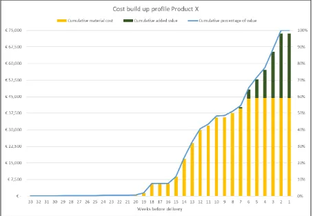
(16) 2 Research design This chapter introduces the research conducted at Company X. First, Section 2.1 describes the context of the research. Thereafter the research motivation is clarified in Section 2.2. The problem description of this research is given in Section 2.3 and the research objective is provided in Section 2.4. Then, in Section 2.5 are the research question and sub questions presented. The scope of the research is addressed in Section 2.6 and the chapter is concluded with Section 2.7, which presents the deliverables of this research.. 2.1 Research context The production and other relevant processes are shortly described in Section 1.3, and the relationship between inventory management and the production process is explained. The main topic of this research is cycle time reduction. The cycle time is defined as the Integral Cycle Time (ICT), which is the time between placement of the first purchase order for a component needed for the requested product by Company X until delivery of the order at the customer. At the moment, the ICT of Company X is relatively high and strongly dependent on lead time of components of suppliers. The ICTs vary per product between 7 and 37 weeks and is high compared to the MCTs at Company X. During the ICT, components are ordered at suppliers based on their lead times and the remaining MCT after receiving the component. This result in costs at different moments during the ICT for Company X and this can be displayed in a cost build up profile. A cost build up profile of a product shows the cumulative cost of the product during the ICT. The cumulative cost of the product depends on the cumulative material costs and the cumulative assembly costs, which is called added value. Figure 2.1 shows the cost build up profile of Product X.. Figure 2.1 - Cost build up profile Product X. 2.

(17) Logically, there are zero cumulative costs in the beginning of the ICT and if the customer receives the product, then all costs are made for the product. The cost build up profiles of the products of Company X have a relatively big tail at the left side, as can be seen in the example of Product X. This shows that there is just a small percentage of the product’s value added during a large part of the ICT. Figure 2.1 shows that only a small percentage of the total costs are made in the first 13 weeks of the ICT. Next to this, the figure shows that the assembly of Product X is executed in the last seven weeks, which is displayed by the green bars in the figure. Lastly, the figure shows that the part of the value that is added by purchasing components is bigger than the value added by assembling the product. In the context of this research, it is interesting for Company X if the ICT can be reduced by reducing or eliminating the left tail of the cost build up profiles by applying inventory management. The size of the left tail of the cost build up profile depends on the components for which costs arise in the beginning of the ICT. Therefore, high lead time components are often the cause of a big tail at the left side. The costs for these components are made in an early stage, but there is waiting time in the process of Company X due to the high lead time. This waiting time can be prevented by applying safety stocks or specific order policies for these components. The safety stock and order policies of Company X influence when the components are available in the warehouse. For this reason, safety stocks and order policies can prevent the left tail of the cost build up profile causing a high ICT. As mentioned above, the safety stocks and order policies determine the availability of components. Components are available at Company X, when these are on hand in the warehouse at the plant. If components are not on hand in the warehouse, then production cannot be done and will be delayed, which disturbs the production process and planning. As a result, the OLT and service level of the products are negatively influenced. The availability of components is not only dependent on the safety stocks and ordering policies, but also dependent on the lead time and reliability of the suppliers. This research will focus on the effects of the safety stocks and ordering policies on the ICT and OLT of Company X. The ICT and OLT are both dependent on the MCT and the availability of the needed components. If the components are not available and not ordered at the supplier, then the OLT to the customer will be at least the sum of the lead time of the supplier and the MCT. As mentioned above, the availability of components is dependent on the stock positions and ordering policies and the reliability of the supplier. The stock positions and ordering policies determine when orders are placed and which quantities are ordered. An MOQ given by the supplier for this component can affect the order quantity for this component. Next to these ordering policies, there can be a policy for a component to have a safety stock in the warehouse at the site. This safety stock can increase the availability of a component by covering uncertainty in demand of the component. The decisions made with respect to inventory management are based on the financial risks. The financial risks depend mainly on the price of the components and the holding costs. The lead time of the components of suppliers are dependent on the supplier and negotiated by the purchasing department. The involved risk shows that there is a trade-off between costs and performance. This research has to give insights in the relationship between safety stocks, ordering policies, cycle times and lead times of the products and the resulting costs and financial risks.. 3.

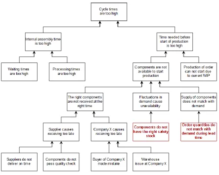
(18) 2.2 Research motivation The relatively high ICT is a motivation to execute a research into cycle time reduction by inventory management. Besides, one of the important customers of Company X requested for smaller ICTs of the products of Company X. This important customer will be called Customer Y due to confidentiality. The ICTs for a lot of products as requested by Customer Y are lower than the sum of the supplier lead time and the MCTs of Company X. This means that the ICT will be higher than requested by the customer in case the components are not on stock or not ordered at the supplier. This request of Customer Y shows the urgency of a research into reducing cycle times by inventory management. Besides, if this research shows that ICT reduction for this Customer Y is possible, then the approach can be used to reduce the cycle times of products of other customers. Next to this specific request of Customer Y, cycle time reduction is also one of the goals of supply chain management at Company X. Cycle time reduction makes it possible to respond faster to the demand of the customer. This increases flexibility of the process of the company and this flexibility makes it possible to respond to fluctuations in demand. Besides, lower cycle times can increase competitiveness and it can influence the customer satisfaction. Another aspect of reducing cycle times are the financial benefits for the company. One of the benefits is that the cash flow will change in a positive way, because the time between making costs for an order and receiving payment is shorter. Next to this, reducing the cycle times will decrease the value of open sales orders of Customer Y to Company X, because the total amount of products with open sales orders will decrease if the cycle times are reduced.. 2.3 Problem description After describing the context and motivation of this research, we need to get a clear view of the problem of this research. The problem of Company X is that the ICTs are too high. This topic is important and needs attention, because of the recent request for shorter ICTs by Customer Y. The decision is made that the norm of the ICTs will be a variable during this research and can differ per product. Currently, the ICTs of the products for Customer Y are between 7 and 37 weeks. The action problem of Company X is the difference between the actual ICT and the preferred ICT, which is dependent on the costs and risks to reduce the ICT. The next step after identifying the action problem is finding the causes of this action problem and defining the knowledge problem behind the causes. The high ICTs can have two different causes, namely that the internal assembly time is too high or that the time needed before start of production is too high. The internal assembly time is too high because of high waiting times or high processing times during the assembly process. In addition, too high lead times can be caused by too much time needed before start of production. This can be a result of the current amount of Work In Progress in production, which cannot always be prevented. Next to this, if components are not available in the warehouse, then production cannot start and waiting time is created. Unavailability of components can be a result of components that are not delivered at the right time. This is caused by the supplier or by Company X. The supplier’s side has two main causes, namely that the supplier do not deliver the components on time or the components of the supplier do not pass the quality check. The causes of Company X’s side can be a buyer mistake or issues in the warehouse, which results in not receiving the components on time. Another cause of unavailability of components in the warehouse is fluctuations in demand of components. This can be prevented by having safety stock and if components are not available due to fluctuations in demand, then the 4.

(19) components do not have the right safety stock. Lastly, if the supply of components does not match with the demand of the components, then the components are also not available to start production. This shows that order quantities do not match with the demand during lead time. The problems of not having the right safety stock and order quantities not matching with demand during lead time have a big influence on the process and performances at Company X. Company X does not have the optimal safety stock and order quantities of components to shorten their ICTs and OLTs. Currently, the safety stocks and order quantities are static and not dependent on demand of products. These causes are selected as knowledge problem for this research. The relationships between causes and identification of the knowledge problem are displayed in Figure 2.2.. Figure 2.2 - Problem cluster. 2.4 Research objective The objective of this research is identifying the relationship between an inventory management policy and the cycle times at Company X. This inventory management policy includes the sizes of the safety stocks and order quantities of components. This relationship gives insights in how the cycle times of Company X can be reduced while minimizing the financial risks and maintain the reliability to the customer. This insight should be gained by modelling the relationships between safety stocks, order policies and cycle times. After discovering, analyzing and modelling this relationship, the goal is to determine the safety stocks and order quantities of the involved components. A safety stock and specific order policy could reduce the tails of the cost build up profile of the products of Company X. If it is 5.

(20) recommended to have a safety stock, then the size of the safety stock needs to be determined. Lastly, the expected costs and risks of the policies should be estimated. The expected costs has to take the costs of inventory into account. The risks of the policies has to show the costs of ordering components without having a SO of the customer at that time. Then Company X can negotiate with Customer Y about liabilities for these costs.. 2.5 Research questions The problem as described in the previous sections lead to the following research question:. Which inventory policy should be used at Company X to reduce the Integral Cycle Times of the products for Customer Y taking into account financial risks and reliability risks? The answer to this research question is obtained with several sub questions. Based on the research problem and the steps of a general managerial problem-solving method (Heerkens & Van Winden, 2012), four sub questions are formulated. These sub questions and a brief description of the content are discussed below: 1) What is the current situation at Company X with respect to inventory policy and resulting cycle times? a) What does the inventory management process at Company X look like? b) What are values and correlations of the current cycle and lead times? c) What are the causes of the cycle times higher than the norm cycle time? d) Which causes should be taken care of to improve the cycle times of Company X? 2) What methods are suggested in the literature to achieve smaller cycle times considering the inventory policy? a) Which methods are suggested in the literature to reduce the cycle times with the use of a proper inventory policy? b) What are the preconditions, assumptions and restrictions of those methods? c) What are the preferences, restrictions and limitations from the company? d) Which methods can be used to reduce the cycle times at Company X given the preconditions, assumptions and restrictions? 3) What are the performances of the alternatives regarding the cycle times and the other KPIs of Company X in a model/simulation? a) How should the performances of the cycle times and other KPIs be measured and assessed? b) What is the scope of the model and which assumptions are made to construct the model? c) What data is required to construct, validate and execute the model? d) What is the output of the model and how should it be interpreted? 4) How should the inventory policy be implemented and monitored at Company X? After answering these sub questions, the research question is answered and the conclusion to the research problem is drawn.. 6.

(21) 2.6 Scope This research will focus on reducing the cycle times with safety stocks and ordering policies. The production process (i.e. MCT) is not extensively analyzed during this research, because the needed cycle time reduction cannot be achieved by reducing the cycle times in production. Because of the request for smaller cycle times from Customer Y, the products and items related Customer Y are taken into account in this research. Customer Y orders around 150 different products, with different components in their Bill Of Material (BOM). In the current situation analysis are all products and underlying components into account. Later in this research, the decision is made that the scope of products in the model is reduced to 86 products. Those products are volume products with reliable data. The other products are NPIs or EOL products, which means that the underlying components can have a different inventory policy. Focusing on these products of Customer Y keeps the project manageable within the given time window. Despite, some of the results and insights of this research and eventually the model can be partly applied to more customers within Company X.. 2.7 Deliverables This research consists of a number of deliverables: -. -. A qualitative and quantitative analysis of the current lead times, safety stocks and ordering policies. A model that gives insights in the risks with respect to costs, liabilities and reliability. There is a manual or tool delivered next to this model to make it usable for Company X in the future. (Specifying what can be expected and what is feasible) An advice how the model and generated output should be implemented at Company X.. 7.

(22) 3 Current situation analysis This chapter describes an analysis on the current situation at Company X. Executing qualitative interviews with the stakeholders of the problem is the first step of the analysis. In Section 3.1 are the outcomes of those interviews described and discussed which variables are important during this research. In the following sections are the relevant variables described and quantified. The information described in those section are used to discuss the high ICT and its causes in Section 3.8. The chapter ends with Section 3.9, which gives a conclusion of this chapter and answers the first research question mentioned in Section 2.5: What is the current situation at Company X with respect to inventory policy and resulting cycle times?. 3.1 Qualitative analysis To analyze the current situation regarding inventory management and the performances of Company X, we need to describe the process and related parameters and variables. In Section 1.3 is the process at Company X already shortly described, but in this Section we will go into more detail. The connection with the related information systems gets attention, because relevant data for this research is stored and monitored in those systems. As mentioned earlier, production requires having the right components in the warehouse at the right time. Managing this process is called inventory management, which has the objective to minimize inventory investment subject to achieving a minimum level of customer service (Hopp & Spearman, 2008). In the case of Company X, customer service is partly expressed in ICT in weeks and percentage of on time deliveries. Both components of customer service are related to each other, because shortening the ICTs could result in a lower percentage of on time deliveries. At Company X are different variables involved in the inventory management process. The values of the involved variables are determined and this is stored in Rapid Response. Rapid Response is one of the IT systems of Company X to store data of their products and processes. The following variables are related to the ICT and inventory management process: -. Lead time of components Internal assembly time of subassemblies and products Safety stock of components Minimum Order Quantity (MOQ) of components. The first mentioned variable is the lead time of the component. This can be divided in fixed lead time and safety lead time. The fixed lead time of a component is negotiated with the supplier. Despite, the safety lead time is determined by Company X based on uncertainties in the processes related to the involved component. Those safety lead times are static, which could make them less accurate. Next to the lead time of the suppliers, the internal assembly times influence the lead time and determine when components need to be in the warehouse. A third important variable is the safety quantity of a component, which can also be called safety stock or safety inventory. This is the amount of inventory of a component held in case demand exceeds expectations; it is held to counter uncertainty (Chopra & Meindl, 2013). Next to this, components can have a MOQ, which can influence the inventory management process. Lastly, there are Key Performance Indicators (KPIs) involved with inventory management and this research. In the case of Company X, the amount of inventory on hand. 8.

(23) and inventory turnover are important indicators of the performances with respect to inventory management.. 3.2 Lead times of components The current situation analysis will focus on the 154 products sold to this specific customer, who requested shorter cycle times. Production of these products require purchasing 4,367 components from 127 different suppliers. The lead times of these components stored in the ERP-system vary in a range of 1 week until 46 weeks. Figure 3.1 shows a histogram of the lead times of components. The control of the inventory of components with a long lead time is most critical, because those components can have big influence on the cycle times and on time deliveries. As can be seen in Figure 3.1, the percentage of components with a lead time above 63 days (9 weeks) is more than 25% and even more than 10% of the components have a lead time of 182 days (26 weeks) or longer. A large part of those last ten percent of components is allocation parts. The lead times of allocation parts is uncertain and dependent on the current market situation. In general, Company X assumes a lead time of 26 weeks for those components. This seems to be a good assumption based on recent deliveries of those parts. Therefore, the lead time of allocation parts involved in this research is determined as 26 weeks.. Figure 3.1 - Histogram of lead time of components (March 1, 2019). The above described lead times are committed with the suppliers. Unfortunately, the suppliers do not always deliver within the lead time. The supplier can cause delivering not on time, but also Company X delays deliveries on purpose. A reason for that can be delaying the start date of production. In that case, if the suppliers do not deliver on time, then it does not have a direct impact on the production. In Figure 3.2, the blue bars show the percentages of purchase orders, which are not delivered on time. And the green bars show the percentage of not delivered purchase orders with production impact. In other words, the green bars show which part of the blue bars have production impact. Those percentages are calculated based on planned purchase order deliveries per week. The percentage of purchase orders not 9.

(24) delivered is relatively high and week 5 of 2019 shows an extreme value. Despite, the percentages of not delivered purchase orders with production impact is lower. This value varies around 10 percent in the last nine weeks, which means that between 50 and 150 purchase orders are not delivered and result in impact on production. This confirms the need for a proper inventory policy to respond to these uncertainties at the supplier side of the supply chain. Therefore, these uncertainties need to be modelled in the right way to determine a proper inventory policy. The decision is made to focus in this research on reducing the lead times by anticipating on uncertainties instead of improving the supplier performances.. Figure 3.2 - Delivery reliability of purchase orders. 3.3 Internal assembly times The second important variable related to the cycle time is the internal assembly time of a product. The internal assembly time of a product consist of assembling all components and/or subassemblies to get the product. Subassemblies are a result of assembling components in a production step and these subassemblies are used in a sequencing production step, which will result in another subassembly or end product. Those internal assembly times do include processing time, but also waiting times in production. Company X has determined the internal assembly time based on experience with the particular product. There is made a distinction between products produced in the PCBA department and the Clean Room/White Room (CR WR) department. A histogram of the internal assembly times of the products delivered to Customer Y are displayed in Figure 3.3. The figure shows that all products have assembly times smaller or equal to twenty working days, which is exactly four weeks. Besides most of the products have an internal assembly time of one, two or three weeks. The figure shows that the PCBA products do have more frequent an internal assembly time of 15 working days compared to the CR WR products. Therefore, it can be useful in the modelling phase to distinguish PCBA products from CR WR products, because of different internal assembly times.. 10.

(25) Figure 3.3 - Internal assembly times (March 1, 2019). The length of the internal assembly time of products determines in which stage of the cycle time components and subassemblies need to be on hand. Products with higher assembly times need to have the components or subassemblies available in an earlier stage of the cycle time. Important note is that subassemblies need to be produced before the product can be assembled. The subassemblies are divided in to two groups, PCBA subassemblies and CR WR subassemblies. Figure 3.4 shows a histogram of the lead times of PCBA subassemblies, CR WR subassemblies and both types together. In general, the assembly times of PCBA subassemblies are higher than the assembly times of CR WR products. This is caused by the wire harnesses, which are grouped in the CR WR subassemblies. The wire harnesses have short internal assembly times and cause the higher frequency at five days.. Figure 3.4 - Internal assembly times subassemblies (March 1, 2019). 11.

(26) The internal assembly times of subassemblies increases the total internal assembly time of a product. As mentioned above, there is a specific sequence of assembling different subassemblies and end products. Therefore, this precedence constraint has to be modelled to determine the right inventory policy of the components needed for the products. The sum of the internal assembly time of the subassemblies and the internal assembly time of the product indicates when a component needs to be available at Company X. The precedence constraint can be displayed in a precedence diagram. Figure 3.6 shows a precedence diagram of a product for Customer Y, where every node is a production step in the process where is subassembly is assembled. The diagram shows the sequence of the assembly process of 27 different subassemblies into the end product. The subassemblies are numbered from 1 to 17 and if the nodes are serial, then there is a precedence constraint between subassemblies. Next to this, the diagram shows that the last assembly step consist of assembling seven subassemblies and components into the product. The longest path in the precedence diagram results in the minimum internal throughput time of the product, because this amount of time is needed to execute that sequence of assembly steps. As mentioned above, the precedence relationships and internal assembly times result in a minimum internal throughput time, which Company X calls lead time makes only. For every end product are these relationships and corresponding internal assembly times known. Given these knowledge and values, the lead time makes only can be determined for every product. Figure 3.5 displays a histogram of the lead time makes only of products. The histogram shows that there are several products with a lead time longer than 45 working days (9 weeks). Despite, Company X calculates one week safety time within this lead time which increases the lead time of every product with 5 working days. The products with a longer lead time makes only are mainly products with subassemblies from the PCBA department. This lead time makes only will be used to determine when components need to be on hand, but this research will not investigate opportunities to reduce those lead time makes only.. Figure 3.5 - Histogram of lead time makes only of end products (March 20, 2019). 12.

(27) Figure 3.6 - Precedence diagram of production steps to produce Product X. 3.4 Safety stock for components The third important variable related to the inventory policy is the safety stock at Company X. Company X uses safety stock to mitigate the risk of a shortage of material and absorb the variability in customer demand. Important is to determine where and at which level the safety stock is held. The level and place of the safety stock determines the flexibility and costs. For Company X, this results in several options with respect to using safety stock. By negotiating and taking it down level for level results in finding the right level of safety stock. Figure 3.7 shows how Company X should execute this procedure of finding the right level for safety 13.

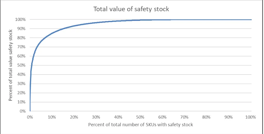
(28) stock. For Company X resulted this procedure in applying safety stocks for components without safety stocks for products or subassemblies. Despite this theoretical approach for selecting at which level safety stock are applied, the determination of the amount of safety stock is not based on theory or calculations at Company X. Currently, components have safety stock if there were issues in the past with that component and the size is determined based on expertise knowledge.. Figure 3.7 - Company X's safety stock options. After deciding at which level safety stocks are used, the sizes of the safety stocks have to be determined. As mentioned earlier, for the production of the products of Customer Y are 4,367 components purchased. Company X decided to use safety stocks for 1,104 components. All the other components do not have a safety stock regarding the data of Rapid Response. Table 3.1 gives an overview of the numbers presented above. Table 3.1 - General safety stock statistics (March 1, 2019). General safety stocks statistics Number of end products Number of end products with safety stock Number of subassemblies Number of subassemblies with safety stock Number of components Number of components with safety stock Number of components without safety stock. 154 0 305 0 4,367 1,104 3,263. The amount of safety stocks are often dependent on characteristics of the components. The lead time, variations in those lead time and demand of a component are the most important characteristics to determine safety stocks of a components for a company. Despite, the value of a component is an important characteristic for a company to decide about the safety stock sizes. Comparing safety stocks of different components and analyzing the current safety stock sizes is complex due to the dependency on the various characteristics of the components. Besides many components of Company X are used in different subassemblies and/or products. This means that different internal assembly times are involved in the calculations of the right safety stock. The current safety stocks of Company X are static and there is no clear reasoning behind the sizes of the current safety stocks. There is also a lack of reasoning 14.

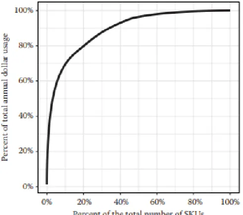
(29) behind having no safety stocks for components. The sizes of safety stock vary between 1 and 20,435 for a single component. The total size of safety stock of all 1,104 components is 600,541. Even more important is the cost related to the safety stock. Therefore, the total values of the safety stock of a component, which will be called later on Stock Keeping Unit (SKU), gives insight in the proportional costs between different components. The total values per SKU do also vary within a wide range, namely € 0.01 and € 35,000. Company X has with their current safety stock sizes a total value of € 316,326.41 in their warehouse. The total value of safety stock per SKU is calculated by multiplying the standard cost and the safety stock size of the SKU. The total value of safety stock per SKU can also be expressed in a percentage of the total value of the safety stocks of all SKUs. Ranking the SKUs based on total value in descending order and calculating the cumulative percentage of the total value of the safety stocks of all SKUs results in Figure 3.8. The graph shows that a small number of the components contribute to a big percentage of the total value of the safety stock, which indicates that the Pareto principle is applicable to the total value of safety stocks. This is quantified with the fact that 10 percent of the SKUs with safety stock contribute to 85% to the total value of the safety stock. Besides, the figure shows that the last 50% of the number of SKUs contribute to less than 1% to the total value of the safety stocks. These numerical facts show the differences in total value in the safety stocks per SKU.. Figure 3.8 - Relation between total value of safety stock and number of SKUs (March 1, 2019). This research have to give insight in the optimal safety stocks needed to achieve the shorter ICTs with minimized costs. Therefore, it is important to analyze the components without safety stock and find out whether it is necessary to use safety stock for those components to reduce the ICT. There are 3,263 components at Company X without a safety stock. This does not have to be a problem if components have short lead times or if there are not a lot of uncertainties in supply or demand. The inventory management of components with a long lead time is important, otherwise the ICT will not be reduced.. 15.

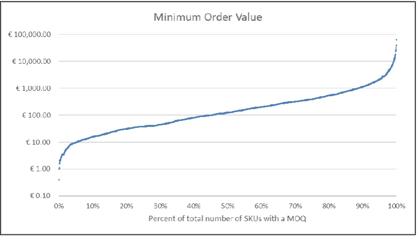
(30) 3.5 Minimum Order Quantity for components Another relevant variable of the components involved in this research is Minimum Order Quantity (MOQ). MOQ is defined as the required minimum quantity of a component per order. Those minimums are typically a result of supplier requirements, for example raw material availability, factory set-up or packaging type. Therefore it is not possible to adjust MOQs of components instead of this Company X has to deal with the MOQs while managing their inventory. The MOQ does not give information about financial risks, because a high MOQ of a component with a low standard cost does not result in high financial risks. Therefore, a minimum order value is calculated, which is equal to the multiplication of the MOQ and the standard cost of the SKU. This minimum order value can indicate financial risks resulting from the MOQ. Figure 3.9 displays the minimum order value of SKUs with a MOQ. There is a logarithmic scale used in the graph to make the difference in value easier to read. The figure shows that around 90% of the components with a MOQ have a minimum order value of less than € 1,000. Besides, around 1% of the components have a minimum order value of more than € 10,000. Most of those components have a high standard cost per component instead of a high MOQ. The biggest outlier of the minimum order value is caused by a high MOQ, which resulted in a minimum order value of € 63,828.. Figure 3.9 - Minimum Order Values of SKUs with a MOQ (March 1, 2019). The financial risks also depend on the demand and lead time of the component. Those factors determine how long it takes before Company X uses the components in production and deliver them to the customer. After delivery, Company X receive the payment from the customer and the financial risks are zero for the components. Therefore, higher demand or shorter lead times result in smaller financial risks. Logically, if the demand during lead time is bigger than the MOQ, there are no extra financial risks caused by the MOQ.. 3.6 Inventory On Hand The first KPI of inventory management is the amount of inventory on hand expressed in value, which takes into account components, subassemblies and end products. The inventory on hand is an indicator for the financial risk related to the inventory management process. This financial risk is created by a time gap between paying the supplier for the component and 16.

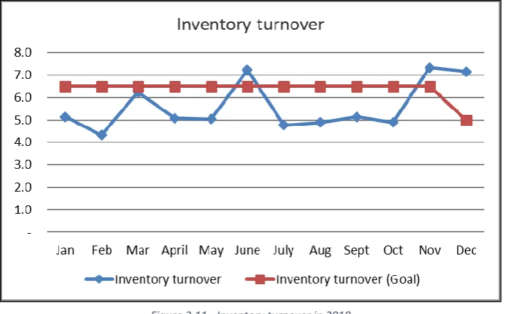
(31) receiving the payment of the customer for the product. In this research, the amount of inventory hold for Customer Y is only taken into account. Therefore, for every month in 2018 is the amount of inventory on hand for Customer Y determined. This value is dependent on the sales and operations planning of Company X, because increasing sales will result in a higher amount of inventory on hand. The inventory on hand has to be compared with the projected amount of inventory and the corporate goal of the amount of inventory. Figure 3.10 shows the development of the amount of inventory on hand per month through 2018. The graph shows that the inventory on hand decreased in the second part of the year. Next to this, the inventory on hand comes closer to or becomes even less than the inventory on hand projection in the last months of 2018. In general, companies always have the goal to reduce the amount of inventory on hand. Despite, this research focusses on reducing the cycle time for products for Customer Y. Therefore, an analysis of the amount of inventory on hand always have to take the performances of the company with respect to cycle time or sales into account.. Figure 3.10 - Inventory On Hand in 2018. 3.7 Inventory turnover The second KPI related to inventory management at Company X is the inventory turnover of the total inventory on hand, which includes components, subassemblies and end products. The inventory turnover measures the number of times inventory turns over in a year. (Chopra & Meindl, 2013) It is the ratio of average inventory to either the cost of goods sold or sales. The cost of goods sold is relevant in this research, because the management of inventory of components is investigated. The following formula is used to calculate the inventory turns: 𝐼𝑛𝑣𝑒𝑛𝑡𝑜𝑟𝑦 𝑡𝑢𝑟𝑛𝑜𝑣𝑒𝑟 =. 𝐶𝑜𝑠𝑡 𝑜𝑓 𝑔𝑜𝑜𝑑𝑠 𝑠𝑜𝑙𝑑 𝑖𝑛 𝑚𝑜𝑛𝑡ℎ∗12 𝐴𝑣𝑒𝑟𝑎𝑔𝑒 𝑖𝑛𝑣𝑒𝑛𝑡𝑜𝑟𝑦 €. ( 3.1 ). Inventory turnover can be a very useful measure, especially when comparing divisions of a firm or firms in an industry. (Silver, Pyke, & Thomas, 2017) Firms in different industries or with a different strategy can have different inventory turnovers due to a difference in for example Work In Progress. Therefore, strategic competitive advantage can have a significant effect on the determination of the appropriate inventory turnover number. (Silver, Pyke, & Thomas, 2017) The equation of the inventory turnover shows that an increase in sales without a 17.

(32) corresponding increase in inventory will increase the inventory turnover, as well a decrease in inventory without a decline in sales. During this research, the goal is to reduce the cycle time by applying efficient inventory management. Therefore, the objective is to have an appropriate inventory turnover instead of maximizing the inventory turnover, because otherwise the requested cycle time will not be achieved. The inventory turnover per month of Company X in 2018 is shown in Figure 3.11. The number have to be compared with the corporate goal, which is for the first eleven months 6.5. The figure shows that in most months the inventory turnover is lower than the goal of 6.5. There are three exceptions and two of them are in the last months of the year. The higher inventory turnover are mainly caused by a decrease in inventory on hand.. Figure 3.11 - Inventory turnover in 2018. 3.8 Causes of high lead times The previous sections describes the aspects and variables related to the cycle time of the products for Customer Y at Company X. This cycle time influence directly the committed lead time for the products with Customer Y. The Order Lead Time (OLT) is defined as the total time between confirming SO and delivering the order at the customer. A part of this lead time is used for assembling components to subassemblies and sequentially assembling the end products. In the past, Company X and Customer Y agreed about OLTs for the products and applied those lead times in their supply chain. Figure 3.12 shows the percentage of products with a specific lead time between 0 en 40 weeks. This confirms that not only the ICTs of Company X are high, but also the OLTs are high. The above described analysis of the different aspects of the cycle time and lead time already showed which causes should be investigated in this research. Mainly the long lead times of components and relatively short internal assembly times of subassemblies and products showed the urgency of improving the inventory management of components. The lead times of components showed that reducing the cycle time and lead time is not achievable without having safety stocks or open orders at suppliers. Besides, the percentage of late deliveries of suppliers with impact on production confirmed that executing a research into the safety stocks is necessary. This can be beneficial for the cycle and lead time, but also reduce the disruptions in the planning and production departments. 18.

(33) Figure 3.12 - Histogram of lead times products. 3.9 Conclusion This chapter describes an analysis of the current situation of inventory management at Company X. This analysis results in an answer to the first research question: What is the current situation at Company X with respect to inventory policy and resulting cycle times? First, it is important to understand which aspects determine the cycle times. Therefore, Section 3.1 describes which variables are relevant during this research. As mentioned earlier, the first part of the process consists of purchasing components at suppliers. Therefore, the current situation with respect to lead times of components and the reliability of those lead times are important for the inventory policy and resulting cycle times of products. Section 3.2 elaborates on the lead times of components and shows that those lead times are relatively long compared to the cycle time and lead time of products. Besides, this section shows that the supplier do not always deliver the components within the agreed lead time, which results in disruptions in the production and planning processes. The production processes consist of assembling subassemblies and sequentially assembling the product. Section 3.3 quantifies the internal assembly times of products and subassemblies. Those assembly times are relatively short compared to the lead time of components. Those first two sections confirm that the cycle times have to be reduced by applying the right inventory policies for components. In Section 3.4 is described what the current situation is with respect to safety stocks. At Company X, safety stocks are only applied at component level. However, a large part of components does not have a safety stock. Besides, there is no clear explanation for the current safety stock and they are often not aligned with the demand and order quantities of the components. The order quantities have to be determined during this research given the MOQs of components, which are shortly discussed in Section 3.5. In the case of the components relevant for this research, most of the MOQs do not result in extreme order values. 19.

(34) Another important aspect of inventory management is the financial side of having inventory. Section 3.6 discusses the historical amount of inventory on hand for Customer Y and compares this with the projection and goal. The research has to take the amount of inventory into account when optimizing the inventory management. And Section 3.7 shows that the inventory turnover of Company X is in general lower than the corporate goal, which also confirms the need for an improved inventory policy. Section 3.7 relates the different aspects of cycle and lead time with the current lead times. This section shows that the inventory management of Company X should be investigated. In the upcoming chapter, there is literature related to inventory management presented. The literature study focusses on inventory policies, item classification, calculating safety stock and reorder points, because this chapter confirmed that with the current management of inventory is it not possible to reduce the cycle time and lead time. The analysis of this literature has to give insights in how inventory management can be applied to reduce cycle times and lead times at Company X. Thereafter, there is a model constructed to determine which inventory policy should be applied. This model has to take financial risk into account. Besides, the input of the model has to be configurable and generic to make it possible to implement it at Company X over a longer time horizon.. 20.

(35) 4 Literature review Now the problem and current situation of Company X are clear, this chapter will present relevant inventory management concepts and link them to the situation within Company X. The inventory management concepts are retrieved from existing literature. The importance of inventory management and the relevant types of inventory are described in Section 4.1. Thereafter, Section 4.2 elaborates on different inventory control policies and their advantages and disadvantages. Thereafter, Section 4.3 gives insights in classification methods, which can be applied to select different inventory policy per class. In the following three sections is theory about the Economic Order Quantity (EOQ), reorder point and safety stock presented. These sections will also present the corresponding formulas. In Section 4.7 is presented how the literature can be applied in the research’s context. This chapter will be closed by a conclusion in Section 4.8 with an answer to the following research question: What methods are suggested in the literature to achieve smaller cycle times considering the inventory policy?. 4.1 Inventory management The strategic benefits of inventory management have become obvious since the mid-1980s. Nowadays many firms coordinate with other firms in their supply chains. Instead of responding to unknown and highly variable demand, companies in the supply chain share information so that the variability of the demand they observe is significantly lower (Silver, Pyke, & Thomas, 2017). The objective of a company is having an effective and efficient inventory control. Companies try to reduce inventories to decrease the costs of inventory. Nevertheless, there are limits on reducing inventories, because companies cannot perform at a competitive level without inventories. The most important and relevant reasons for having inventories are: -. Economies of scale Shortening cycle times to the customers Buffering against uncertainties in supply and/or demand. 4.1.1 Functional classification of inventories The term inventory does not clearly specify the function of the involved inventory. For this reason, Silver, Pyke, and Thomas (2017) provide functional classifications of inventories. The following classification of inventory types is made: -. -. Cycle inventories:. inventories resulting from ordering or producing batches. Congestion stocks: inventories due to items competing for limited capacity. Safety stocks: inventories to anticipate on uncertainty of demand and the uncertainty of supply. Anticipation inventories: stock accumulated in advance of an expected peak in sales. Pipeline inventories: goods in transit between levels of a multi-echelon distribution system or between adjacent workstations in a factory. Decoupling stocks: inventories used in a multi-echelon situation to permit the separation of decision making at the different echelons. 21.

(36) 4.1.2 Cycle and safety inventory In this research, the cycle inventories and safety stocks are investigated and the other types of inventory are not relevant for the situation of Company X. As mentioned above, cycle inventory is caused by ordering or producing batches. Chopra and Meindl (2013) do have a similar definition as Silver, Pyke and Thomas (2017), namely cycle inventory is the average inventory in a supply chain due to either production or purchases in lot sizes that are larger than those demanded by the customer. The reasons for larger lot sizes include economies of scale, quantity discounts in purchase price or freight cost, and technological restrictions. This results in a trade-off between ordering and freight costs and inventory costs for a company. The frequency of orders directly influences the amount of cycle stock on hand at any time. Less frequently ordering results in larger order sizes, which results in a higher cycle inventory. Figure 4.1 shows the relationship between order size (Q) and cycle inventory given deterministic and constant demand. Safety stock is the amount of inventory kept on hand to allow for the uncertainty of demand and the uncertainty of supply in the short run (Silver, Pyke, & Thomas, 2017). Therefore, safety stocks are not needed when the future demand and the length of time it takes to get complete delivery of an order are known with certainty. The level of safety stock is directly related to the desired level of customer service. This results in a tradeoff between holding costs and customer service level. Desiring a higher level of customer service results in a higher level of safety stock, which increases the holding costs. The influence of safety stock on the inventory profile is displayed in Figure 4.1. Higher safety stock results in higher inventory levels and a higher average inventory, which means that the financial investment will be higher. Important to note is that Figure 4.1 shows an inventory profile with a deterministic and constant demand. However, in this research annual demand will be modelled as deterministic demand, but there are fluctuations in the weekly demand. Despite, the definition of cycle and safety inventory is the same in both cases.. Figure 4.1 - Inventory profile with cycle and safety inventory (Kim). 22.

No results found