Artificial bee colony algorithm with time varying strategy

(1)

Research Article

Artificial Bee Colony Algorithm with Time-Varying Strategy

Quande Qin,

1,2

Shi Cheng,

3,4

Qingyu Zhang,

1,2

Li Li,

1

and Yuhui Shi

5

1_{Department of Management Science, College of Management, Shenzhen University, Shenzhen 518060, China} 2_{Research Institute of Business Analytics & Supply Chain Management, Shenzhen University, Shenzhen 518060, China} 3_{Division of Computer Science, University of Nottingham Ningbo China, Ningbo 315100, China}

4_{International Doctoral Innovation Centre, University of Nottingham Ningbo China, Ningbo 315100, China} 5_{Department of Electrical & Electronic Engineering, Xi’an Jiaotong-Liverpool University, Suzhou 215123, China}

Correspondence should be addressed to Shi Cheng; [email protected]

Received 29 October 2014; Revised 13 March 2015; Accepted 17 March 2015

Academic Editor: Ricardo L´opez-Ruiz

Copyright © 2015 Quande Qin et al. This is an open access article distributed under the Creative Commons Attribution License, which permits unrestricted use, distribution, and reproduction in any medium, provided the original work is properly cited.

Artificial bee colony (ABC) is one of the newest additions to the class of swarm intelligence. ABC algorithm has been shown to be competitive with some other population-based algorithms. However, there is still an insufficiency that ABC is good at exploration but poor at exploitation. To make a proper balance between these two conflictive factors, this paper proposed a novel ABC variant with a time-varying strategy where the ratio between the number of employed bees and the number of onlooker bees varies with time. The linear and nonlinear time-varying strategies can be incorporated into the basic ABC algorithm, yielding ABC-LTVS and ABC-NTVS algorithms, respectively. The effects of the added parameters in the two new ABC algorithms are also studied through solving some representative benchmark functions. The proposed ABC algorithm is a simple and easy modification to the structure of the basic ABC algorithm. Moreover, the proposed approach is general and can be incorporated in other ABC variants. A set of 21 benchmark functions in 30 and 50 dimensions are utilized in the experimental studies. The experimental results show the effectiveness of the proposed time-varying strategy.

1. Introduction

Swarm intelligence concerns the design of intelligent opti-mization algorithms by taking inspirations from the collec-tive behavior of social insects [1]. During the past decades, swarm intelligence has shown great success for solving complicated problems. The problems to be optimized by swarm intelligence algorithms do not need to be mathemati-cally represented as continuous, convex, and/or differentiable functions; they can be represented in any form [2]. Artificial bee colony (ABC) algorithm developed by Karaboga in 2005 is a recent addition into this category [3–5].

ABC algorithm is inspired by the intelligent behavior of honey bees seeking quality food sources [3, 6–8]. In a short span of less than 10 years, ABC has already been demonstrated as a promising technique for solving global optimization problems [9, 10]. Numerical comparisons and

many engineering applications demonstrated that ABC could obtain good search results [11]. Due to its simplicity, flexibility, and outstanding performance, ABC has captured increasing interests of the swarm intelligence research community and been applied to many real-world areas, such as numerical optimization [6,10], neural network training [7,12], finance forecasting [13,14], production scheduling [15–17], data clus-tering [18,19], image segmentation [20,21], service selection problem [22], and power system optimization [23].

However, like its counterpart population-based stochastic algorithms, it still has some inherent pitfalls [24–26]. The convergence speed of ABC is slower than those of the representative population-based stochastic algorithms, such as DE and PSO [27]. Moreover, ABC suffers from premature convergence while dealing with certain complicated prob-lems [28]. Several ABC variants have been proposed with the aim of overcoming these pitfalls. These ABC variants

(2)

can be generally categorized into three groups: (1) first, the parameters of configuration tuning [29–31]; (2) second, the ABC algorithm hybridizing with other evolutionary optimization operators to enhance performance [10,32,33]; (3) third, the design of new learning strategy by mod-ifying the search equation of the basic ABC algorithm [24,25,34].

It is recognized that exploration and exploitation are the two most important factors affecting a population-based optimization algorithm’s performance [6, 35]. Exploration refers to the ability of a search algorithm to investigate the unknown regions in the search space in order to have high probability to discover good promising solutions. Exploitation, on the other hand, refers to the ability to concentrate the search around a promising region in order to refine a candidate solution [36, 37]. A good population-based optimization algorithm should properly balance these two conflictive objectives [38]. It is observed that ABC has good exploration ability but poor exploitation ability [24], which may impede ABC algorithm from proceeding towards a global optimum even though the population has not converged to a local optimum.

The colony of the ABC algorithm contains three groups of bees: employed bees, onlookers, and scouts [3]. In the employed bees phase of ABC algorithm, the algorithm focuses on the explorative search indicated by the solu-tion updating scheme, which uses the current solusolu-tion and a randomly chosen solution. A fitness-based probabilistic selection scheme is used in the onlooker phase, which indicates the exploitation tendency of the algorithm. In the original ABC algorithm, it is assumed that half of the colony consists of the employed bees, and the rest half consists of the onlookers [3]. In other words, the ratio of the employed and onlooker bees is the same, 1 : 1.

The basic ABC algorithm is easy to tune with few parameters but lacks effective and efficient ways to control the exploration ability and exploitation ability. In the present study, we propose an easy modification to the structure of the basic ABC algorithms in an attempt to balance their exploration and exploitation abilities. Compared with the basic ABC algorithm, we added a new parameter. The core idea of the modification is to design a proper mechanism, adjusting the ratio of the employed and onlooker bees with time. The proposed algorithms are called ABC with linear versus nonlinear time-varying strategy (ABC-LTVS and ABC-NTVS, resp.). The objective of this development is to enhance the global exploration in the early search and to encourage the solution to converge toward the global optima at the later search.

The reminder of this paper is organized as follows: Section 2briefly introduces the basic ABC algorithm. The proposed algorithms, ABC-LTVS and ABC-NTVS, are elabo-rated inSection 3. InSection 4, comprehensive experimental studies are conducted on 21 benchmark functions in 30 -dimension and50-dimension problems to verify the effec-tiveness of the proposed algorithms. Finally, conclusions are presented inSection 5.

2. Basic ABC Algorithm

The ABC algorithm is a recently introduced optimization algorithm proposed by Karaboga [3,39,40], which is inspired by the intelligent foraging behavior of the honeybee swarm. In the ABC algorithm, there are two components: the forag-ing artificial bees and the food source [3,39]. The position of a food source represents a possible solution. The nectar amount of a food source corresponds to the fitness of the associated solution. In the basic ABC algorithm, the colony of artificial bees contains three groups of bees: employed bees, onlookers, and scouts. The employed bees are responsible for searching available food sources and pass the food information to the onlooker bees [3, 40]. The onlookers select good sources from those found by the employed bees to further search the foods. When the fitness of the food sources is not improved through a predetermined number of cycles, denoted aslimit, the food source is abandoned by its employed bee, and then, the employed bee becomes a scout and starts to search for a new food source in the vicinity of the hive.

The ABC algorithm consists of four phases: initialization, employed bees, onlooker bees, and scout bees [3,39,40]. In the initialization phase of the ABC, SN food source positions are randomly produced in the𝐷-dimensional search space using the following equation [3,6]:

V_𝑖𝑑= 𝑙_𝑑+ 𝑟₁(𝑢_𝑑− 𝑙_𝑑) , (1)

where ⃗𝑥_𝑖 = [𝑥_𝑖1, 𝑥_𝑖2, . . . , 𝑥_𝑖𝐷] is the 𝑖th food source, 𝑑 ∈ {1, 2, . . . , 𝐷};𝑖 ∈ {1, 2, . . . ,SN}, where SN denotes the number of food source;𝑙_𝑑and𝑢_𝑑are the lower and upper bounds for dimension𝑑, respectively;𝑟₁is a random number uniformly distributed within range[0, 1].

After producing food sources and assigning them to the employed bees. There is only one employed bee on each food source. In the employed bee phase of ABC, each employed bee tries to find a better quality food source based on ⃗𝑥_𝑖. A new trial food source, denoted as ⃗𝑢_𝑖 = [𝑢_𝑖1, 𝑢_𝑖2, . . . , 𝑢_𝑖𝐷], is calculated from the equation below [3,6]:

𝑢_𝑖𝑗= 𝑥_𝑖𝑗+ 𝜙 (𝑥_𝑖𝑗− 𝑥_𝑘𝑗) , (2)

where𝑗is a randomly generated whole number in the range [1, 𝐷];𝜙 is a random number uniformly distributed in the range[−1, 1]; and𝑘is the index of a randomly chosen food source satisfying𝑘 ̸= 𝑖. After ⃗𝑢_𝑖is obtained, it will be evaluated and compared to ⃗𝑥_𝑖. If the fitness of ⃗𝑢_𝑖is better than that of

⃗𝑥

𝑖, the bee will forget the old food source ⃗𝑢𝑖and memorize

the new one. Otherwise, it keeps ⃗𝑥_𝑖 in her memory. After all employed bees have finished their search, they share the nectar and position information of their food sources with the onlookers.

Each onlooker bee selects a food source of an employed bee to improve it. The roulette selection mechanism is performed by using(3)[3,6]

𝑝_𝑖= fit( ⃗𝑥𝑖) ∑SN

𝑗=1fit( ⃗𝑥𝑗)

(3)

(1) Initialize the set of food sources ⃗𝑥_𝑖,𝑖 = 1, 2, . . . ,SN; (2) Evaluate each ⃗𝑥_𝑖,𝑖 = 1, 2, . . . ,SN;

(3) whilehave not found “good enough” solution or not reached the predetermined maximum number of iterationsdo

(4) for𝑖 = 1to SN do /∗Employed bees phase∗/

(5) Generate ⃗𝑢_𝑖with _𝑖⃗𝑥 using(2); (6) Evaluate ⃗𝑢_𝑖;

(7) if fit( ⃗𝑢_𝑖) ≥fit( ⃗𝑥_𝑖)then (8) ⃗𝑥_𝑖= ⃗𝑢_𝑖;

(9) for𝑖 = 1to SN do /∗Onlooker bees phase∗/

(10) Select an employed bee using(3);

(11) Try to improve food source quality according to Steps (5)–(8);

(12) Generate a new randomly food source for those does not improve with successive𝑙𝑖𝑚𝑖𝑡

iterations /∗Scout bees phase∗/;

(13) Memorize the best food source achieved so far;

Algorithm 1: The pseudocode of artificial bee colony algorithm.

where𝑝_𝑖is the probability of food source ⃗𝑥_𝑖being selected by an onlooker bee and fit( ⃗𝑥_𝑖)is the fitness of ⃗𝑥_𝑖. The fitness of the food sources are defined as [3,6]

fit( ⃗𝑥_𝑖) = { { { { {

1

1 + 𝑓 ( ⃗𝑥_𝑖), 𝑓 ( ⃗𝑥𝑖) ≥ 0, 1 + 󵄨󵄨󵄨󵄨𝑓 ( ⃗𝑥𝑖)󵄨󵄨󵄨󵄨 , 𝑓 ( ⃗𝑥𝑖) < 0,

(4)

where𝑓( ⃗𝑥_𝑖)is the objective function value of ⃗𝑥_𝑖. Once the onlooker has selected a food source, a new candidate food source can be obtained by (2). As in the employed bees, the greedy selection between these two food sources was performed.

If a food source, ⃗𝑥_𝑖, cannot be improved for a predeter-mined number of cycles, referred to aslimit, this food source is abandoned. Then, the scout produces a new food source randomly according to(1)to replace ⃗𝑥_𝑖.

The detailed pseudocode of the ABC algorithm is shown inAlgorithm 1[3,40].

3. The Proposed Algorithm

3.1. Time-Varying Strategy. During the process of the employed bees, each food source is assigned with one employed bee. The onlooker bees select the food source based on the fitness values, which is similar to “route wheel selection” in genetic algorithm. Due to this selection scheme, it is assured that the food sources with higher fitness value have more chance to be selected by the onlooker bees. It facilitates improving the quality of these food sources. Thus, the onlooker bees are more concentrated on the exploitation ability than the employed bees. In general, for population-based optimization algorithms, the exploration is typically preferred at the early stages of the search but is required to gradually give ways to exploitation in order to find the optimum solution efficiently [41]. In the ABC algorithm, the population size is fixed. With a large number of employed bees and relatively a small number of onlookers at the early search, it is helpful to move around the search space and enhance the exploration. On the other hand, the

small number of the employed bees and the large number of the onlookers allow the individuals to converge to the global optima in the later part of the optimization. In the basic ABC algorithm, the employed bees and onlooker bees are equal to each other; that is, the ratio between the number of the employed bees and the number of the onlookers is 1 : 1. Considering those concerns, we proposed a time-varying strategy, in which the ratio between the number of the employed bees and the number of the onlookers varies with time in this paper.

The total number of the colony size, employed bees, and onlooker denoted as NP, NP_𝑒, and NP_𝑜respectively, and it holds that NP = NP_𝑒 +NP_𝑜. The ratio between NP_𝑒 and NP_𝑜 is denoted as𝑟_𝑐, 𝑟_𝑐 = NP_𝑒/NP_𝑜. A large value of𝑟_𝑐 is conducive to global exploration. Conversely, it facilitates local exploitation for fine-tuning a local search. Intuitively, a linear-decreasing time-varying strategy (LTVS) may contribute to balance the exploration and exploitation during the entire search. A LTVS is proposed as the follows:

𝑟𝑐= 𝑟max− (𝑟max− 𝑟min) ×_FEsfitc, (5)

(4)

−10 −5 0 5 10 −10

−8 −6 −4 −2 0 2 4 6 8 10

(a) Iterations = 5

−10 −5 0 5 10

−10 −8 −6 −4 −2 0 2 4 6 8 10

(b) Iterations = 10

−10 −5 0 5 10

−10 −8 −6 −4 −2 0 2 4 6 8 10

[image:4.600.76.523.71.458.2]

(c) Iterations = 20

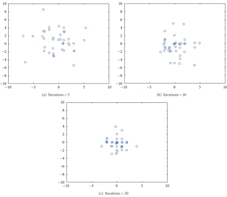
Figure 1: Population distribution observed at various stages in ABC.

noted that the value of𝑟_max and𝑟_min is set to0.8and0.3in ABC with LTVS in this experiment. Figures1and2show the population distribution at5th,10th, and20th iteration when the 2-dimensional Rastrigin function was optimized by the original ABC and ABC with LTVS, respectively. Compared with the original ABC, we can obtain that the population in ABC with LTVS distributed in a wider range of search space at a relatively small iteration and gradually gathered around the global optimum. In other words, LVTS can explore in the search space in the early search stage, while converging to the global optimum with fast speed in the later search.

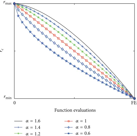
It would be interesting to know whether the nonlinear variation of 𝑟_𝑐 can enhance the performance of the ABC algorithm. In the preset study, we proposed a nonlinear-decreasing time-varying strategy (NTVS). This strategy is given as the following equation:

𝑟_𝑐= 𝑟_max− (𝑟_max− 𝑟_min) × (fitc FEs)

𝛼

, (6)

where𝛼is the nonlinear modulation index.Figure 3shows typical variations of𝑟_𝑐with function evaluations for different

settings of𝛼. With𝛼 = 1, this strategy becomes a special case of LTVS. With𝛼 > 1,𝑟_𝑐varied in a convex function manner. Compared with LTVS, it can be seen that𝑟_𝑐 decreases in a relative-slow speed in the early search while in a faster speed in the later search. Conversely, with𝛼 < 1,𝑟_𝑐 varied in a concave function manner.

3.2. Parameters Tuning of Time-Varying Strategy. In order to investigate the influence of 𝑟_max and 𝑟_min in LTVS, six combinations for setting the values of 𝑟_max and 𝑟_min are tested on8relevant functions including3typical unimodal functions,𝑓₁,𝑓₂, and𝑓₃, and5typical multimodal functions, 𝑓6,𝑓7,𝑓8,𝑓9, and𝑓10, with30dimensions. The colony size

(5)

−10 −5 0 5 10 −10

−8 −6 −4 −2 0 2 4 6 8 10

(a) Iterations = 5

−10 −5 0 5 10

−10 −8 −6 −4 −2 0 2 4 6 8 10

(b) Iterations = 10

−10 −5 0 5 10

−10 −8 −6 −4 −2 0 2 4 6 8 10

[image:5.600.189.411.495.715.2]

(c) Iterations = 20

Figure 2: Population distribution observed at various stages in ABC with time-varying strategy.

0 FEs

rmin

rmax

Function evaluations rc

𝛼 = 1.6 𝛼 = 1.4 𝛼 = 1.2

𝛼 = 1 𝛼 = 0.8 𝛼 = 0.6

(6)

[image:6.600.49.552.89.344.2]

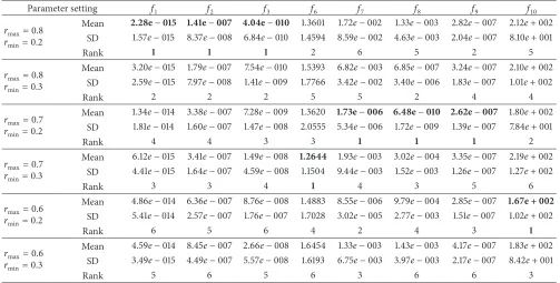
Table 1: Experimental results of different combination of𝑟_maxand𝑟_minin LTVS.

Parameter setting 𝑓₁ 𝑓₂ 𝑓₃ 𝑓₆ 𝑓₇ 𝑓₈ 𝑓₉ 𝑓₁₀

𝑟max= 0.8

𝑟min= 0.2

Mean 2.28e−015 1.41e−007 4.04e−010 1.3601 1.72e−002 1.33e−003 2.82e−007 2.12e+ 002 SD 1.57e−015 8.37e−008 6.84e−010 1.4594 8.59e−002 4.63e−003 2.04e−007 8.10e+ 001

Rank 1 1 1 2 6 5 2 5

𝑟_max= 0.8 𝑟min= 0.3

Mean 3.20e−015 1.79e−007 7.54e−010 1.5393 6.82e−003 6.85e−007 3.24e−007 2.10e+ 002 SD 2.59e−015 7.97e−008 1.41e−009 1.7766 3.42e−002 3.40e−006 1.83e−007 1.01e+ 002

Rank 2 2 2 5 5 2 4 4

𝑟_max= 0.7 𝑟_min= 0.2

Mean 1.34e−014 3.38e−007 7.28e−009 1.3620 1.73e−006 6.48e−010 2.62e−007 1.80e+ 002 SD 1.81e−014 1.60e−007 1.47e−008 2.0555 5.34e−006 1.72e−009 1.39e−007 7.84e+ 001

Rank 4 4 3 3 1 1 1 2

𝑟max= 0.7

𝑟_min= 0.3

Mean 6.12e−015 3.41e−007 1.49e−008 1.2644 1.93e−003 3.02e−004 3.35e−007 2.19e+ 002 SD 4.41e−015 1.64e−007 4.59e−008 1.1504 9.44e−003 1.52e−003 1.26e−007 1.27e+ 002

Rank 3 3 4 1 4 3 5 6

𝑟max= 0.6

𝑟min= 0.2

Mean 4.86e−014 6.36e−007 8.76e−008 1.4883 8.55e−006 9.79e−004 2.85e−007 1.67e + 002 SD 5.41e−014 2.57e−007 1.76e−007 1.7028 3.02e−005 2.77e−003 1.51e−007 1.02e+ 002

Rank 6 5 6 4 2 4 3 1

𝑟_max= 0.6 𝑟min= 0.3

[image:6.600.52.550.388.439.2]

Rank 5 6 5 6 3 6 6 3

Table 2: Rank results of the different combinations of𝑟_maxand𝑟_minin LTVS.

𝑟max= 0.8 𝑟max= 0.8 𝑟max= 0.7 𝑟max= 0.7 𝑟max= 0.6 𝑟max= 0.6

𝑟_min= 0.2 𝑟_min= 0.3 𝑟_min= 0.2 𝑟_min= 0.3 𝑟_min= 0.2 𝑟_min= 0.3

Average rank 2.875 3.25 2.375 3.625 3.875 5

Final rank 2 3 1 4 5 6

it shows that the settings of 𝑟_max = 0.7 and 𝑟_min = 0.2 are the best choice. Therefore, the parameters of𝑟_max = 0.7 and 𝑟_min = 0.2 are used in LTVS. We try to obtain better performance with the NTVS of𝛼 ̸= 1having𝑟_maxand𝑟_min kept fixed to their values obtained for the linear case.Table 3 shows the performance evaluation of the resultant system with different values of𝛼, keeping FEs = 7 × 104. From Tables3and4, we can observe that the best result is obtained with𝛼 = 1.2.

4. Experimental Study

4.1. Benchmark Functions and Parameters Settings. In order to test the proposed algorithm, a diverse set of21benchmark functions are used to conduct the experiments. These bench-mark functions can be classified into three groups: Group 1, Group 2, and Group 3. The first five functions𝑓₁–𝑓₅ are unimodal functions in Group 1. The next group includes ten multimodal functions with many local optima which are used to test the global search capability in avoiding premature con-vergence. Note that𝑓₆(Rosenbrock) is a unimodal problem in2D or3D search space but is a multimodal problem in

higher dimensions. Rotated and/or shifted functions belong to Group 3. 𝑓₁₆ and 𝑓₁₇ are rotated functions, in which the original variable ⃗𝑥 is rotated by left multiplying the orthogonal matrix 𝑀 [43], ⃗𝑦 = 𝑀 × ⃗𝑥. 𝑀 is used to increase the complexity of the function by changing separable functions to nonseparable functions without affecting the shape of the functions. The global optima of𝑓₁₈and𝑓₁₉are shifted to different numerical values for different dimensions ( ⃗𝑧 = ⃗𝑥 − ⃗𝑜), where ⃗𝑜is employed to shift the global optimal solution of the original function from the center of the search space to a new location.𝑓₂₀and𝑓₂₁are complicated which are shifted and rotated. We used ⃗𝑥∗to represent global optimum. In each benchmark function, ⃗𝑥∗and𝑓( ⃗𝑥∗)represent global optimum and the corresponding function value, respectively. The function value of the best solution found by an algorithm in a run is denoted by𝑓( ⃗𝑥best). The error of this run is denoted

as error= 𝑓( ⃗𝑥best) − 𝑓( ⃗𝑥∗). The parameters of all benchmark

functions are described in Appendix.

(7)

[image:7.600.52.552.88.402.2]

Table 3: Experimental results of different setting of𝛼in NTVS.

Parameter setting 𝑓₁ 𝑓₂ 𝑓₃ 𝑓₆ 𝑓₇ 𝑓₈ 𝑓₉ 𝑓₁₀

𝛼 = 1.6

Rank 3 2 4 3 5 6 5 5

𝛼 = 1.4

Mean 7.04e−018 2.36e−007 1.59e−012 1.6515 8.40e−010 6.48e−004 4.78e−009 1.41e+ 002 SD 6.61e−018 1.36e−007 3.38e−012 1.6594 2.33e−009 2.35e−003 2.83e−009 1.05e+ 002

Rank 2 3 1 5 2 5 1 2

𝛼 = 1.2

Mean 1.46e−018 4.76e−009 4.21e−012 1.5987 6.25e−010 1.01e−005 5.58e−009 9.60e + 001 SD 2.66e−018 3.43e−009 9.92e−012 1.4570 1.61e−009 4.69e−005 2.94e−009 8.84e+ 001

Rank 1 1 2 4 1 2 2 1

𝛼 = 1

Mean 1.34e−014 3.38e−007 7.28e−009 1.3620 1.73e−006 6.48e−010 2.62e−007 1.80e+ 002 SD 1.81e−014 1.60e−007 1.47e−008 2.0555 5.34e−006 1.72e−009 1.39e−007 7.84e+ 001

Rank 4 4 6 2 6 1 3 4

𝛼 = 0.8

Rank 5 5 3 1 4 4 4 6

𝛼 = 0.6

Rank 6 6 5 6 3 3 6 3

Table 4: Rank results of different setting of𝛼in NTVS.

𝛼 = 1.6 𝛼 = 1.4 𝛼 = 1.2 𝛼 = 1.0 𝛼 = 0.8 𝛼 = 0.6

Average rank 4.125 2.625 1.75 3.75 4 4.75

Final rank 5 2 1 3 4 6

for all algorithms and it is set to be7 × 104for solving30D problems and1.2×105for solving50D problems, respectively. The parameter,limit, is set to200[42]. All experiments on each benchmark function were run25times independently.

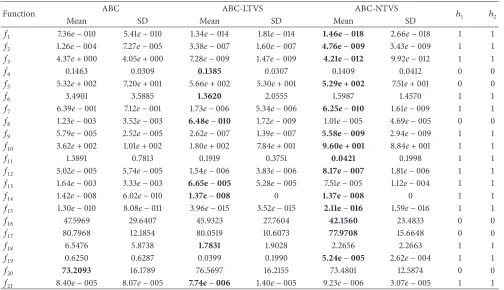
4.2. Experimental Results for 30D Problems. The comparative results obtained by ABC, ABC-LTVS, and ABC-NTVS are presented inTable 5. The best mean results on each problem among all algorithms are given in bold. In order to determine whether the results obtained by ABC-LTVS and ABC-NTVS are statistically different from the results generated by ABC algorithms, a two-tailed𝑡-test with 48 degrees of freedom is used at a significant level of 0.05. Values of “1,” “0,” and “−1” in columns “ℎ₁” and “ℎ₂” inTable 5, respectively, denote that ABC-LTVS and ABC-NTVS perform significantly better than, almost the same as, and significantly worse than ABC algorithm. In order to give visualized comparisons of the involved algorithms, the convergence graphs of the best and mean function values for each ABC algorithm regarding all

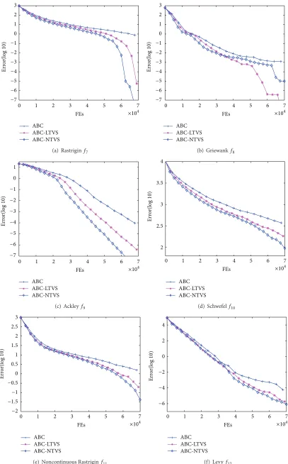
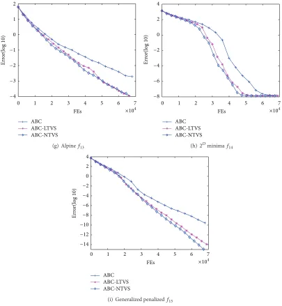
benchmark functions are shown in Figures 4, 5, and 6. In these figures, each curve represents the variation of mean value of error over the FEs for a specific ABC algorithm.

For solving unimodal functions, ABC-NTVS achieves the highest solution accuracy on𝑓₁,𝑓₂, 𝑓₃, and 𝑓₅, and ABC-LTVS obtains the best solution on𝑓₄. LTVS and ABC-NTVS perform significantly better than ABC algorithm on 𝑓1,𝑓2, and𝑓3. On multimodal problems, there are many local

minima and it is not easy to find the global optima. ABC-LTVS and ABC-NTVS are shown to offer better performance than ABC algorithm on these problems. ABC-LTVS can find the best solution on 𝑓₆, 𝑓₈, and 𝑓₁₃ and ABC-NTVS performs the best on𝑓₇,𝑓₉,𝑓₁₀,𝑓₁₁, and𝑓₁₂. ABC, ABC-LTVS, and ABC-NTVS obtain the similar performance on 𝑓₁₄. The performance of ABC-LTVS and ABC-NTVS are significantly better than that of ABC algorithm on these multimodal problems except ABC-NTVS for solving𝑓₈.

[image:7.600.59.550.446.485.2]

(8)

[image:8.600.50.554.88.378.2]

Table 5: Experimental results for 30-dimension problem.

Function ABC ABC-LTVS ABC-NTVS ℎ₁ ℎ₂

Mean SD Mean SD Mean SD

𝑓1 7.36e−010 5.41e−010 1.34e−014 1.81e−014 1.46e−018 2.66e−018 1 1

𝑓2 1.26e−004 7.27e−005 3.38e−007 1.60e−007 4.76e−009 3.43e−009 1 1

𝑓₃ 4.37e+ 000 4.05e+ 000 7.28e−009 1.47e−009 4.21e−012 9.92e−012 1 1

𝑓₄ 0.1463 0.0309 0.1385 0.0307 0.1409 0.0412 0 0

𝑓5 5.32e+ 002 7.20e+ 001 5.66e+ 002 5.30e+ 001 5.29e + 002 7.51e+ 001 0 0

𝑓₆ 3.4901 3.5885 1.3620 2.0555 1.5987 1.4570 1 1

𝑓₇ 6.39e−001 7.12e−001 1.73e−006 5.34e−006 6.25e−010 1.61e−009 1 1

𝑓8 1.23e−003 3.52e−003 6.48e−010 1.72e−009 1.01e−005 4.69e−005 0 0

𝑓₉ 5.79e−005 2.52e−005 2.62e−007 1.39e−007 5.58e−009 2.94e−009 1 1

𝑓₁₀ 3.62e+ 002 1.01e+ 002 1.80e+ 002 7.84e+ 001 9.60e + 001 8.84e+ 001 1 1

𝑓11 1.3891 0.7813 0.1919 0.3751 0.0421 0.1998 1 1

𝑓₁₂ 5.02e−005 5.74e−005 1.54e−006 3.83e−006 8.17e−007 1.81e−006 1 1

𝑓₁₃ 1.64e−003 3.33e−003 6.65e−005 5.28e−005 7.51e−005 1.12e−004 1 1

𝑓14 1.42e−008 6.02e−010 1.37e−008 0 1.37e−008 0 1 1

𝑓₁₅ 1.30e−010 8.08e−011 3.96e−015 3.52e−015 2.11e−016 1.59e−016 1 1

𝑓₁₆ 47.5969 29.6407 45.9323 27.7604 42.1560 23.4833 0 0

𝑓17 80.7968 12.1854 80.0519 10.6073 77.9708 15.6648 0 0

𝑓18 6.5476 5.8738 1.7831 1.9028 2.2656 2.2663 1 1

𝑓₁₉ 0.6250 0.6287 0.0399 0.1990 5.24e−005 2.62e−004 1 1

𝑓20 73.2093 16.1789 76.5697 16.2155 73.4801 12.5874 0 0

𝑓21 8.40e−005 8.07e−005 7.74e−006 1.40e−005 9.23e−006 3.07e−005 1 1

problems. Table 5 shows the results on the rotated and/or shifted functions. The results appear that these three ABC algorithms are affected. We can observe that ABC-LTVS and NTVS still obtain relatively good performance. ABC-LTVS and ABC-NTVS performs significantly better than ABC algorithms on 𝑓₁₈, 𝑓₁₉, and 𝑓₂₁. With respect to the stability of algorithms, ABC-LTVS and ABC-NTVS show the good stability as compared to ABC algorithms. The standard deviations of solutions found by ABC-LTVS and ABC-NTVS are small for the most functions. On the whole, ABC-LTVS and ABC-NTVS exhibit the accurate convergence precision on almost all the benchmark, which indicates the effec-tiveness of the proposed time-varying strategy. Moreover, experimental results demonstrate that ABC-NTVS slightly outperforms ABC-LTVS.

4.3. Experimental Results for 50D Problems. The experiments conducted on 50D problems and the results for solving unimodal, multimodal, and shift and/or rotate problems are presented in Table 6. As the convergence graphs of 50D are similar to the30D problems and space limitation, they are not given. Compared with ABC algorithm, ABC-LTVS and ABC-NTVS can still obtain high-quality solutions under50D problems, which can be seen fromTable 6. The meaning of column “ℎ₁” and “ℎ₂” in Table 6 is the same as theTable 5. It is noted that ABC-NTVS, from the mean of the results, performs worse than ABC on 𝑓₈, but not statistically significantly. According the𝑡-tests results, ABC-LTVS performs significantly better than ABC algorithm on

all benchmark functions except𝑓₄,𝑓₁₆, and𝑓₁₇, so does ABC-NTVS except𝑓₄,𝑓₈, and𝑓₁₇.

The experiments conducted on 50D problems and the results for solving unimodal, multimodal, and shift and/or rotate problems are presented inTable 6. As the convergence graphs of 50D are similar to the 30D problems and space limitation, they are not given. Compared with ABC algo-rithm, ABC-LTVS and ABC-NTVS can still obtain high-quality solutions under50D problems, which can be seen fromTable 6. The meaning of column “ℎ₁” and “ℎ₂” inTable 6 is the same as theTable 5. According to the𝑡-tests results, ABC-LTVS performs significantly better than ABC algorithm on all benchmark functions except𝑓₅,𝑓₁₆, and𝑓₁₇, so does ABC-NTVS except𝑓₅,𝑓₈, and𝑓₁₇.

(9)

0 1 2 3 4 5 6 7

×104

−15 −10 −5 0 5

FEs

Er

ro

r(log

10

)

(a) Sphere𝑓₁

0 1 2 3 4 5 6 7

×104

FEs

Er

ro

r(log

10

)

−8 −6 −4 −2 0 2 4 6 8 10 12

(b) Schwefel’s P2.22𝑓₂

0 1 2 3 4 5 6 7

×104

FEs

Er

ro

r(log

10

)

−6 −4 −2 0 2 4 6 8

(c) Elliptic𝑓3

0 1 2 3 4 5 6 7

×104

FEs

Er

ro

r(log

10

)

−1 −0.5 0 0.5 1 1.5 2

(d) Noise𝑓4

0 1 2 3 4 5 6 7

×104

FEs

Er

ro

r(log

10

)

ABC ABC-LTVS ABC-NTVS 2.7

2.8 2.9 3 3.1 3.2 3.3 3.4

(e) Zakharov𝑓₅

0 1 2 3 4 5 6 7

×104

FEs

Er

ro

r(log

10

)

ABC ABC-LTVS ABC-NTVS 0

0.5 1 1.5 2 2.5 3 3.5 4 4.5 5

(f) Rosenbrock𝑓₆

(10)

−7 −6 −5 −4 −3 −2 −1 0 1 2 3

0 1 2 3 4 5 6 7

×104

FEs

Er

ro

r(log

10

)

ABC ABC-LTVS ABC-NTVS

(a) Rastrigin𝑓7

0 1 2 3 4 5 6 7

×104

FEs −7

−6 −5 −4 −3 −2 −1 0 1 2 3

Er

ro

r(log

10

)

(b) Griewank𝑓8

0 1 2 3 4 5 6 7

×104

FEs −7

−6 −5 −4 −3 −2 −1 0 1

Er

ro

r(log

10

)

(c) Ackley𝑓₉

0 1 2 3 4 5 6 7

×104

FEs 2

2.5 3 3.5 4

Er

ro

r(log

10

)

(d) Schwefel𝑓₁₀

0 1 2 3 4 5 6 7

×104

FEs −2

−1.5 −1 −0.5 0 0.5 1 1.5 2 2.5 3

Er

ro

r(log

10

)

(e) Noncontinuous Rastrigin𝑓₁₁

0 1 2 3 4 5 6 7

×104

FEs −6

−4 −2 0 2 4

Er

ro

r(log

10

)

[image:10.600.97.504.71.725.2]

(f) Levy𝑓₁₂

(11)

0 1 2 3 4 5 6 7

×104

FEs −4

−3 −2 −1 0 1 2

Er

ro

r(log

10

)

(g) Alpine𝑓13

0 1 2 3 4 5 6 7

×104

FEs −8

−6 −4 −2 0 2 4

Er

ro

r(log

10

)

(h)2𝐷minima𝑓14

0 1 2 3 4 5 6 7

×104

FEs −14

−12 −10 −8 −6 −4 −2 0 2 4

Er

ro

r(log

10

)

[image:11.600.98.503.72.511.2]

(i) Generalized penalized𝑓15

Figure 5: Convergence curves of ABC variants solving multimodal functions𝑓₇–𝑓₁₅.

size and FEs, the settings of which is same as the previous experiment.

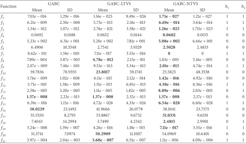
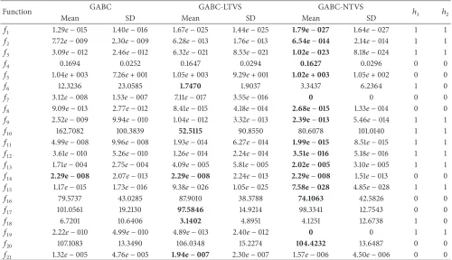
Tables 7 and 8 give the experimental results on 30D and 50D problems, respectively. The best results on each problem among these three GABC algorithms are shown in bold. In addition, the columns “ℎ₁” and “ℎ₂” in Tables 7 and 8 are used to determine the statistical significance of the difference obtained by GABC with those yielded by the GABC-LTVS and GABC-NTVS using two-tailed𝑡-tests, respectively. According to the results of 𝑡-tests shown in Tables7and8, GABC-LTVS and GABC-NTVS can find more accurate solutions, which are significantly better than those of GABC on about half of all benchmark functions regardless of problem dimensions.

5. Conclusions

(12)

0 1 2 3 4 5 6 7

×104

FEs 1.5

2 2.5 3 3.5 4 4.5 5 5.5 6 6.5 7

Er

ro

r(log

10

)

(a) Rotated Rosenbrock𝑓16

0 1 2 3 4 5 6 7

×104

FEs 1.8

2 2.2 2.4 2.6 2.8 3

Er

ro

r(log

10

)

(b) Rotated Rastrigin𝑓17

0 1 2 3 4 5 6 7

×104

FEs 0

1 2 3 4 5 6 7

Er

ro

r(log

10

)

(c) Shifted Rosenbrock𝑓18

0 1 2 3 4 5 6 7

×104

FEs −4

−3 −2 −1 0 1 2 3

Er

ro

r(log

10

)

(d) Shifted Rastrigin𝑓19

0 1 2 3 4 5 6 7

×104

FEs 1.8

2 2.2 2.4 2.6 2.8 3

Er

ro

r(log

10

)

(e) Shifted Rotated Rastrigin𝑓20

0 1 2 3 4 5 6 7

×104

FEs −5

−4 −3 −2 −1 0 1 2 3

Er

ro

r(log

10

)

(f) Shifted Rotated Griewank𝑓21

(13)

[image:13.600.50.550.101.390.2]

Table 6: Experimental results for 50-dimension problem.

Function ABC ABC-LTVS ABC-NTVS ℎ₁ ℎ₂

𝑓1 6.88e−010 3.54e−010 9.35e−015 7.24e−015 5.28e−016 5.79e−016 1 1

𝑓2 1.59e−004 9.94e−005 4.22e−007 2.01e−007 7.14e−008 2.67e−008 1 1

𝑓₃ 4.57e−005 6.75e−005 8.82e−008 3.58e−007 3.51e−010 4.42e−010 1 1

𝑓4 0.3606 0.0579 0.3132 0.0691 0.3214 0.0657 1 1

𝑓5 1.11e+ 003 1.09e+ 002 1.09e+ 003 9.64e+ 001 1.07e + 003 8.08e+ 001 0 0

𝑓₆ 8.2319 6.6280 1.3564 1.8842 1.3761 1.8716 1 1

𝑓7 1.0794 0.7609 0.0979 0.2829 0.0865 0.2755 1 1

𝑓8 2.45e−008 3.16e−008 1.42e−009 5.88e−009 3.23e−004 1.54e−003 1 0

𝑓₉ 4.78e−005 1.49e−005 2.25e−007 9.33e−008 5.01e−008 2.47e−008 1 1

𝑓₁₀ 7.83e+ 002 1.75e+ 002 3.97e+ 002 9.89e+ 001 3.45e + 002 1.78e+ 002 1 1

𝑓11 2.7273 0.9297 0.3388 0.4789 0.3029 0.4551 1 1

𝑓₁₂ 4.16e−005 7.77e−005 9.34e−007 2.42e−006 2.55e−007 6.02e−007 1 1

𝑓₁₃ 4.52e−003 4.91e−003 5.76e−004 7.16e−004 4.73e−004 5.83e−004 1 1

𝑓14 2.37e−008 1.33e−009 2.29e−008 1.40e−012 2.29e−008 1.07e−012 1 1

𝑓₁₅ 1.57e−010 1.41e−010 4.61e−015 4.07e−015 3.53e−016 4.77e−016 1 1

𝑓₁₆ 95.9988 40.0144 82.0768 32.2224 72.1410 26.1076 0 1

𝑓17 142.9558 23.9951 143.1200 18.8582 142.5459 20.4493 0 0

𝑓₁₈ 5.9388 4.7166 1.6944 1.7353 1.9040 1.8484 1 1

𝑓₁₉ 1.5057 0.8212 0.1243 0.3400 0.0400 0.1990 1 1

𝑓20 152.5097 18.9577 141.0244 20.0979 146.2151 17.2185 1 0

𝑓₂₁ 1.30e−004 2.39e−004 6.84e−006 8.96e−006 4.41e−006 5.53e−006 1 1

Table 7: Experimental results for 30D problem of GABC algorithms.

Function GABC GABC-LTVS GABC-NTVS ℎ₁ ℎ₂

𝑓₁ 7.03e−016 1.29e−016 1.16e−025 9.49e−026 1.71e−027 1.21e−027 1 1

𝑓2 6.21e−009 2.30e−008 5.73e−013 2.18e−013 6.69e−014 3.64e−014 1 1

𝑓₃ 1.34e−012 1.07e−012 2.76e−021 3.38e−021 1.26e−023 1.711e−023 1 1

𝑓₄ 0.0692 0.0188 0.0652 0.0144 0.0602 0.0155 0 0

𝑓5 5.23e+ 002 6.31e+ 001 5.20e+ 002 7.81e+ 001 5.08e + 002 6.66e+ 001 0 0

𝑓₆ 6.4906 10.3348 2.7541 3.9329 2.5028 2.4833 0 0

𝑓₇ 8.62e−011 1.58e−010 7.11e−017 3.55e−016 0 0 1 1

𝑓8 7.89e−004 3.87e−003 4.78e−012 2.13e−011 1.03e−005 5.16e−005 0 0

𝑓₉ 2.07e−009 7.48e−010 9.53e−013 3.34e−013 2.01e−013 4.74e−014 1 1

𝑓₁₀ 59.7836 70.9355 23.8017 59.1745 25.5825 48.3538 0 0

𝑓11 3.76e−009 1.02e−008 6.11e−015 2.12e−014 1.42e−016 4.92e−016 0 0

𝑓12 5.71e−010 1.38e−009 1.51e−013 6.85e−013 4.58e−016 8.36e−016 1 1

𝑓₁₃ 2.58e−005 3.20e−005 1.11e−005 1.82e−005 8.89e−006 2.03e−005 0 1

𝑓14 1.37e−008 2.23e−013 1.37e−008 2.32e−013 1.37e−008 2.17e−013 0 0

𝑓15 6.39e−016 1.15e−016 4.72e−026 4.33e−026 6.54e−028 6.60e−028 1 1

𝑓₁₆ 38.0229 23.1492 41.9666 26.0778 38.1041 23.7575 0 0

𝑓17 55.5550 8.2793 53.8867 9.6732 51.0331 9.6130 0 0

𝑓18 7.4043 14.2994 3.7490 4.2342 2.4815 2.9901 0 1

𝑓₁₉ 3.24e−008 1.59e−007 4.26e−016 1.18e−015 7.11e−017 3.55e−016 1 1

𝑓20 51.3741 7.0974 50.2909 11.1007 54.0969 10.6401 0 0

[image:13.600.52.548.439.729.2]

(14)

[image:14.600.50.550.89.377.2]

Table 8: Experimental results for 50D problem of GABC algorithms.

Function GABC GABC-LTVS GABC-NTVS ℎ₁ ℎ₂

𝑓₁ 1.29e−015 1.40e−016 1.67e−025 1.44e−025 1.79e−027 1.64e−027 1 1

𝑓2 7.72e−009 2.30e−009 6.28e−013 1.76e−013 6.54e−014 2.14e−014 1 1

𝑓3 3.09e−012 2.46e−012 6.32e−021 8.53e−021 1.02e−023 8.18e−024 1 1

𝑓₄ 0.1694 0.0252 0.1647 0.0294 0.1627 0.0296 0 0

𝑓5 1.04e+ 003 7.26e+ 001 1.05e+ 003 9.29e+ 001 1.02e + 003 1.05e+ 002 0 0

𝑓6 12.3236 23.0585 1.7470 1.9037 3.3437 6.2364 1 0

𝑓₇ 3.12e−008 1.53e−007 7.11e−017 3.55e−016 0 0 0 0

𝑓8 9.09e−013 2.77e−012 8.41e−015 4.18e−014 2.68e−015 1.33e−014 0 0

𝑓9 2.52e−009 9.94e−010 1.04e−012 3.32e−013 2.39e−013 5.46e−014 1 1

𝑓₁₀ 162.7082 100.3839 52.5115 90.8550 80.6078 101.0140 1 1

𝑓₁₁ 4.99e−008 9.96e−008 1.93e−014 6.27e−014 1.99e−015 8.51e−015 1 1

𝑓12 3.61e−010 5.26e−010 1.26e−014 2.24e−014 3.51e−016 5.18e−016 1 1

𝑓₁₃ 1.71e−004 2.75e−004 4.09e−005 5.81e−005 2.02e−005 3.10e−005 1 1

𝑓₁₄ 2.29e−008 2.07e−013 2.29e−008 2.24e−013 2.29e−008 1.51e−013 0 0

𝑓15 1.17e−015 1.73e−016 9.38e−026 1.05e−025 7.58e−028 4.85e−028 1 1

𝑓₁₆ 79.5737 43.0285 87.9010 38.3788 74.1063 42.5826 0 0

𝑓₁₇ 101.0561 19.2130 97.5846 14.9214 98.3341 12.7543 0 0

𝑓18 6.7201 10.6406 3.1402 4.8951 4.1251 12.6738 1 0

𝑓₁₉ 2.22e−010 4.99e−010 4.89e−013 2.40e−012 0 0 1 1

𝑓₂₀ 107.1083 13.3490 106.0348 15.2274 104.4232 13.6487 0 0

𝑓21 1.32e−005 4.76e−005 1.94e−007 2.30e−007 1.57e−006 4.50e−006 0 0

applied in other state-of-the-art ABC variants to further improve the search performance.

Appendix

A. Benchmark Functions

A.1. Unimodal Functions

(1) Sphere function

𝑓₁( ⃗𝑥) =∑𝐷

𝑖=1

𝑥2_𝑖, −100 ≤ 𝑥_𝑖≤ 100, ⃗𝑥∗= {0}𝐷. (A.1)

(2) Schwefel’s function P2.22

𝑓₂( ⃗𝑥) =∑𝐷

𝑖=1󵄨󵄨󵄨󵄨𝑥𝑖󵄨󵄨󵄨󵄨 + 𝐷

∏

𝑖=1󵄨󵄨󵄨󵄨𝑥𝑖󵄨󵄨󵄨󵄨, −100 ≤ 𝑥𝑖

≤ 100, ⃗𝑥∗= {0}𝐷.

(A.2)

(3) Elliptic function

𝑓3( ⃗𝑥)

=∑𝐷

𝑖=1(10

6₎(𝑖−1)/(𝐷−1)_𝑥2

𝑖, −100 ≤ 𝑥𝑖≤ 100, ⃗𝑥∗= {0}𝐷.

(A.3)

(4) Noise function

𝑓4( ⃗𝑥) = 𝐷

∑

𝑖=1

𝑖𝑥4_𝑖 +random[0, 1) ,

−1.28 ≤ 𝑥_𝑖≤ 1.28, ⃗𝑥∗_{= {0}}𝐷_.

(A.4)

(5) Zakharov function

𝑓₅( ⃗𝑥) =∑𝐷

𝑖=1

𝑥2_𝑖 + (∑𝐷

𝑖=1

0.5𝑖𝑥_𝑖)

2

+ (∑𝐷

𝑖=1

0.5𝑖𝑥_𝑖)

4

,

−10 ≤ 𝑥_𝑖≤ 10, ⃗𝑥∗_{= {0}}𝐷_.

(A.5)

A.2. Multimodal Functions

(6) Rosenbrock function

𝑓₆( ⃗𝑥) =𝐷−1∑

𝑖=1

[100 (𝑥_𝑖+1− 𝑥2_𝑖)2+ (𝑥_𝑖− 1)2] ,

−30 ≤ 𝑥_𝑖≤ 30, ⃗𝑥∗= {1}𝐷.

(A.6)

(7) Rastrigin function

𝑓7( ⃗𝑥) = 𝐷

∑

𝑖=1(𝑥

2

𝑖 − 10cos(2𝜋𝑥𝑖) + 10) ,

− 10 ≤ 𝑥_𝑖≤ 10, ⃗𝑥∗_{= {0}}𝐷_.

(15)

(8) Griewank function

𝑓₈( ⃗𝑥) =₄₀₀₀1 ∑𝐷

𝑖=1

𝑥2

𝑖 −

𝐷

∏

𝑖=1

cos(𝑥𝑖 √𝑖) + 1, −600 ≤ 𝑥_𝑖≤ 600, ⃗𝑥∗= {0}𝐷.

(A.8)

(9) Ackley function

𝑓₉( ⃗𝑥) = −20exp(−0.2√1 𝐷

𝐷

∑

𝑖=1

𝑥2

𝑖) −exp(_𝐷1

𝐷

∑

𝑖=1

cos2𝜋𝑥_𝑖)

+ 20 + 𝑒, −32 ≤ 𝑥_𝑖≤ 32, ⃗𝑥∗_{= {0}}𝐷_.

(A.9)

(10) Schwefel function

𝑓₁₀( ⃗𝑥) = 418.9829 × 𝐷 −∑𝐷

𝑖=1

(𝑥_𝑖sin(√󵄨󵄨󵄨󵄨𝑥_𝑖󵄨󵄨󵄨󵄨)),

−500 ≤ 𝑥_𝑖≤ 500, ⃗𝑥∗= {420.96}𝐷.

(A.10)

(11) Noncontinuous Rastrigin function

𝑓₁₁( ⃗𝑥) =∑𝐷

𝑖=1

(𝑦_𝑖2− 10cos(2𝜋𝑦_𝑖) + 10) ,

−10 ≤ 𝑥_𝑖≤ 10, ⃗𝑥∗ = {0}𝐷,

(A.11)

where

𝑦_𝑖={{_{_{ {

𝑥_𝑖, 󵄨󵄨󵄨󵄨𝑥_𝑖󵄨󵄨󵄨󵄨 < 0.5, round(2𝑥_𝑖)

2 , 󵄨󵄨󵄨󵄨𝑥𝑖󵄨󵄨󵄨󵄨 ≥ 0.5, for 𝑖 = 1, 2, . . . , 𝐷.

(A.12)

(12) Levy function

𝑓₁₂( ⃗𝑥) =𝐷−1∑

𝑖=1

(𝑥_𝑖− 1)2[1 + 10sin2(3𝜋𝑥_𝑖+1)]

+sin2(3𝜋𝑥_𝑖) + 󵄨󵄨󵄨󵄨𝑥_𝐷− 1󵄨󵄨󵄨󵄨 [1 + 10sin2(3𝜋𝑥_𝐷)] ,

− 50 ≤ 𝑥_𝑖≤ 50, ⃗𝑥∗= {1}𝐷. (A.13)

(13) Alpine function

𝑓13( ⃗𝑥) = 𝐷

∑

𝑖=1󵄨󵄨󵄨󵄨𝑥𝑖

sin𝑥_𝑖+ 0.1𝑥_𝑖󵄨󵄨󵄨󵄨,

−10 ≤ 𝑥_𝑖≤ 10, ⃗𝑥∗ _{= {0}}𝐷_.

(A.14)

(14)2𝐷minima

𝑓₁₄( ⃗𝑥) = 78.332331408 × 𝐷 −∑𝐷

𝑖=1

(𝑥4_𝑖 − 16𝑥_𝑖2+ 5𝑥_𝑖) ,

−5 ≤ 𝑥_𝑖≤ 5, ⃗𝑥∗= {−2.9035}𝐷. (A.15)

(15) Generalized penalized

𝑓₁₅( ⃗𝑥) = _𝐷𝜋{10sin2(𝜋𝑦₁) +

𝐷−1

∑

𝑖=1

(𝑦_𝑖− 1)2

× [1 + 10sin2(𝜋𝑦_𝑖+1)] + (𝑦_𝐷− 1)2}

+∑𝐷

𝑖=1

𝑢 (𝑥_𝑖, 10, 100, 4)

− 50 ≤ 𝑥_𝑖≤ 50, ⃗𝑥∗= {1}𝐷, (A.16)

where

𝑦_𝑖= 1 + 1

4(𝑥𝑖+ 1) ,

𝑢 (𝑥_𝑖, 𝑎, 𝑘, 𝑚) = { { { { { { { { {

𝑘 (𝑥_𝑖− 𝑎)𝑚, 𝑥_𝑖> 𝑎, 0, −𝑎 < 𝑧_𝑖< 𝑎, 𝑘 (−𝑥𝑖− 𝑎)𝑚, 𝑥𝑖< −𝑎.

(A.17)

A.3. Shifted and Rotated Functions

(16) Rotated Rosenbrock function

𝑓₁₆( ⃗𝑥) =𝐷−1∑

𝑖=1

[100 (𝑦_𝑖+1− 𝑦_𝑖2)2+ (𝑦_𝑖− 1)2] ,

⃗𝑦 = 𝑀 × ⃗𝑥, −10 ≤ 𝑥𝑖≤ 10, ⃗𝑥∗= {0}𝐷.

(A.18)

(17) Rotated Rastrigin function

𝑓₁₇( ⃗𝑥) =∑𝐷

𝑖=1

[𝑦2_𝑖 − 10cos(2𝜋𝑦_𝑖) + 10] ,

⃗𝑦 = 𝑀 × ⃗𝑥, −5.12 ≤ 𝑥𝑖≤ 5.12, ⃗𝑥∗= {0}𝐷.

(A.19)

(18) Shifted Rosenbrock function

𝑓₁₈( ⃗𝑥) =𝐷−1∑

𝑖=1

[100 (𝑧_𝑖+1− 𝑧2_𝑖)2+ (𝑧_𝑖− 1)2] ,

⃗𝑧 = ⃗𝑥 − ⃗𝑜 + 1, −10 ≤ 𝑥𝑖≤ 10, ⃗𝑥∗ = {𝑜}𝐷.

(A.20)

(19) Shifted Rastrigin function

𝑓19( ⃗𝑥) = 𝐷−1

∑

𝑖=1 [𝑧

2

𝑖 − 10cos(2𝜋𝑧𝑖) + 10] ,

⃗𝑧 = ⃗𝑥 − ⃗𝑜, −5.12 ≤ 𝑥𝑖≤ 5.12, ⃗𝑥∗= {𝑜}𝐷.

(16)

(20) Shifted Rotated Rastrigin function

𝑓₂₀( ⃗𝑥) =𝐷−1∑

𝑖=1

[𝑧2

𝑖 − 10cos(2𝜋𝑧𝑖) + 10] ,

⃗𝑧 = ( ⃗𝑥 − ⃗𝑜) × 𝑀, −5.12 ≤ 𝑥𝑖≤ 5.12, ⃗𝑥∗= {𝑜}𝐷.

(A.22)

(21) Shifted Rotated Griewank function

𝑓₂₁( ⃗𝑥) = 1 4000

𝐷

∑

𝑖=1

𝑧_𝑖2−∏𝐷

𝑖=1

cos(𝑧𝑖 √𝑖) + 1,

⃗𝑧 = ( ⃗𝑥 − ⃗𝑜) × 𝑀, −600 ≤ 𝑥_𝑖≤ 600, ⃗𝑥∗= {0}𝐷. (A.23)

Conflict of Interests

The authors declare that there is no conflict of interests regarding the publication of this paper.

Acknowledgments

This work is partially supported by National Natural Science Foundation of China under Grant nos. 71240015, 71402103, and 61273367; National Science Foundation of SZU under Grant 836; the Foundation for Distinguished Young Talents in Higher Education of Guangdong, China, under Grant 2012WYM 0116; the MOE Youth Foundation Project of Humanities and Social Sciences at Universities in China under Grant 13YJC630123; The Youth Foundation Project of Humanities and Social Sciences in Shenzhen University under grant 14QNFC28; and Ningbo Science & Technology Bureau (Science and Technology Project no. 2012B10055).

References

[1] J. Kennedy, R. Eberhart, and Y. Shi,Swarm Intelligence, Morgan Kaufmann, Boston, Mass, USA, 2001.

[2] Y. Shi, “An optimization algorithm based on brainstorming process,”International Journal of Swarm Intelligence Research, vol. 2, no. 4, pp. 35–62, 2011.

[3] D. Karaboga, “An idea based on honey bee swarm for numer-ical optimization,” Tech. Rep., Erciyes University, Engineering Faculty, Computer Engineering Department, 2005.

[4] D. Karaboga and B. Akay, “A survey: algorithms simulating bee swarm intelligence,”Artificial Intelligence Review, vol. 31, no. 1– 4, pp. 61–85, 2009.

[5] D. Karaboga, B. Gorkemli, C. Ozturk, and N. Karaboga, “A comprehensive survey: artificial bee colony (ABC) algorithm and applications,”Artificial Intelligence Review, vol. 42, no. 1, pp. 21–57, 2014.

[6] D. Karaboga and B. Basturk, “A powerful and efficient algo-rithm for numerical function optimization: artificial bee colony (ABC) algorithm,”Journal of Global Optimization, vol. 39, no. 3, pp. 459–471, 2007.

[7] D. Karaboga, B. Akay, and C. Ozturk, “Artificial bee colony (ABC) optimization algorithm for training feed-forward neural networks,” inModeling Decisions for Artificial Intelligence, V. Torra, Y. Narukawa, and Y. Yoshida, Eds., vol. 4617 ofLecture Notes in Computer Science, pp. 318–329, Springer, Berlin, Ger-many, 2007.

[8] Q. Qin, S. Cheng, L. Li, and Y. Shi, “Artificial bee colony algorithm: a survey,”CAAI Transactions on Intelligent Systems, vol. 9, no. 2, pp. 127–135, 2014.

[9] W. Gao and S. Liu, “Improved artificial bee colony algorithm for global optimization,”Information Processing Letters, vol. 111, no. 17, pp. 871–882, 2011.

[10] M. S. Kiran and M. G¨und¨uz, “A recombination-based hybridization of particle swarm optimization and artificial bee colony algorithm for continuous optimization problems,” Applied Soft Computing Journal, vol. 13, no. 4, pp. 2188–2203, 2013.

[11] D. Karaboga and B. Akay, “A comparative study of artificial Bee colony algorithm,”Applied Mathematics and Computation, vol. 214, no. 1, pp. 108–132, 2009.

[12] C. Ozturk and D. Karaboga, “Hybrid artificial bee colony algorithm for neural network training,” inProceedings of the IEEE Congress of Evolutionary Computation (CEC ’11), pp. 84– 88, IEEE, June 2011.

[13] T.-J. Hsieh, H.-F. Hsiao, and W.-C. Yeh, “Forecasting stock mar-kets using wavelet transforms and recurrent neural networks: an integrated system based on artificial bee colony algorithm,” Applied Soft Computing Journal, vol. 11, no. 2, pp. 2510–2525, 2011.

[14] T.-J. Hsieh, H.-F. Hsiao, and W.-C. Yeh, “Mining financial dis-tress trend data using penalty guided support vector machines based on hybrid of particle swarm optimization and artificial bee colony algorithm,”Neurocomputing, vol. 82, pp. 196–206, 2012.

[15] R. Zhang, S. Song, and C. Wu, “A hybrid artificial bee colony algorithm for the job shop scheduling problem,”International Journal of Production Economics, vol. 141, no. 1, pp. 167–178, 2013. [16] A. Alvarado-Iniesta, J. L. Garcia-Alcaraz, M. I. Rodriguez-Borbon, and A. Maldonado, “Optimization of the material flow in a manufacturing plant by use of artificial bee colony algorithm,”Expert Systems with Applications, vol. 40, no. 12, pp. 4785–4790, 2013.

[17] Z. Cui and X. Gu, “An improved discrete artificial bee colony algorithm to minimize the makespan on hybrid flow shop problems,”Neurocomputing, vol. 148, pp. 248–259, 2015. [18] C. Zhang, D. Ouyang, and J. Ning, “An artificial bee colony

approach for clustering,”Expert Systems with Applications, vol. 37, no. 7, pp. 4761–4767, 2010.

[19] X. Yan, Y. Zhu, W. Zou, and L. Wang, “A new approach for data clustering using hybrid artificial bee colony algorithm,” Neurocomputing, vol. 97, pp. 241–250, 2012.

[20] M.-H. Horng, “Multilevel thresholding selection based on the artificial bee colony algorithm for image segmentation,”Expert Systems with Applications, vol. 38, no. 11, pp. 13785–13791, 2011. [21] M. He, K. Hu, Y. Zhu, L. Ma, H. Chen, and Y. Song,

“Hierar-chical artificial bee colony optimizer with divide-and-conquer and crossover for multilevel threshold image segmentation,” Discrete Dynamics in Nature and Society, vol. 2014, Article ID 941534, 22 pages, 2014.

[22] C. Zhang and B. Zhang, “A hybrid artificial bee colony algorithm for the service selection problem,”Discrete Dynamics in Nature and Society, vol. 2014, Article ID 835071, 13 pages, 2014. [23] K. Ayan and U. Kilic¸, “Artificial bee colony algorithm solution

for optimal reactive power flow,”Applied Soft Computing Jour-nal, vol. 12, no. 5, pp. 1477–1482, 2012.

(17)

[25] A. Banharnsakun, T. Achalakul, and B. Sirinaovakul, “The best-so-far selection in artificial bee colony algorithm,”Applied Soft Computing Journal, vol. 11, no. 2, pp. 2888–2901, 2011.

[26] Z.-A. He, C. Ma, X. Wang et al., “A modified artificial bee colony algorithm based on search space division and disruptive selection strategy,”Mathematical Problems in Engineering, vol. 2014, Article ID 432654, 14 pages, 2014.

[27] W.-F. Gao and S.-Y. Liu, “A modified artificial bee colony algorithm,”Computers & Operations Research, vol. 39, no. 3, pp. 687–697, 2012.

[28] W.-L. Xiang and M.-Q. An, “An efficient and robust artificial bee colony algorithm for numerical optimization,”Computers & Operations Research, vol. 40, no. 5, pp. 1256–1265, 2013. [29] A. Alizadegan, B. Asady, and M. Ahmadpour, “Two modified

versions of artificial bee colony algorithm,”Applied Mathematics and Computation, vol. 225, pp. 601–609, 2013.

[30] B. Akay and D. Karaboga, “A modified artificial bee colony algo-rithm for real-parameter optimization,”Information Sciences, vol. 192, pp. 120–142, 2012.

[31] K. Diwold, A. Aderhold, A. Scheidler, and M. Middendorf, “Per-formance evaluation of artificial bee colony optimization and new selection schemes,”Memetic Computing, vol. 3, no. 3, pp. 149–162, 2011.

[32] F. Kang, J. Li, and Z. Ma, “Rosenbrock artificial bee colony algo-rithm for accurate global optimization of numerical functions,” Information Sciences, vol. 181, no. 16, pp. 3508–3531, 2011. [33] B. Alatas, “Chaotic bee colony algorithms for global numerical

optimization,”Expert Systems with Applications, vol. 37, no. 8, pp. 5682–5687, 2010.

[34] W.-F. Gao, S.-Y. Liu, and L.-L. Huang, “A novel artificial bee colony algorithm based on modified search equation and orthogonal learning,”IEEE Transactions on Cybernetics, vol. 43, no. 3, pp. 1011–1024, 2013.

[35] Q. Qin, S. Cheng, Q. Zhang, Y. Wei, and Y. Shi, “Multiple strategies based orthogonal design particle swarm optimizer for numerical optimization,”Computers & Operations Research, vol. 60, pp. 91–110, 2015.

[36] S. Cheng, Y. Shi, and Q. Qin, “Promoting diversity in particle swarm optimization to solve multimodal problems,” inNeural Information Processing, B.-L. Lu, L. Zhang, and J. Kwok, Eds., vol. 7063 ofLecture Notes in Computer Science, pp. 228–237, Springer, Berlin, Germany, 2011.

[37] S. Cheng, Y. Shi, and Q. Qin, “Population diversity of particle swarm optimizer solving single and multi-objective problems,” International Journal of Swarm Intelligence Research, vol. 3, no. 4, pp. 23–60, 2012.

[38] S. Cheng,Population diversity in particle swarm optimization: definition, observation, control, and application [Ph.D. disserta-tion], Department of Electrical Engineering and Electronics, University of Liverpool, 2013.

[39] D. Karaboga and B. Akay, “A modified Artificial Bee Colony (ABC) algorithm for constrained optimization problems,” Applied Soft Computing Journal, vol. 11, no. 3, pp. 3021–3031, 2011.

[40] D. Karaboga and B. Basturk, “On the performance of artificial bee colony (ABC) algorithm,”Applied Soft Computing Journal, vol. 8, no. 1, pp. 687–697, 2008.

[41] A. Ratnaweera, S. K. Halgamuge, and H. C. Watson, “Self-organizing hierarchical particle swarm optimizer with time-varying acceleration coefficients,”IEEE Transactions on Evolu-tionary Computation, vol. 8, no. 3, pp. 240–255, 2004.

[42] T. K. Sharma and M. Pant, “Enhancing the food locations in an artificial bee colony algorithm,”Soft Computing, vol. 17, no. 10, pp. 1939–1965, 2013.

(18)

Submit your manuscripts at

http://www.hindawi.com

Hindawi Publishing Corporation

http://www.hindawi.com Volume 2014

Mathematics

Journal of

http://www.hindawi.com Volume 2014 Mathematical Problems in Engineering

Hindawi Publishing Corporation http://www.hindawi.com

Differential Equations

International Journal of

Volume 2014

http://www.hindawi.com Volume 2014 Hindawi Publishing Corporationhttp://www.hindawi.com Volume 2014

Mathematical PhysicsAdvances in

Complex Analysis

Journal of

Optimization

Journal of

Combinatorics

International Journal of Hindawi Publishing Corporation

Journal of

Function Spaces

Abstract and Applied Analysis

International Journal of Mathematics and Mathematical Sciences

Hindawi Publishing Corporation http://www.hindawi.com Volume 2014

The Scientific

World Journal

Discrete Dynamics in Nature and Society

http://www.hindawi.com Volume 2014 Hindawi Publishing Corporation

Discrete Mathematics

Journal of

http://www.hindawi.com Volume 2014 Hindawi Publishing Corporationhttp://www.hindawi.com Volume 2014

Artificial bee colony algorithm with time varying strategy

Research Article