warwick.ac.uk/lib-publications
Original citation:
Topping, P.M. & Yin, H. Ann. PDE (2017) 3: 6. doi:10.1007/s40818-017-0024-x
Permanent WRAP URL:
http://wrap.warwick.ac.uk/83303
Copyright and reuse:
The Warwick Research Archive Portal (WRAP) makes this work of researchers of the
University of Warwick available open access under the following conditions.
This article is made available under the Creative Commons Attribution 4.0 International
license (CC BY 4.0) and may be reused according to the conditions of the license. For more
details see:
http://creativecommons.org/licenses/by/4.0/
A note on versions:
The version presented in WRAP is the published version, or, version of record, and may be
cited as it appears here.
DOI 10.1007/s40818-017-0024-x
Sharp Decay Estimates for the Logarithmic Fast
Diffusion Equation and the Ricci Flow on Surfaces
Peter M. Topping1 · Hao Yin2
Received: 29 June 2016 / Accepted: 30 January 2017
© The Author(s) 2017. This article is published with open access at Springerlink.com
Abstract We prove the sharp localL1−L∞smoothing estimate for the logarithmic fast diffusion equation, or equivalently, for the Ricci flow on surfaces. Our estimate almost instantly implies an improvement of the knownLp−L∞estimate forp>1. It also has several applications in geometry, providing the missing step in order to pose the Ricci flow with rough initial data in the noncompact case, for example starting with a general noncompact Alexandrov surface, and giving the sharp asymptotics for the contracting cusp Ricci flow, as we show elsewhere.
Keywords Logarithmic fast diffusion equation·Ricci flow·Smoothing estimate
1 Introduction
Theorem 1.1 Suppose u: B× [0,T)→(0,∞)is a smooth solution to the equation
∂tu=logu (1.1)
on the unit ball B ⊂R2, and suppose that u0:=u(0)∈ L1(B). Then for allδ >0
(however small) and for any k ≥0and any time t ∈ [0,T)satisfying
t ≥ (u0−k)+L1(B)
4π (1+δ), we have supB1/2
u(t)≤C(t+k),
for some constant C<∞depending only on δ.
B
Peter M. Topping[email protected] http://www.warwick.ac.uk/~maseq/
1 Mathematics Institute, University of Warwick, Coventry CV4 7AL, UK
2 School of Mathematical Sciences, University of Science and Technology of China, Hefei 230026,
The theorem gives an interiorsupbound for the logarithmic fast diffusion equation, depending only on the initial data, andnoton the boundary behaviour ofu at later times. This is in stark contrast to the situation for the normal linear heat equation on the ball, whose solutions can be made as large at the origin as desired in as short a time as desired, whatever the initial datau0. We are crucially using the nonlinearity of the equation.
The theorem effectively provides anL1−L∞smoothing estimate. It has been noted [13] that noL1−L∞smoothing estimate should exist for this equation, because such terminology would normally refer to an estimate that gave an explicitsupbound in terms of t > 0 and u0L1, and this is impossible as we explain in Remark 1.7.
Our theorem circumvents this issue, and almost immediately implies the following improvement of the well-known Lp−L∞smoothing estimates for p > 1 (see in particular Davis-DiBenedetto-Diller [3] and Vázquez [13]) in which the constantCis universal, and in particular does not blow up asp↓1.
Theorem 1.2 Suppose u: B× [0,T)→(0,∞)is a smooth solution to the equation
∂tu =logu on the unit ball B ⊂R2, and suppose that u0 :=u(0)∈ Lp(B)for
some p >1. Then there exists auniversalC < ∞such that for any t ∈ (0,T)we have
sup
B1/2
u(t)≤C
t−1/(p−1)u0Lp/(p(pB−)1)+t
.
In fact, in Section4we will state and prove a slightly stronger result.
The key to understanding Theorem1.1, and to obtaining the sharpest statement, is to understand its geometric setting. That a Riemannian metricg =u.(d x2+d y2)
on the ballBevolves under the Ricci flow equation [8,9]∂tg = −2K g, whereK =
−1
2uloguis the Gauss curvature ofg, is equivalent to the conformal factorusolving
(1.1). Meanwhile, the unique complete hyperbolic metric (the Poincaré metric) has a conformal factor1
h(x):=
2 1− |x|2
2
,
and induces hyperbolic Ricci flows, or equivalently solutions of (1.1), given by(2t+
α)hfor arbitraryα∈R. Note here that the Gauss curvature ofhis given by
K = − 1
2hlogh ≡ −1. (1.2)
The sharp form of our main theorem asserts that an appropriate scaling of a hyper-bolic Ricci flow will eventually overtake any other Ricci flow, and will do so in a time that is determined only in terms of the distribution of area, relative to a scaled hyperbolic metric, of the initial data.
Theorem 1.3 Suppose u: B× [0,T)→(0,∞)is a smooth solution to the equation
∂tu=logu, with initial data u0:=u(0)on the unit ball B⊂R2, and suppose that
(u0−αh)+∈ L1(B)for someα ≥0. Then for allδ >0(however small) and any time t∈ [0,T)satisfying
t ≥ (u0−αh)+L1(B)
4π (1+δ), we have
sup
B
u(t)
h ≤2t+C
α+ (u0−αh)+L1(B)
,
where C<∞depends only onδ.
In other words, if we define αˆ := Cα+ (u0−αh)+L1(B)
, then u(t)will be overtaken by the self-similar solution(2t+ ˆα)hafter a definite amount of time.
Remark 1.4 To fully understand Theorem 1.3, it is important to note the geometric invariance of all quantities. In general, given a Ricci flow defined on a neighbourhood of some point in some surface, one can choose local isothermal coordinates near to the point in many different ways, and this will induce different conformal factors. However, the ratio of two conformal factors, for example u(ht),isinvariantly defined. In particular, if the flow is pulled back by a Möbius diffeomorphism B → B (i.e. an isometry ofBwith respect to the hyperbolic metric, which thus leaveshinvariant but changesuin general) then the supremum of this ratio is unchanged. Similarly, the quantity(u0−αh)+L1(B)is invariant under pulling back by Möbius maps, which
is instantly apparent by viewing it as theL1norm of the invariant quantity(u0
h −α)+
with respect to the (invariant) hyperbolic metric rather than the Euclidean metric.
Remark 1.5 An immediate consequence of Remark1.4(and the fact that one can pick a Möbius diffeomorphism mapping an arbitrary point to the origin) is that to control the supremum of u(ht)over the whole ballB, we only have to control it at the origin.
Remark 1.6 Continuing Remark 1.4, it is also convenient to note that the theorem really only requires a Ricci flow on a Riemann surface conformal to a disc in order to apply. This surface then admits a unique complete hyperbolic metric, and all quantities make sense without the need to explicitly pull back to the underlying disc. We will take this viewpoint when we are already considering a Ricci flow on a disc B, but wish to apply the theorem on some smaller sub-ball, for example on Bρ where the hyperbolic metric has larger conformal factor
hρ(x)= 1
ρ2h
x
ρ
as graphed in Fig.1.
Fig. 1 Conformal factors of hyperbolic metricshonBand
hρonBρ
r
h
h
ρ−1 ρ ρ 1
To see that Theorem1.1follows from Theorem1.3, for our givenkwe setα=k/4. Thenαh ≥konB, so(u0−k)+≥(u0−αh)+, and any time valid in Theorem1.1 will also be valid in Theorem1.3, i.e.
t≥ (u0−k)+L1(B)
4π (1+δ) ⇒ t≥
(u0−αh)+L1(B)
4π (1+δ).
We can deduce that
u(t)≤2t+Cα+ (u0−αh)+L1(B)
h
≤C(t+k)h, (1.3)
onB, and restricting toB1/2, whereh≤64/9, completes the proof.
Remark 1.7 To see that Theorem1.1is sharp, consider the so-called cigar soliton flow metric defined onR2by
˜
u(x,t)= 1 e4t + |x|2,
which solves (1.1). This is a so-called steady soliton, meaning that the metric at time
t = 0 is isometric to the metric at any other time t (here via the diffeomorphism
x → e2tx). Geometrically, the metric looks somewhat like an infinite half cylinder with the end capped off. It is more convenient to consider the scaled version of this solution given by
u(x,t)= 4
[image:5.439.192.388.62.242.2]forμ >0 small. The scaling is chosen here so thatu0L1(B)=4π, and thus Theorem
1.1tells us that if we wait until timet =1+δ, then we obtain a bound onu(0,t)(for example) that only depends onδ, and notμ. However, we see that
u(0,1−δ)= 4
log(μ−1+1)(1+μ)1−δμδ → ∞,
asμ↓ 0, for fixedδ >0 (however small), so no such upper bound is available just
beforethe special timet =1.
Note that for eacht ∈ [0,1), in the limitμ↓0 we have
u(x,t)→4π(1−t)δ0
as measures, whereδ0represents the delta function at the origin. This connects with
the discussion of Vázquez [14].
Remark 1.8 In [12], we apply Theorem1.3to give the sharp asymptotics of the con-formal factor of the contracting cusp Ricci flow as constructed in [10]. As a result, we obtain the sharp decay rate for the curvature as conjectured in [10].
2 Proof of the Main Theorem
In this section, we prove Theorem1.3, which implies Theorem1.1as we have seen. The proof will involve considering a potential that is an inverse Laplacian of the solu-tionu. Note that this is different from the potential considered by Hamilton and others in this context, which is an inverse Laplacian of the curvature. Indeed, the curvature arises from the potential we consider by application of afourthorder operator. Nev-ertheless, our potential can be related to the potential considered in Kähler geometry. Our approach is particularly close to that of [7], from which the main principles of this proof are derived. In contrast to that work, however, our result is purely local, and will equally well apply to noncompact Ricci flows.
The main inspiration leading to the statement of Theorem1.1was provided by the examples constructed by the first author and Giesen [5,6].
2.1 Reduction of the Problem
In this section, we successively reduce Theorem1.3to the simpler Proposition2.2. Consider first, form≥0,α≥0, the following assertion.
AssertionPm,α: For eachδ ∈ (0,1], there exists C < ∞ with the following
property. For each smooth solutionu : B× [0,T)→(0,∞)to the equation∂tu =
loguwith initial datau0:=u(0)on the unit ballB⊂R2, if
then
u(t0)≤C(m+α)h throughoutB, at timet0= m
4π(1+δ),
providedt0<T.
Claim 1 Theorem1.3follows if we establish{Pm,α}for everym≥0,α≥0.
Proof of Claim1 First observe that we may as well assumeδ∈(0,1]in the theorem, since the cases thatδ >1 follow from the caseδ =1. Takeαfrom the theorem and set
m= (u0−αh)+L1(B). AssertionPm,αtells us thatu(t0)≤C(m+α)hthroughout
Bat timet0=4mπ(1+δ)(unlesst0≥T, in which case there is nothing to prove). But
t →(2t+C(m+α))h
is the maximally stretched Ricci flow starting at C(m+α)h (i.e. it is the unique complete Ricci flow starting with this initial data, and thus agrees with the maximal flow that lies above any other solution [4,11]) and thus
u(t)≤(2(t−t0)+C(m+α))h ≤(2t+C(m+α))h (2.1)
for allt ≥t0, as desired.
It remains to prove the assertionsPm,α, but first we make some further reductions.
To begin with, we note that the assertionsP0,αare trivial, becauseu0≤αhandt0=0
in that case, so we may assume thatm>0.
By parabolic rescaling by a factorλ >0, more precisely by replacinguwithλu,
u0withλu0, andtwithλt, we see that in factPm,αis equivalent toPλm,λα. Thus, we
may assume, without loss of generality, thatm=1 and prove only the assertionsP1,α
for eachα≥0.
Next, it is clear that assertionP1,1 impliesP1,α for everyα ∈ [0,1]. Indeed, in
the setting of P1,α (α ≤ 1), we can apply assertionP1,1 to deduce that u(t0) ≤ C(1+1)h≤(2C)(1+α)h.
What is a little less clear is:
Claim 2 AssertionP1,1impliesP1,αfor everyα≥1.
Proof of Claim2 By the invariance of the assertionP1,αunder pull-backs by Möbius
maps (see Remark1.5), it suffices to prove thatu(t0)≤C(1+α)hat the origin inB, wheret0= 41π(1+δ). This in turn would be implied by the assertionu(t0)≤C hα−1/2
at the origin inB.
The assumption(u0−αh)+L1(B) ≤1 implies(u0−hα−1/2)+L1(B
α−1/2) ≤1
because
hα−1/2(x)=α.h
(recallα≥ 1). Therefore we can invokeP1,1on Bα−1/2 (cf. Remark1.6) to deduce
that
u(t0)≤C hα−1/2
at the origin as required.
Thus our task is reduced to proving that AssertionP1,1holds.
Keeping in mind Remark1.5again, we are reduced to proving:
Proposition 2.1 For each smooth solution u:B× [0,T)→(0,∞)to the equation
∂tu=logu with initial data u0:=u(0), if
(u0−h)+L1(B)≤1, (2.2)
then for eachδ ∈(0,1], we have
u(t0)≤C.h at the origin, at time t0= 1
4π(1+δ), (2.3)
provided t0<T , where C depends only onδ.
In this proposition, we make no assumptions on the growth ofu near∂Bother than what is implied by (2.2). However, we may assume without loss of generality that
u(t)is smooth up to the boundary∂B. To get the full assertions, we can apply this apparently weaker case on the restrictions of the flow toBρ, forρ ∈(0,1), and then letρ↑1. (Recall Remark1.6.)
Instead of estimatingu(t), we will estimate a larger solutionv(t)of the flow arising as follows. We would like to define new initial datav0onBby
v0(x):=max{u0(x),h(x)},
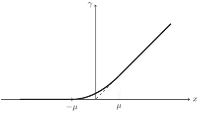
and then solve forwards in time to givev(t). This is certainly possible, but it will be technically simpler to consider a smoothed out (and even larger) version of this. Indeed, for eachμ >0 (however small) consider a smooth functionγ :R→ [0,∞) such thatγ (x)=0 forx≤ −μ,γ (x)=xforx≥μ, andγ≥0, as in Fig.2.
We can then consider instead the smooth function
v0(x):=h(x)+γ (u0(x)−h(x)). (2.4)
Thus we have v0 ≥ h,v0 ≥ u0, and in some neighbourhood of∂B,v0 = h.
Moreover, by takingμsufficiently small (depending onδ) we can be sure that
v0−hL1(B)≤ (u0−h)+L1(B)+ δ
100 ≤1+ δ 100.
Fig. 2 Smoothing functionγ γ
x
−μ μ
This flow will have bounded curvature, not just initially, but for all time, because v0≤C hfor some largeC(see [4], in contrast to [6]). Moreover, that solution will be
maximally stretched [4] and in particular, we will have
u(t)≤v(t) for allt∈ [0,T), and(2t+1)h≤v(t) for allt∈ [0,∞).
We see then that we are reduced to proving the following proposition, which will be the objective of the remainder of Section2.
Proposition 2.2 Supposev0:B →(0,∞)is smooth, withv0≥h and with equality outside a compact set in B. Suppose further that for someδ ∈(0,1]we have
v0−hL1(B) ≤1+ δ
100. (2.5)
Ifv : B× [0,∞)→ (0,∞)is the unique complete solution to the equation∂tv =
logvwith initial datav0:=v(0)(see[4,11]), then
v(t0)≤C at the origin, at time t0= 1
4π(1+δ), (2.6)
where C depends only onδ.
2.2 The Potential Function and the Differential Harnack Estimate
To prove Proposition2.2, we consider a potential function that will be constructed using the following lemma, which will be proved in Section3along with other technical aspects of the proof.
Lemma 2.3 Supposev0 : B → (0,∞)is smooth, withv0 ≥ h and with equality outside a compact set in B, and letv:B× [0,∞)→(0,∞)be the unique complete solution to the equation∂tv=logvwithv(0)=v0. Then there existsψ∈C∞(B×
[0,∞))∩C0(B× [0,∞))such that for all t≥0, we have
ψ(t)=v(t)−(2t+1)h
[image:9.439.188.387.61.176.2]and
∂tψ=logv−logh−log(2t+1). (2.8)
We can then define the potential function
ϕ=ψ+(t+1/2)log[(2t+1)h]. (2.9)
It is straightforward to check, using Lemma2.3and (1.2), that
ϕ=v, (2.10)
and
∂tϕ=logϕ+1. (2.11)
Following [7], we define the Harnack quantityH:B× [0,T)→Rto be
H:=tlogϕ−[ϕ(t)−ϕ(0)] (2.12)
=t∂tϕ−t−[ϕ(t)−ϕ(0)]. (2.13)
Lemma 2.4 Writingv := v1for the Laplacian with respect to the metric corre-sponding tov, we have
∂tH≤ vH, (2.14)
and
H≤0 (2.15)
throughout B× [0,∞).
Remark 2.5 ClearlyH(0)≡0, so the proof of this lemma, which we give in Section3, will involve verifying the equation forHand then checking that the maximum principle applies. Of course, one must take care about howHbehaves as we approach∂B, but rewritingHin terms ofψandvrather thanϕ, using (2.10) and (2.9) gives
H=tlog
v (2t+1)h
−[ψ(t)−ψ(0)]+1 2log
1 2t+1
, (2.16)
and we will show in Lemma3.1that
v
soHextends continuously to∂B, where it takes the value
H|∂B ≡
1 2log
1 2t+1
≤0,
so it seems reasonable to hope thatH≤ 0 holds. In fact, because the heat equation (2.14) satisfied byHinvolves the Laplacianv rather than, only a mild growth condition on the positive part ofHis required to make the maximum principle work, and in particular, it will suffice thatHis bounded above onB×[0,T], for eachT >0, rather than nonpositive at the boundary.
We end this section by noting the consequences of the Harnack Lemma2.4forv. Only the first, simpler, estimate will be required, but it will be required twice.
Corollary 2.6 In the setting of Lemma2.3, for all t>0we have
v(t)
(2t+1)h ≤exp
1−ψ(0)
t
(2.17)
or more generally
v(t)
(2t+1)h ≤(1+2t)
1/(2t)exp
ψ(
t)−ψ(0)
t
. (2.18)
The stronger statement (2.18) is nothing more than a rearrangement of (2.16) and the inequality H ≤ 0. The weaker statement (2.17) then follows by recalling that (1+1/x)x ≤efor allx>0, and noting that the equation (2.7) forψimpliesψ≥0 onB, withψ=0 on∂B, so the maximum principle implies thatψ(t)≤0.
2.3 Exponential Integrability
Continuing with the proof of Proposition2.2, recall that
ψ(0)=v0−h ≥(u0−h)+≥0,
by (2.4). We use the following theorem of Brezis and Merle [1].
Theorem 2.7 Supposeη∈W01,1(B)is a weak solution of
η= f ∈L1 on B;
η=0 on ∂B.
Then for0<p<4π/f1, we have
B
In particular, providedf1<4π, we obtain Lpcontrol one|η|for somep >1. We would like to apply this withη=ψ(0)/tand f = v0−t h, in which case hypothesis (2.5) of Proposition2.2tells us that
f1=v0−h1
t ≤
1
t
1+ δ 100
.
Therefore, ift > 41π(1+ 100δ )then we obtain Lpcontrol of the right-hand side of (2.17), for 1< p< 4πt
1+100δ .
To prove Proposition2.2, we need to obtain pointwise estimates onv(t)at time
t0= 41π(1+δ), but to do that, we first apply what we have just learned from Theorem 2.7at timet˜:= 41π(1+δ/2). This then gives us Lpcontrol in (2.17) for 1< p <
4πt˜
1+δ/100 = 1+δ/2
1+δ/100, and in particular we can set p=1+δ/3, and conclude that
B
exp
−pψ(˜0) t
≤C(δ),
or by (2.17) of Corollary2.6,
(2t˜v(+t˜)1)h
Lp(B)≤
C(δ). (2.19)
We now wish to bootstrap our Lpcontrol toL∞control. In order to do this, we view the Ricci flow as starting at timet˜, with initial datav(t˜)controlled as above, and repeat the construction of the potential function, Harnack quantity, and subsequent application of Corollary2.6, starting at this time. However, instead of using the Brezis-Merle Theorem2.7, we exploit our newLpcontrol in order to apply classical Calderon-Zygmund estimates instead. When making that step, the unboundedness ofhnear the boundary∂Bwould cause a problem; we avoid this by working only on the interior ballB1/2and comparing the flow with the hyperbolic metrich1/2. Or equivalently, we
make a rescaling of the domain coordinates so that the ballB1/2becomes a unit ball.
Following this second presentation, we defineu0˜ : B→(0,∞)by
˜
u0(x):= 1
4v(x/2,t˜),
and note that
˜
u(x,t):=1
4v(x/2,t˜+t),
is a subsequent (incomplete Ricci flow) solution on B for t ≥ 0. Our objective of proving the bound (2.6) would then be implied by a bound
˜
u(0,t0˜)≤C at timet0˜ :=t0− ˜t= δ
Unravelling (2.19) tells us that ˜u0Lp(B) ≤ C(δ). As before, we would like to define
˜
v0(x):=max{ ˜u0(x),h(x)},
but instead take the slight smoothing
˜
v0(x):=h(x)+γ (u0˜ (x)−h(x))
as in Section2.1and Fig.2. By choosingμ∈(0,1]for ourγ, we can be sure that
0≤ ˜v0−h≤1+ ˜u0. (2.21)
We can then apply Corollary2.6withv˜0in place ofv0 in order to estimate the
subsequent flowv(˜ t)≥ ˜u(t)by
˜
v(t)
(2t+1)h ≤exp
1−ψ(˜ 0)
t
, (2.22)
where, of course,
˜ψ(0)= ˜v0−h ˜
ψ(0)|∂B=0.
(2.23)
However, instead of applying Theorem2.7of Brezis-Merle to estimateψ(˜ 0), we apply Calderon-Zygmund theory. Equation (2.23) and the estimate (2.21) give
ψ(˜ 0)Lp(B)= ˜v0−hLp(B)≤ 1+ ˜u0Lp(B)≤C(δ).
Appealing to the zero boundary data tells us that
˜ψ(0)L∞(B) ≤C ˜ψ(0)W2,p(B)≤Cψ(˜ 0)Lp(B)≤C(δ),
and applying this to (2.22) at the origin, at timet0˜ :=t0− ˜t =8δπ gives
˜
v(0,t0˜)≤C
and hence (2.20), becauseu˜(t)≤ ˜v(t).
3 Proofs of Lemmas
Lemma 3.1 Forv0andvas in Lemma2.3, we have
v(t)
(2t+1)h(x)→1
uniformly as(x,t)→∂B× [0,∞).
Assuming for the moment that Lemma3.1is true, we give a proof of Lemma2.3.
Proof Instead of definingψ(t)by (2.7) and checking (2.8), we define onlyψ(0)by (2.7), i.e. we takeψ(0)to be the solution to
ψ(0)=v0−h
ψ(0)|∂B=0, (3.1)
which will be smooth (even up to the boundary) and then we extendψtot >0 by asserting (2.8), i.e. we define
ψ(t)=ψ(0)+
t
0 ∂
tψ(s)ds=ψ(0)+
t
0
log v(s) (2s+1)hds.
Basic ODE theory tells us thatψ∈C∞(B× [0,∞)). We also see thatψ∈C0(B× [0,∞)), withψ(t)|∂B ≡0 because
∂tψ(x,t)→0 uniformly as(x,t)→∂B× [0,∞)
by Lemma3.1.
It remains to check the first part of (2.7), i.e. that
ψ(t)=v(t)−(2t+1)h.
For that purpose, we compute
∂t(ψ)= (∂tψ)
= logv− logh =∂tv−2h
=∂t(v−(2t+1)h),
where we used (2.8), the PDE satisfied byv, and (1.2). Since we knowψ(0)=v(0)−h, we have
ψ(t)=v(t)−(2t+1)h
Proof of Lemma3.1 By assumption, we know thatv0≥honB, and that there exists a∈(0,1)such that on the annulus B\Bawe have
v0=h<h0:=
1
r(−logr) 2
<ha:=
⎡
⎣ π
(−loga)rsin
π(−logr)
−loga
⎤ ⎦ 2
,
whereh0andhaare the conformal factors of the unique complete conformal hyperbolic
metrics onB\{0}andB\Barespectively. These inequalities can be computed directly
(for example using that sin(x) <xforx∈(0, π)) though they follow instantly from the maximum principle, which tells us that when we reduce the domain, the hyperbolic metric must increase.
The unique complete solutionv(t)starting atv0is maximally stretched onB, and
so(2t+1)h ≤v(t), while onB\Ba, the solution(2t+1)ha, being complete, must
also be maximally stretched and so v(t) ≤ (2t +1)ha on this annulus (see [11]).
Therefore, we conclude that for allt ≥0, we have
1≤ v(t) (2t+1)h ≤
ha
h = ⎡
⎣ π(1−r2)
2(−loga)rsin
π(−logr)
−loga
⎤ ⎦ 2
→1
uniformly asr ↑1 as required.
We now prove the Harnack Lemma 2.4, but first we need to carefully state an appropriate maximum principle, which follows (for example) from the much more general [2, Theorem 12.22] using the Bishop-Gromov volume comparison theorem.
Theorem 3.2 Suppose g(t)is a smooth family of complete metrics defined on a smooth manifold M of any dimension, for0 ≤ t ≤ T , with Ricci curvature bounded from below and|∂tg| ≤C on M× [0,T].
Suppose f(x,t)is a smooth function defined on M× [0,T]that is bounded above and satisfies
∂tf ≤ g(t)f.
If f(x,0)≤0for all x∈ M, then f ≤0throughout M× [0,T].
Proof of Lemma2.4 Direct computation using (2.12), (2.10) and (2.11) shows that
∂tH=logϕ+t∂tϕ
ϕ −∂tϕ(t)
= −1+t∂tϕ
v , (3.2)
while computing using (2.13) gives
and hence from (2.10) we find that
vH=t∂tϕ
v −1+ v0
v .
Combining with (3.2) gives
∂tH−vH= −v0
v ≤0,
as required.
Letg(t)be the family of smooth metrics corresponding tov(t). Since we know the curvature ofg(t)is bounded, it satisfies the assumptions in Theorem3.2. Moreover, as discussed in Remark2.5,His bounded and equals zero initially, so Theorem3.2
then implies thatH≤0 for allt ≥0.
4
L
p−
L
∞Smoothing Results
In this section, we prove the following result that implies Theorem 1.2by setting 1+δ=4π.
Theorem 4.1 Suppose u:B×[0,T)→(0,∞)is a smooth solution to the equation
∂tu =logu
on the unit ball B ⊂R2, and suppose that u0:=u(0)∈Lp(B)for some p>1. Then
for allδ >0, there exists C =C(δ) <∞such that for any t∈(0,T)we have
sup
B1/2
u(t)≤C
4πt
1+δ
−1/(p−1)
u0p/(p−1)
Lp(B) +t
. (4.1)
Proof First suppose thatt ≥ u0L1(B)
4π (1+δ). Then Theorem1.1applies withk=0
to give
sup
B1/2
u(t)≤Ct,
which is stronger than (4.1). If instead we have t < u0L1(B)
4π (1+δ), then we can findk ≥ 0 such that t =
(u0−k)+L1(B)
4π (1+δ), and then apply Theorem1.1to find that
sup
B1/2
In order to estimatekin terms oft, we compute
u0p Lp(B)≥
{u0≥k}
u0p≥kp−1(u0−k)+L1(B)=kp−1
4πt
1+δ
and thus
k≤
4πt
1+δ
− 1
p−1
u0p−p1
Lp(B),
which when substituted into (4.2) gives the result.
Acknowledgements The first author was supported by EPSRC Grant No. EP/K00865X/1 and the second author was supported by NSFC 11471300.
Open Access This article is distributed under the terms of the Creative Commons Attribution 4.0 Interna-tional License (http://creativecommons.org/licenses/by/4.0/), which permits unrestricted use, distribution, and reproduction in any medium, provided you give appropriate credit to the original author(s) and the source, provide a link to the Creative Commons license, and indicate if changes were made.
References
1. Brezis, H., Merle, F.: Uniform estimates and blow-up behavior for solutions of−u=V(x)euin two dimensions. Commun. Partial Differ. Equ.16, 1223–1253 (1991)
2. Chow, B., Chu, S.C., Glickenstein, D., Guenther, C., Isenberg, J., Ivey, T., Knopf, D., Lu, P., Luo, F., Ni, L.: The Ricci Flow: Techniques and Applications: Part II: Analytic Aspects. Mathematical Surveys and Monographs, vol. 144. AMS (2008)
3. Davis, S.H., DiBenedetto, E., Diller, D.J.: Some a priori estimates for a singular evolution equation arising in thin-film dynamics. SIAM J. Math. Anal.27, 638–660 (1996)
4. Giesen, G., Topping, P.M.: Existence of Ricci flows of incomplete surfaces. Commun. Partial Differ. Equ.36, 1860–1880 (2011)
5. Giesen, G., Topping, P.M.: Ricci flows with unbounded curvature. Math. Zeit.273, 449–460 (2013) 6. Giesen, G., Topping, P.M.: Ricci flows with bursts of unbounded curvature. Commun. Partial Differ.
Equ.41, 854–876 (2016)
7. Guedj, V., Zeriahi, A.: Regularizing properties of the twisted Kähler–Ricci flow. To appear, J. Reine Angew. Math
8. Hamilton, R.S.: Three-manifolds with positive Ricci curvature. J. Differ. Geom.17, 255–306 (1982) 9. Topping, P.M.: Lectures on the Ricci flow. L.M.S. Lecture Notes Series, vol. 325. C.U.P., Cambridge
(2006).http://www.warwick.ac.uk/~maseq/RFnotes.html
10. Topping, P.M.: Uniqueness and nonuniqueness for Ricci flow on surfaces: reverse cusp singularities. Int. Math. Res. Not.2012, 2356–2376 (2012).arXiv:1010.2795
11. Topping, P.M.: Uniqueness of instantaneously complete Ricci flows. Geom. Topol.19, 1477–1492 (2015)
12. Topping, P.M., Yin, H.: Rate of curvature decay for the contracting cusp Ricci flow. Preprint (2016). arXiv:1606.07877
13. Vázquez, J.L.: Smoothing and Decay Estimates for Nonlinear Diffusion Equations. Equations of Porous Medium Type. Oxford Lecture Series in Mathematics and Its Applications, vol. 33. Oxford University Press, Oxford (2006)