The C
APTAIN
T
OOLBOX
for System
Identification, Time Series Analysis,
Forecasting and Control
Getting Started Guide
Handbook Part 1
3 July 2017
AUTHORSHIP
Current developers:
Dr. Wlodek Tych and Emeritus Prof. Peter C. Young
Lancaster Environment Centre (LEC), Lancaster University, Lancaster, LA1 4YQ, United Kingdom.
Dr. C. James Taylor
Engineering Department, Lancaster University, Lancaster, LA1 4YR, United Kingdom.
Co-author:
Prof. Diego J. Pedregal
Escuela Tenica Superior de Ingenieros, Industriales Edificio Politenica, Campus Universitario s/n, 13071 Ciudad Real, Spain.
Additional contributors:
GLOSSARY
ACF Autocorrelation Function AR Auto-Regression
ARMA Auto-Regression Moving-Average
ARIMA Auto-Regression Integrated Moving-Average ARX Auto-Regression with eXogenous variables BSM Basic Structural Model
DAR Dynamic Auto-Regression
DARX Dynamic Auto-Regression with eXogenous variables DBM Data-Based Mechanistic
DHR Dynamic Harmonic Regression DLR Dynamic Linear Regression DTF Dynamic Transfer Function FIS Fixed Interval Smoothing GRW Generalised Random Walk IRW Integrated Random Walk KF Kalman Filter
LLT Local Linear Trend ML Maximum Likelihood
NAN Not-A-Number
NMSS Non-Minimal State Space NVR Noise Variance Ratio
PACF Partial Autocorrelation Function PIP Proportional-Integral-Plus RIV Refined Instrumental Variable
RIVSID Refined Instrumental Variable System Identification (CAPTAIN folder)
RW Random Walk
SDARX State Dependent Auto-Regression with eXogenous variables SDP State Dependent Parameter
SDTF State Dependent Transfer Function SISO Single Input, Single Output
SRIV Simplified Refined Instrumental Variable SRM Smoothed Random Walk
SS State Space
TDC True Digital Control
TDCONT True Digital CONTrol (CAPTAIN folder) TF Transfer Function
TVP Time Variable Parameter
CONTENTS
Chapter 1 Introduction 1
Chapter 2 Toolbox Overview 5
Chapter 3 Examples to get Started 12
The CAPTAIN Toolbox is a collection of MATLAB functions for non-stationary time series analysis, forecasting and control. The toolbox is useful for system identification, signal extraction, interpolation, forecasting, data-based mechanistic modelling and control of a wide range of linear and non-linear stochastic systems. The toolbox consists of three modules, organised into three folders (or directories) as follows:
TVPMOD: Time Variable Parameter (TVP) MODels. For the identification of unobserved components models, with a particular focus on state-dependent and time-variable parameter models (includes the popular dynamic harmonic regression model).
RIVSID: Refined Instrumental Variable (RIV) System Identification algorithms. For optimal RIV estimation of multiple-input, continuous- and discrete-time Transfer Function models.
TDCONT: True Digital CONTrol (TDC). For multivariable, non-minimal state space control, including pole assignment and optimal design, and with backward shift and delta-operator options.
In addition to the present Getting Started Guide, separate documents are available for each of the TVPMOD and RIVSID modules of the toolbox. These include full descriptions of the algorithms and models, and MATLAB code associated with the included demos. By contrast, the TDCONT module links specifically to the book True Digital Control: Statistical Modelling and Non–Minimal State Space Design (Taylor et al. 2013) and does not have a separate handbook: in fact, the demos reproduce the figures within this book.
1.2 Use of the CAPTAIN Toolbox
1. Wherever the CAPTAIN Toolbox has been used to generate results which have then been used in any written work, please reference it using the text below:
Taylor, C.J., Pedregal, D.J., Young, P.C. and Tych, W. (2007) Environmental Time Series Analysis and Forecasting with the Captain Toolbox, Environmental Modelling and Software, 22, pp. 797-814 (http://dx.doi.org/doi:10.1016/j.envsoft.2006.03.002).
2. The CAPTAIN Toolbox is supplied in good faith and whilst all efforts have been made to assure that it is free from errors and bugs, the authors and Lancaster University accept no liability for erroneous results obtained through the use of the Toolbox.
3. Installation of the CAPTAIN Toolbox is carried out at the user’s own risk and neither the authors nor Lancaster University accept any responsibility in the unlikely event of installation resulting in detrimental effects to the user's computer hardware or software.
4. The user may not redistribute the Toolbox to any third party.
5. Ownership of the Toolbox is retained by the authors. The web download is an evaluation copy of the Toolbox. If you wish to continue using the Toolbox beyond the evaluation period, please contact C. James Taylor at the address below.
E-mail: [email protected]
Web: http://www.lancs.ac.uk/staff/taylorcj/
6. Any part of the CAPTAIN Toolbox may be used for scientific or educational purposes. For commercial applications, permission is required from the authors.
7. CAPTAIN is provided without formal support, although questions and bug reports can be emailed to the authors.
1.3 How to Install
CAPTAIN is usually distributed as a mixture of pre-parsed MATLAB pseudo-code (P-files) and conventional M-files. It is organised into three self-contained modules, TVPMOD (Time Variable Parameter MODels), RIVSID (Refined Instrumental Variable System Identification) and TDCONT (True Digital CONTrol).
Each module consists of a folder (sub-directory) containing a set of functions, demos and help information. Some users may wish to install only one or two of these modules depending on their requirements. Each module is independent of the others (although a small number of optional demos require more than one module).
The following instructions assume that MATLAB is already installed. Copy the M- and P-files to directories where you want the toolbox to reside. For example, if you are installing all three modules, these might be:
Program Files\Matlab\Toolbox\rivsid Program Files\Matlab\Toolbox\tdcont Program Files\Matlab\Toolbox\tvpmod
Start MATLAB and add the above locations of the toolbox to your path. You can use the MATLAB addpath function at the Command Line or the MATLAB menu-based user interface to do this. Please refer to your MATLAB documentation for more information.
1.4 How to Uninstall
Start MATLAB and remove the CAPTAIN toolbox paths. You can use the rmpath
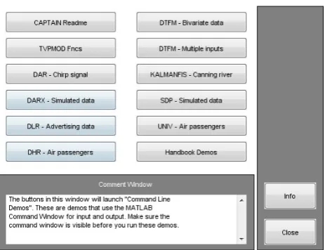
1.5 Starting the Demos
Once installed, typing captdemo in the MATLAB Command Window starts a simple graphical user interface for access to the Command Line demos. If this does not work, check that you have correctly added the toolbox locations to your MATLAB path. After typing captdemo (but before starting one of the demos) you can check the Command Window for a list of which modules have been added i.e.
>> captdemo
Checking MATLAB path... RIVSID installed TVPMOD installed TDCONT installed
Or, to open the Command Line demos for each module directly,
>> rivdemo >> tvpdemo >> tdcdemo
In each case, a simple graphical user interface provides access to the Command Line demos (e.g. Fig. 1.1). The latter utilise the Command Window for input and output, as well as generating graphs in a separate Figure Window, so make sure both of these are visible. Experience suggests that one of the most effective ways to get started with CAPTAIN is to examine each Command Line demo in turn and then to adapt them for each new data set of interest. Demo scripts can be opened in the MATLAB editor.
To obtain a full list of user functions for each module, type help rivsid, help tdcont or
help tvpmod in the Command Window, replacing rivsid, tdcont or tvpmod if necessary with the actual name of the folder (directory) chosen when you first installed the toolbox. To illustrate, the first few lines of the function list for TVPMOD are shown below.
>> help tvpmod Captain Toolbox
Time Variable Parameter Models
Unobserved Components Models.
dhr - Dynamic Harmonic Regression analysis. dhropt - DHR hyper-parameter estimation.
irwsm - Integrated Random Walk smoothing and decimation. irwsm - Integrated Random Walk smoothing and decimation. irwsmopt - IRWSM hyper-parameter estimation.
univ - Trend with Auto-Regression component. univopt - Trend with AR hyper-parameter estimation.
Time Variable and State Dependent Parameter Models.
dar - Dynamic Auto-Regression and time frequency analysis. daropt - DAR hyper-parameter estimation.
Figure 1.1 Demos for the TVPMOD module obtained by typing tvpdemo at the MATLAB Command Line.
Each function includes help information obtained in the usual manner e.g. help irwsm. Default input arguments are shown in parenthesis while (*) implies no default (hence a user input argument is always required for this variable). Some functions include more information, readable using e.g. type irwsm or edit irwsm (see Chapter 3 for details).
1.6 Caveat
CAPTAIN is a MATLAB compatible toolbox for non-stationary time series analysis and forecasting. Based around a powerful state space framework, CAPTAIN extends MATLAB to allow, in the most general case, for the identification of Unobserved Components (UC) models. Here, the time series is assumed to be composed of an additive or multiplicative combination of different components that have defined statistical characteristics but which cannot be observed directly. With Maximum Likelihood estimation of most models and the inclusion of several popular model forms, such as the Basic Structural Model of Harvey (1989) and the Dynamic Linear Model of West and Harrison (1989), together with a standard set of data pre-processing, system identification and model validation tools, CAPTAIN is a wide-ranging package for signal processing and general time series analysis.
Uniquely, however, CAPTAIN focuses on Time Variable Parameter (TVP) models, where the stochastic evolution of each parameter is assumed to be described by a generalised random walk process (Jakeman and Young, 1981). In this regard, the state space formulation utilised is particularly well suited to estimation based on optimal recursive estimation, in which the time variable parameters are estimated sequentially whilst working through the data in temporal order. In the off-line situation, where all the time series data are available for analysis, this Kalman filtering operation (Kalman, 1960) is accompanied by optimal recursive smoothing. Here the estimates obtained from the forward pass filtering algorithm are updated sequentially whilst working through the data in reverse temporal order using a backwards-recursive Fixed Interval Smoothing (FIS) algorithm (Bryson and Ho, 1969).
In this manner, CAPTAIN provides novel tools for TVP analysis, allowing for the optimal estimation of dynamic regression models, including linear regression, auto-regression (Young, 1998b) and harmonic regression (Young et al., 1999). Furthermore, a closely related algorithm for state dependent parameter estimation provides for the non-parametric identification and forecasting of a very wide class of nonlinear systems, including chaotic systems. The identification stage in this process again exploits the recursive FIS algorithms, combined with special data re-ordering and ‘back-fitting’ procedures, to obtain estimates of any state dependent parameter variations (Young, 2000).
Of course, in many cases, specifying time invariant parameters for the model yields the equivalent, conventional, stationary model. In this regard, one model that has received special treatment in the toolbox is the multiple-input, single-output Transfer Function (TF)
CHAPTER 2
model. CAPTAIN includes functions for robust unbiased identification and estimation of both discrete- time (Young, 1984, 1985) and continuous- time (Young, 2002) TF models. One advantage of the TF model is its simplicity and ability to characterise the dominant modal behaviour of a dynamic system. This makes such a model an ideal basis for control system design.
In the latter regard, the toolbox includes a set of functions for True Digital Control (TDC), based on the Proportional-Integral-Plus (PIP) control system design methodology (Young et al., 1987; Taylor et al. 2000, 2013). The underlying philosophy of the approach is that the entire design procedure, from the identification and estimation of a suitable model through to the practical implementation of the final control algorithm, is carried out in discrete time. This differs from many conventional digital controllers, where an inherently continuous time algorithm is digitised for implementation purposes. Indeed, CAPTAIN has been successfully utilised for the design of PIP control systems for many years (e.g. Taylor et al., 2004, 2013; Taylor and Shaban, 2006).
Some of the estimation algorithms considered here were developed originally in the 1960/1970/1980’s for the CAPTAIN and microCAPTAIN time series analysis and forecasting packages (MS-DOS based). The associated optimisation algorithms were developed in the 1980/1990’s and were used in the latest version of microCAPTAIN (Young and Benner, 1991). However, the MATLAB implementation is much more flexible than microCAPTAIN and includes the latest innovations and improvements to the algorithms. Note that the present text refers exclusively to this CAPTAIN Toolbox for MATLAB(Taylor et al., 2007).
2.1 Modelling Philosophy
As we look around us, we perceive complexity in all directions: environmental, biological and ecological systems, socio-economic systems, and some of the more complex engineering systems – they all appear to be complicated assemblages of interacting processes, many of which are inherently nonlinear dynamic systems, often with considerable uncertainty about both their nature and their interconnections. It is not too surprising, therefore, that the mathematical models of such systems, as constructed by scientists, social scientists and engineers, are often similarly complex.
What is perhaps surprising, however, is the apparently widespread belief that such systems can be described very well, if not exactly, by deterministic mathematical equations, with little or no quantification of the associated uncertainty. Such deterministic reductionism leads inexorably to large, nonlinear simulation models which reflect the popular view that complex systems must be described by similarly complex models.
statistical analysis required for the identification and estimation of such models. Furthermore, it stresses the importance of explicitly acknowledging the basic uncertainty that is essential to any characterisation of physical, chemical, biological and socio-economic processes.
Previous publications map the evolution of the DBM philosophy and its methodological underpinning. Such publications utilise the approach for the analysis of numerous natural and man-made systems. An incomplete list includes: Beck and Young (1975); Jarvis et al. (1999); Parkinson and Young (1998); Price et al. (1999, 2000, 2001); Shackley et al. (1998); Tych et al. (1999); Ye et al. (1998); Young (1978, 1981; 1983, 1984; 1985; 1993a, 1993b; 1994; 1998a, 1998b, 1999a, 1999b, 2000, 2001a, 2001b, 2002); Young and Beven (1994); Young and Lees (1993); Young and Minchin (1991); Young and Pedregal (1996; 1997; 1998, 1999a, 1999b); Young et al. (1996, 1997, 1999, 2000).
Naturally, these publications introduce a wide range of modelling tools, encompassing various model structures and identification algorithms. However, they can be broadly categorised into the four closely related and overlapping themes below.
1. Many of the tools that underpin the DBM modelling philosophy can be unified in terms of the discrete-time UC model. Here, the components may include a trend or low frequency component, a seasonal component (e.g. annual seasonality), additional sustained cyclical or quasi-cyclical components, stochastic perturbations, a component to capture the influence of exogenous input signals and so on. CAPTAIN allows for a wide range of such components.
2. Nonstationary and nonlinear signal processing based on the identification and estimation of stochastic models with time varying parameters. In this case, the term ‘nonstationarity’ is assumed to mean that the statistical properties of the signal, as defined by the parameters in an associated stochastic model, are changing over time at a rate which is ‘slow’ in relation to the rates of change of the stochastic state variables in the system under study. Although such nonstationary systems exhibit nonlinear behaviour, this can often be approximated well by TVP (or piece-wise linear) models, the parameters of which are recursively estimated.
3. Further to item 2. above, if the changes in the parameters are functions of the state or input variables (i.e. they actually constitute stochastic state variables), then the system is truly nonlinear and likely to exhibit severe nonlinear behaviour. Normally, this cannot be approximated in a simple TVP manner; in which case, recourse must be made to alternative, and more powerful in this context State Dependent Parameter (SDP) modelling methods.
where the latter is utilised in the present text) or continuous-time TF models based on the Laplace Transform s-operator are identified and estimated.
In recent versions of CAPTAIN, items 1–3 are addressed by TVPMOD, while item 4 is implemented in RIVSID. Finally, the independently developed TDCONT module uses discrete-time multivariable TF models obtained from RIVSID for control system design.
2.2 MATLAB
MATLAB is a high performance language published by The MathWorks, Inc., integrating computation, visualisation and programming in a single environment (MathWorks, 2017). CAPTAIN is a collection of MATLAB functions for the estimation of UC, TVP, SDP and TF models, and for PIP control system design. By also including a number of additional functions for data pre-processing, system identification and model validation, CAPTAIN provides a powerful all round package for the analysis of complex stochastic systems (Taylor et al. 2007). The following sections introduce the three main areas of functionality.
2.3 TVPMOD: Time Variable Parameter MODels
Unobserved Components models: CAPTAIN includes a range of UC models, a number of which are unique to this toolbox. In particular, the Dynamic Harmonic Regression (DHR) model, estimated using the function dhr, is very useful for signal extraction and forecasting of periodic or quasi-periodic series. This function provides smoothed estimates of the series, as well as all its components (trend, fundamental frequency and harmonic components), together with the estimated changing amplitude and phase of the latter. Typical applications are for the analysis of periodic environmental and economic time-series; restoration of noisy signals with gaps or other aberrations; and the evaluation of temporal changes in environmental data etc. Furthermore, the same function allows for the estimation of the well-known Basic Structural Models (BSM) of Harvey (1989).
It should be pointed out that, while it is sometimes convenient to categorise the functionality of the toolbox, there is considerable overlap between the methodological areas chosen. For example, the DHR model is a particular case of the general stochastic TVP model discussed in the following subsection. In this regard, the hyper-parameters of the model, which define the statistical properties of the time variable parameters, need to be estimated in some manner. CAPTAIN provides three approaches, all through the function dhropt, namely: Maximum Likelihood (ML) based on prediction error decomposition; minimisation of the multiple-steps-ahead forecasting errors; and a special frequency domain optimisation, based on fitting the model pseudo-spectrum to the logarithm of the Auto-Regression (AR) spectrum.
An alternative to dhr/dhropt is provided by the pair univ/univopt, which allow for the estimation of various additional UC model forms. Here, the trend is extracted from the time series and a peturbational component about the trend is modelled as a pure AR component. Although they may also be utilised for modelling seasonal series,
using either standard statistical methods or a sequential spectral decomposition approach that has been developed for the toolbox in order to avoid identifiably problems.
Time Variable Parameter models: the class of TVP, or ‘dynamic’, regression models, includes: Dynamic Linear Regression (DLR), Dynamic Harmonic Regression (DHR), Dynamic Auto-Regression (DAR), Dynamic Auto-Regression with eXogenous variables (DARX) and the closely related Dynamic Transfer Function (DTF) model. It should be noted that the term ‘dynamic’, which is used to differentiate time variable parameter regression models from their standard constant parameter relatives, is somewhat misleading, since not all of these models are inherently dynamic in a systems sense. However, it is a common term in certain areas of statistics (see e.g. West and Harrison, 1989 and the references therein) and is retained for this reason.
CAPTAIN provides functions that allow for the optimal estimation of all these dynamic regression models. In each case, Fixed Interval Smoothing (FIS) estimates of the TVPs are obtained, under the assumption that the parameters vary as one of a family of generalised random walks namely: Random Walk (RW); Integrated Random Walk (IRW); Smoothed Random Walk (SRW); and Local Linear Trend (LLT). The associated filtering and FIS algorithms are accessible via shells, namely the functions dlr, dhr, dar, darx and dtfm. Since the regressors are freely defined by the user, the most flexible toolbox function for TVP analysis is dlr, which can include all the remaining models as special cases. The other functions all restrict the model to the most commonly used forms. For example, dhr
automatically constrains the regressors to model harmonic components. As one of the key tools for estimating UC models, it has already been discussed above.
At this juncture, it is worth pointing out that CAPTAIN includes the functions mar and
arspec for Auto-Regression (AR) model and spectrum estimation. However, in the context of dynamic regression, dar and darsp are instead useful for evaluating changing signal spectra and time-frequency analysis based on DAR models, since they provide the AR spectrum at each point in time based on the locally optimum time variable AR parameters.
Further to this, darx is an extension of the DAR model to include measured eXogeneous or input time series that are thought to affect the output, while dtfm augments the model in order to allow for coloured noise in the output signal. The latter function employs instrumental variables in the solution to ensure that the parameter estimates are unbiased. In this manner, the functions darx and dtfm are truly dynamic in a systems sense and form a link between the dynamic regression analysis considered here and the dedicated TF modelling component of the toolbox discussed in the next section.
In the case of dlr, dar, darx and dtfm, the Noise Variance Ratio (NVR) and other hyper-parameters, which define the statistical properties of the TVP’s, are optimised via ML based on prediction error decomposition. The relevant toolbox functions are dlropt,
State Dependent Parameter models: the approach to TVP estimation discussed above works very well in situations where the parameters are slowly varying when compared to the observed temporal variation in the measured system inputs and outputs. Although such models are nonlinear systems, since the same inputs, injected at different times, will elicit quite different output responses, the resultant nonlinearity is fairly mild. It is only when the parameters are varying at a rate commensurate with that of the system variables themselves that the model behaves in a heavily nonlinear or even chaotic manner. For such cases, CAPTAIN includes a novel algorithm for state dependent parameter estimation, sdp, allowing for the non-parametric identification and forecasting of a very wide class of nonlinear systems.
Specifying time invariant parameters for the above TVP models usually yields the equivalent stationary time series model. In this manner, many of the functions above may be utilised to estimate either the well-known conventional model or the more sophisticated TVP version, depending on the input arguments chosen.
System identification is inherent to the modelling approach utilised by most of the functions already discussed. Identification tools not yet mentioned include, for example,
acf to determine the sample and partial autocorrelation function; ccf for the sample cross-correlation; period to estimate the periodogram; and statist for some sample descriptive statistics. Furthermore, del generates a matrix of delayed variables, fcast may be employed to prepare data for forecasting and interpolation, and irwsm is used for smoothing, decimation or for fitting a simple trend to a time series. These examples complement various other included auxiliary functions (see toolbox help for details).
2.4 RIVSID: Refined Instrumental Variable System Identification
Multi-Input Transfer Function models: although there are numerous algorithms for estimating TF models, the primary technique employed in CAPTAIN, is the least squares- based instrumental variable approach. Here, an adaptive auxiliary model is introduced into the solution in order to avoid parameter bias and to optimally filter the data, so making the estimation more statistically efficient. In particular, CAPTAIN provides the recursive and en-block RIV algorithms, as well as more conventional least squares based approaches, primarily through the functions rivbj (for discrete-time systems) and rivcbj (continuous-time). Both these functions return the modelling results in the form of a special matrix from which the various parameters and standard errors may be extracted using getparbj. Such parameters are subsequently be utilised for simulation and forecasting through conventional MATLAB commands like filter, or by using SIMULINK® (MathWorks, 2017).
Since 2007, CAPTAIN has allowed for the estimation of TF models with an auto-regressive, moving average (ARMA) noise component, i.e. full Box-Jenkins (BJ) models. The functions for TF modelling listed above allow for such BJ models (or simpler models as special cases using the input arguments). However, older CAPTAIN algorithms that are limited to an AR noise model are still included for backwards compatibility (with long time users of the toolbox) and sometimes as a back-up option. These functions are called
riv/rivid, rivc/rivcid and getpar.
Finally, the toolbox includes various data preparation and auxiliary functions, including, for example, prepz to prepare data for input-output modelling and prbs for generating a Pseudo Random Binary Signal (PRBS), among others.
2.5 TDCONT: True Digital CONTrol (TDC)
True Digital Control: following the identification of a suitable discrete-time time TF model, PIP control systems are determined using either the pip or pipopt functions, for pole assignment or linear quadratic optimal design respectively. These functions are for the single input, single output (SISO) case, while mpipdc and mpiplq are used for multivariable PIP control design (for which mtf2mfd is used to convert a multivariable TF into the required Matrix Fraction Description). Furthermore, dlrqrf provides direct access to the iterative linear quadratic regulator solution for either the SISO or multivariable cases; while tdclib is the Simulink® library for various PIP control structures, including the
conventional feedback form and an alternative forward path approach.
The PIP approach is based on the definition of Non-Minimal State Space (NMSS) models, using either nmss (SISO) or mfd2nmss (multivariable), so that full state variable feedback control can be implemented directly from the measured input and output signals of the controlled process. The PIP controller can be interpreted as a logical extension of Proportional-Integral-Derivative (PID) control, with additional dynamic feedback and input compensators introduced automatically, when the process has second order or higher dynamics or pure time delays greater than one sampling interval.
The following examples aim to provide a brief illustration of toolbox functionality for users already familiar with the methodology, or at least to introduce some of the ideas to the open minded reader who is not. In this regard, it should be pointed out that formal stochastic descriptions of the models are omitted from this Getting Started Guide.
Installation instructions and conditions of use are given in Chapter 1. It is assumed that all three modules, RIVSID, TDCONT and TVPMOD are installed. Since CAPTAIN is largely a command line toolbox, it is also assumed that the reader is already familiar with basic MATLAB usage, such as loading data, plotting graphs and writing simple M-files. Introductory guides include Etter (1993) and Biran and Breiner (1995). Hence, for brevity, the straightforward MATLAB code to label the plots and set the axis limits etc. is not necessarily shown in the examples below.
Example 3.1 IRW smoothing of the airline passenger series
To plot the well-known airline passenger series (e.g. Box and Jenkins, 1970), enter the following text at the MATLAB Command Window prompt,
>> load air.dat >> plot(air)
>> title('thousands of passengers per month (1949-1960)')
These data are included in the TVPMOD module for demonstration purposes, in a standard text file. If an error occurs, then check that you have correctly added the toolbox location to your MATLAB path.
We will smooth these data using irwsm. In general, the brief calling syntax for each function in CAPTAIN is obtained by entering its name without any input arguments:
>> irwsm
irwsm Integrated Random Walk smoothing and decimation
[ys,deriv,fitse,trse,derivse,y0,PkN,ers,ykk1,er]=...
irwsm(y,TVP,nvr,Int,dt,delt)
CHAPTER 3
More information is provided using the standard help command, as illustrated below. In this case, each input argument is described in turn, followed by the output arguments and any other information.
>> help irwsm
irwsm Integrated Random Walk smoothing and decimation
[ys,deriv,fitse,trse,derivse,y0,PkN,ers,ykk1,er]=...
irwsm(y,TVP,nvr,Int,dt,delt)
y: Time series (*)
TVP: Model type (RW=0, IRW=1, DIRW=2) (1) nvr: NVR hyper-parameter (1605*(1/(2*dt))^4) Int: Vector of variance intervention points (0) dt: decimation rate (1)
with dt>1 only the following returned arguments are decimated: ys, deriv, fitse, trse, derivse, y0 delt: sampling rate (1)
ys: Decimated (or simply smoothed if dt=1) series deriv: Derivatives
fitse: Standard error of model fit (including observation noise) trse: Trend (state) standard error
derivse: standard error of the remaining states (trend derivs.) y0: Interpolated data
...
The on-line help messages in CAPTAIN are deliberately concise. This is so that an experienced user can find information quickly. However, many functions include supplementary information, readable using:
>> type irwsm
The supplementary information can also be examined by opening the m-file in an editor and scrolling down to find it:
>> edit irwsm
In the help information, default values for any optional inputs are given in brackets, whilst any necessary inputs, such as the data vector y above, are listed with an asterix (*). In this case, the default TVP = 1 implies the following model based on an IRW model plus noise,
t t t T e
y (3.1)
t t t
t T T
T 2 1 2 (3.2)
respectively. Here, Tt is effectively a time variable parameter, whose stochastic evolution in the form of an IRW is described by equation (3.2). Finally, t and et are independent zero mean white noise sequences with variance q2 and 2, representing the system disturbances and measurement noise respectively. The present Getting Started Guide omits a full explanation of this model and the state space form actually used for estimation: see additional toolbox documentation for details.
Empty variables [ ] may be used to indicate default values when a mixture of defaults and user specified arguments are required. For example, a smoothed trend is fitted to the airline passenger series as follows,
>> load air.dat
>> t = irwsm(air, [], 0.0001); % equivalent to t = irwsm(air, 1, 0.0001) >> plot([air t])
[image:18.595.174.430.364.580.2]The plot compares the smoothed and original series, as illustrated in Fig. 3.1. Note that the 3rd input argument to irwsm specifies the associated Noise Variance Ratio (NVR) hyper-parameter. Defined here as q2 2 0.0001, this variable is closely related to the bandwidth of the filter. Try using values of e.g. 0.1 and 0 for this fourth input argument.
Figure 3.1 Thousands of airline passengers per month (1949-1960) and IRW trend.
Example 3.2 Interpolation of advertising data using DLR
0 10 20 30 40 50 60 70 80 90 0 0.1 0.2 0.3 0.4 R es po ns e
0 10 20 30 40 50 60 70 80 90
0 200 400 600 800 E xp en di tu re
[image:19.595.115.487.91.390.2]Time (sample number)
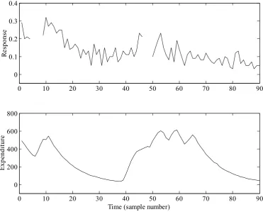
Figure 3.2 Scaled advertising data plotted against an arbitrary fixed sampling rate.
Top: response to advertising. Bottom: expenditure on advertising.
For the purposes of the example, these confidential data have been scaled in an arbitrary manner, so no units are given in the plots. The output response data are in the range 0-1, where a larger number implies a more successful response to the advertising. It is clear that the response data contain missing values, represented in MATLAB by special Not-a-Number or nan values and forming gaps in the top plot of Figure 3.2. The filtering and smoothing algorithms implemented in CAPTAIN automatically account for these.
For a preliminary analysis of these data, we will utilise the following model,
90 ..., , 2 , 1
T bu e t
yt t t t t (3.3)
where yt is the response and ut is the expenditure, while Tt and bt are the time variable
parameters. Finally, et is a serially uncorrelated and normally distributed Gaussian sequence with zero mean value and variance 2. Note that a full description of the general
DLR methodology and state space model is omitted from this Getting Started Guide.
For constant parameters Tt T and bt b, equation (3.3) takes the form of a conventional regression model based on the equation of a straight line. However, here we utilise dlropt
>> load adv.dat
>> u = adv(:, 1); % expenditure >> y = adv(:, 2); % response
>> z = [ones(size(u)) u]; % regressors >> nvr = dlropt(y, z)
nvr = 0.0078 0.0000
While dlropt is running, a window will briefly appear on screen indicating the optimisation algorithm being utilised, together with an update of the Log-Likelihood.
It should be pointed out that default values for the toolbox have been carefully chosen, in order to be as widely applicable as possible. In the present case, the default initial conditions and optimisation settings converge to a solution without any problem, hence only the first two input arguments are required.
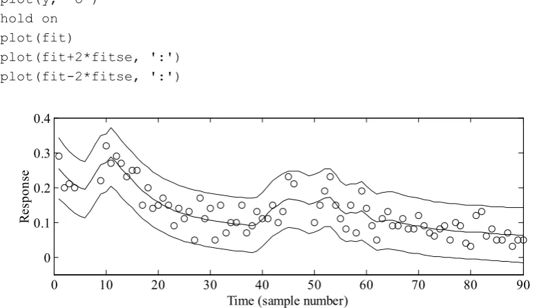
From this analysis, it appears that the Tt level or trend parameter varies significantly over time (NVR = 0.0078), while the bt slope parameter is relatively time invariant and has a NVR value close to zero. To determine the fit and parameters,
>> [fit, fitse, par] = dlr(y, z, [], nvr);
By default, dlr assumes NVR’s of zero, so the 4th input argument above is necessary to specify the previously optimised values. The 3rd input argument selects the model type: in this case, empty brackets imply the default random walk model. Examination of the parameters, returned as the first and second columns of par, show how these evolve gradually over time (not plotted here). The model fit and associated standard errors are shown in Figure 3.3, which is obtained using the code below,
>> plot(y, 'o') >> hold on >> plot(fit)
>> plot(fit+2*fitse, ':') >> plot(fit-2*fitse, ':')
0 10 20 30 40 50 60 70 80 90
0 0.1 0.2 0.3 0.4
R
es
po
ns
e
[image:20.595.103.492.505.728.2]Time (sample number)
Figure 3.3 Scaled response to advertising plotted against an arbitrary fixed sampling rate.
It is clear from Figure 3.3 that the data all lie within the standard error bounds. Note also that no user intervention was required to interpolate over the missing response data: both
fit and par apply over the entire time series. Refer to the on-line help for a full list of optimisation settings and output arguments. For example, dlr can return the interpolated output y0, consisting of the original series with any missing data replaced by the model fit.
Example 3.3 Transfer Function model estimation using RIV
Many control systems, both classical and modern, are analysed by means of TF models. Indeed, CAPTAIN has been successfully utilised for the design of control systems for many years, particularly with regards to the development of PIP control methods (see Taylor et al. 2013 for numerous examples). One practical application is concerned with forced ventilation in animal houses (Taylor et al., 2004). Here, uncontrolled data are first collected in order to identify the dominant dynamics of the fan.
For a particular test installation at the Katholieke Universiteit Leuven, the SRIV algorithm, combined with the RT2 and YIC identification criteria, reveal that a first order model with 6 seconds time delay provides the best estimated model and most optimum fit to the data across a wide range of operating conditions. In a typical experiment, based on a 2 second sampling rate, the SRIV algorithm yields the following difference equation,
3 1 79.8
438 .
0
t t
t y u
y (3.4)
where yt is the airflow rate (m3/h) and
t
u is the applied voltage to the fan expressed as a percentage. Equation (3.4) shows that the output variable yt, is a simple linear function of its value at the previous sample and the delayed input variable. Equation (3.4) may alternatively be represented in terms of the backward shift operator L, i.e. Ljyt yt j
, by the following discrete-time TF model,
t t u L L y 438 . 0 1 8 . 79 3 (3.5)
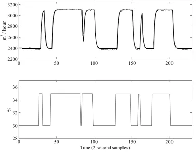
The response of the model (3.5) closely follows the noisy measured data, as illustrated by Figure 3.4. These data are included with CAPTAIN for demonstration purposes and the associated MATLABcommands for estimating the model are shown below.
>> load vent.dat
>> [z, m] = prepz(vent, [], 25);
>> [th, stats, e] = riv(z, [1 1 3 0]); >> [at, bt] = getpar(th)
at =
1.0000 -0.4381 bt =
0 0 0 79.7835 >> rt2 = stats(3)
>> subplot(211); plot([z(:, 1) z(:, 1)-e]+m(1)) >> subplot(212); plot(z(:, 2)+m(2))
Here, the experimental data are organised into matrix form, with the first column of vent
consisting of the output variable yt, and the second the input variable ut. The function
prepz is utilised to prepare the data for modelling. In particular, the 3rd input argument subtracts the mean of the first 25 samples from the data in order to remove the baseline from the series. Such data pre-processing sometimes yields better results in the context of TF model estimation.
The TF is estimated using riv, where the second input argument defines the model structure: in this case, 1 denominator parameter, 1 numerator parameter, 3 samples time delay and no model required for the noise. Refer to the function help information for a full description of the TF modelling tools and the syntax required. In particular, note that MISO and continuous-time models are also possible, while additional functions allow for the identification of the most appropriate model structure.
The first output argument, th, is a matrix containing information about the TF model structure, the estimated parameters and their estimated accuracy. In this case, getpar is utilised to extract the required parameter estimates for later control system design. Note that these parameter vectors include the leading unity of the TF denominator, and that the time delays are represented as zero valued elements in the numerator.
0 50 100 150 200
2200 2400 2600 2800 3000 3200
m
3 /
ho
ur
0 50 100 150 200
28 30 32 34 36
Time (2 second samples)
[image:22.595.105.490.423.722.2]%
Figure 3.4 Top: ventilation rate (m3/h) and response of the identified TF model (thick trace)
The second output argument, stats, lists nine statistical diagnostics associated with the model, including RT2 0.9873, implying that the model describes nearly 99% of the variation in the data. Finally, the modelling errors are returned as the variable e and are used in the code above to compare the TF response with the original data, as shown in Figure 3.4. In this graph, the baseline is returned to the series. The built-in MATLAB function filter may also be employed to simulate the TF response using these parameter vectors. This is useful for simulation and (if estimates of the future input variable are available) forecasting purposes.
Example 3.4 PIP Control Design and Simulation
Consider again the ventilation system introduced by Example 3.3 and the associated TF model (3.4) or (3.5). The digital control algorithms developed below require that the model has at least one sample pure time delay and that the first element of the denominator polynomial is unity. For these reasons, the model will be defined in MATLAB as follows:
>> a=-0.4381 % denominator polynomial with leading unity removed >> b=[0 0 79.7835] % numerator with one sample time delay removed
Help messages for functions in the TDCONT module often refer to this ‘truncated form’ of the TF polynomials. For the present example, the NMSS model is defined by the non-minimal state vector, [ 1 2 ]T
t y u ut t t zt
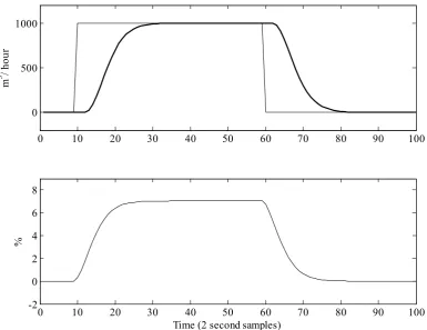
x , in which zt is the integral-of-error between the reference or command input rt and the sampled output i.e. zt zt1 rt yt. The reader is directed to one of the many articles on PIP control for details of the design approach; see e.g. Taylor et al. (2000, 2004, 2013) and the references therein. The commands below specify closed-loop poles for the ventilation system and plot the time response. For the purpose of this example, the poles have been arbitrarily chosen within the unit circle on the complex z-plane as follows: 0.5, 0.60.1i and 0.7.
>> k = pip(a, b, [0.5 0.6+0.1i 0.6-0.1i 0.7]); % control gains >> [acl, bcl, bclu] = pipcl(a, b, k); % closed-loop TF >> r = zeros(100, 1); r(10:59) = ones(50, 1)+1000; % command input >> y = filter(bcl, acl, r); subplot(211); plot([y r]) % output variable >> u = filter(bclu, acl, r); subplot(212); plot(u) % input variable
The output argument of the pole assignment algorithm, pip, is the control gain vector. Linear quadratic design is achieved using pipopt instead, for which the input arguments specify weights on the integral-of-error state, input states and output states. In the code above, pipcl determines the closed-loop TF i.e. the relationships between rt and the input or output variables. The MATLABfunction filter uses these to evaluate the time response, as illustrated in Figure 3.5. To confirm that the closed-loop poles are those expected:
>> roots(acl) ans =
0 10 20 30 40 50 60 70 80 90 100 0
500 1000
m
3 / h
ou
r
0 10 20 30 40 50 60 70 80 90 100
-2 0 2 4 6 8
%
Time (2 second samples)
[image:24.595.106.492.69.366.2]
Figure 3.5 Top: ventilation rate command input and simulated closed-loop response (thick trace).
Bottom: simulated applied voltage expressed as a percentage.
The function pipgains returns the control polynomials if desired:
>> [fpip, gpip, kpip]=pipgains(a, b, k) fpip =
0.00024 gpip =
1.0000 -0.9619 0.3386 kpip =
0.00032
In this case, the proportional gain f00.00024, the denominator of the input filter 2
( ) 1 0.9619 0.3386
G L L L and the integral gain kI 0.00032. This brief example omits many details, including the block diagram form of the PIP controller. The included demos in the toolbox provide MATLAB code for reproducing almost all of the examples in the book by Taylor et al (2013). The book provides a tutorial introduction to multivariable state space control system design with numerous worked examples, block diagrams, and guidance on the practical implementation of the control systems developed.
3.4 Concluding Remarks
Beck, M.B. and Young, P.C. (1975) A Dynamic Model for DO-BOD Relationships in a Non-Tidal Stream, Water Research, 9, 769-776
Biran, A. and Breiner, M. (1995), MATLAB for Engineers, Addison Wesley.
Box, G.E.P. and Jenkins, G.M. (1970), Time Series Analysis: Forecasting and Control, revised edn, San Francisco: Holden-Day, 1976.
Bryson, A.E. and Ho, Y.C. (1969) Applied Optimal Control, Optimization, Estimation and Control, Waltham: Blaisdell Publishing Company.
Etter, D.M. (1993), Engineering problem solving with MATLAB, Prentice-Hall.
Harvey, A.C. (1989), Forecasting Structural Time Series Models and the Kalman Filter, Cambridge: Cambridge University Press.
Jakeman, A.J. and Young, P.C. (1981) Recursive filtering and the inversion of ill-posed causal problems, Utilitas Math, 25, 351-376.
Jarvis, A.J., Young, P.C., Taylor, C.J. and Davies, W.J. (1999) An analysis of the dynamic response of stomatal conductance to a reduction in humidity over leaves of cedrella odorata, Plant, Cell and Environment, 22, 913-924.
Kalman, R.E. (1960), A new approach to linear filtering and prediction problems, ASME Transactions Journal Basic Engineering, 83-D , 95-108.
Mathworks, The, (2017) Matlab (www.mathworks.com).
Parkinson, S. and Young, P.C. (1998) Uncertainty and sensitivity in global carbon cycle modelling, Climate Research, 9, 157-174.
Pedregal, D.J., Taylor, C.J. and Young, P.C. (2007) System Identification, Time Series Analysis and Forecasting: The Captain Toolbox, Lancaster University.
Price, L., Young, P., Berckmans, D., Janssens, K. and Taylor, J. (1999) Data-Based Mechanistic Modelling (DBM) and Control of Mass and Energy transfer in agricultural buildings, Annual Reviews in Control, 23, 71-82.
Price, L.E., Goodwill, P., Young, P.C. and Rowan, J.S. (2000) A data-based mechanistic modelling (DBM) approach to understanding dynamic sediment transmission through Wyresdale Park Reservoir, Lancashire, UK, Hydrological Processes, 14, 1, 63-78. Price, L.E., Bacon, M.A., Young, P.C. and Davies, W.J. (2001) High-resolution analysis of
tomato leaf elongation: the application of novel time-series analysis techniques, Journal of Experimental Botany, 52, 362, 1925-1932.
Shackley, S., Young, P.C., Parkinson, S. and Wynne, B. (1998) Uncertainty, complexity and concepts of good science in climate change modelling: are GCMs the best tools? Climate Change, 38, 159-205.
Taylor, C.J. and Shaban, E.M. (2006) Multivariable Proportional-Integral-Plus (PIP) control of the ALSTOM nonlinear gasifier simulation, IEE Proceedings Control Theory and Applications, 153, 3, 277-285.
Taylor, C.J., Chotai, A. and Young P.C. (2000) State space control system design based on non-minimal state-variable feedback: Further generalisation and unification results, International Journal of Control, 73, 1329-1345.
Taylor, C.J., Leigh, P., Price, L., Young, P.C., Berckmans, D., Janssens, K., Vranken, E. and Gevers, R. (2004) Proportional-Integral-Plus (PIP) control of ventilation rate in agricultural buildings, Control Engineering Practice, 12, 2, 225-233.
Taylor, C.J., Pedregal, D.J., Young, P.C. and Tych, W. (2007) Environmental Time Series Analysis and Forecasting with the CAPTAIN Toolbox, Environmental Modelling and Software, 22, 797-814.
Taylor, C.J., Young, P.C. and Chotai, A. (2013) True Digital Control: Statistical Modelling and Non–Minimal State Space Design, John Wiley & Sons Ltd.
Tych, W., Young, P.C., Pedregal, D. and Davies, J. (1999) A software package for multi-rate unobserved component forecasting of telephone call demand. International Journal of Forecasting.
West, M. and Harrison, J. (1989) Bayesian Forecasting and Dynamic Models, New York: Springer-Verlag.
Young, P.C. (1978) A general theory of modeling for badly defined dynamic systems, in G.C. Vansteenkiste (ed.), Modeling, Identification and Control in Environmental Systems, North Holland: Amsterdam, 103-135.
Young, P.C. (1981) Parameter estimation for continuous-time models - a survey, Automatica, 17, 23-39.
Young, P.C. (1983) The validity and credibility of models for badly defined systems, in M.B. Beck and G. Van Straten (eds.), Uncertainty and Forecasting of Water Quality, Springer Verlag: Berlin, 69-100.
Young, P.C. (1984) Recursive Estimation and Time-Series Analysis, Berlin: Springer-Verlag.
Young, P.C. (1985) The instrumental variable method: a practical approach to identification and system parameter estimation. In: Barker, H. A. and Young, P.C. (Eds.), Identification and System Parameter Estimation, Pergamon: Oxford, 1-15. Young, P.C. (1993a) Concise Encyclopedia of Environmental Systems, Oxford: Pergamon
Press.
Young, P.C. (1993b) Time variable and state dependent modelling of nonstationary and nonlinear time series. In: Subba Rao. T. (Ed.), Developments in time series analysis, Chapman and Hall: London, 374-413.
Young, P.C. (1994) Time-variable parameter and trend estimation in non-stationary economic time series, Journal of Forecasting, 13, 179-210.
Young, P.C., (1998b) Data-based mechanistic modelling of environmental, ecological, economic and engineering systems, Environmental Modelling and Software, 13, 105-122.
Young, P.C. (1999a) Nonstationary time series analysis and forecasting, Progress in Environmental Science, 1, 3-48.
Young, P.C. (1999b) Data-based mechanistic modelling, generalised sensitivity and dominant mode analysis, Computer Physics Communications, 117, 113-129.
Young, P.C. (2000) Stochastic, dynamic modelling and signal processing: time variable and state dependent parameter estimation. In: W. J. Fitzgerald et al. (Eds.) Nonlinear and nonstationary signal processing, Cambridge University Press: Cambridge, 74-114. Young, P.C. (2001a) The identification and estimation of nonlinear stochastic systems. In:
A.I. Mees (Ed.), Nonlinear Dynamics and Statistics, Birkhauser: Boston.
Young, P.C. (2001b) Comment on ‘A quasi-ARMAX approach to the modelling of nonlinear systems’ by J. Hu et al., International Journal of Control, 74, 1767-1771. Young, P.C. (2002) Optimal IV identification and estimation of continuous-time TF
models, International Federation of Automatic Control Triennial World Congress, Barcelona.
Young, P.C. and Benner, S. (1991) microCAPTAIN 2 User handbook, Centre for Research on Environmental Systems and Statistics, Lancaster University.
Young, P.C. and Beven, K.J. (1994) Data-based mechanistic modelling and the rainfall-flow nonlinearity’, Environmetrics, 5, 335-363.
Young, P.C. and Lees, M.J. (1993) The Active Mixing Volume (AMV): a new concept in modelling environmental systems, Chapter 1 in V. Barnett and K.F. Turkman (eds.), Statistics for the Environment. J. Wiley: Chichester, 3-44 .
Young, P.C. and Minchin, P. (1991) Environmetric time-series analysis: modelling natural systems from experimental time-series data, Int. J. Biol. Macromol., 13, 190-201. Young, P.C. and Pedregal, D.J. (1996) Recursive fixed interval smoothing and the
evaluation of LIDAR measurements: A comment on the paper by Holst et al. Environmetrics, 7, 417-427.
Young, P.C. and Pedregal, D.J. (1997) Data-Based Mechanistic Modelling, in C. Heij et al. (eds.), System Dynamics in Economic and Financial models, Chichester: J. Wiley. Young, P.C. and Pedregal, D.J. (1998) Data-based mechanistic modelling (of macro
economic systems). Chapter 6 in C. Heij et al (Eds.), System Dynamics in Economic and Financial Models, J. Wiley: Chichester and new York.
Young, P.C. and Pedregal, D.J. (1999a) Macro-economic relativity: government spending, private investment and unemployment in the USA 1948-1998, Structural Change and Economic Dynamics, 10, 359-380.
Young, P.C. and Pedregal, D.J. (1999b) Recursive and en bloc approaches to signal extraction. Journal of Applied Statistics, 26, 103-128.
Young, P., Parkinson, S. and Lees, M. (1996) Simplicity Out Of Complexity: Occam's Razor Revisited, Journal Of Applied Statistics, 23, 165-210.
Young, P.C., Jakeman, A.J. and Post, D.A. (1997) Recent advances in the data-based modelling and analysis of hydrological systems. Water Science and Technology, 36, 99-116.
Young, P.C. Pedregal D.J. and Tych, W. (1999) Dynamic Harmonic Regression, Journal of Forecasting, 18, 369-394.