Aerial Small Cells Using Coordinated
Multiple UAVs: An Energy Efficiency
Optimization Perspective
CHENGXIAO LIU 1, WEI FENG 1, (Senior Member, IEEE), JUE WANG 2, (Member, IEEE),
YUNFEI CHEN 3, (Senior Member, IEEE), AND NING GE 1, (Member, IEEE)
1Beijing National Research Center for Information Science and Technology, Tsinghua University, Beijing 100084, China 2Nantong Research Institute for Advanced Communication Technologies, Nantong University, Nantong 226019, China 3School of Engineering, University of Warwick, Coventry CV4 7AL, U.K.
Corresponding author: Wei Feng ([email protected])
This work was supported in part by the Beijing Natural Science Foundation under Grant L172041, in part by the National Natural Science Foundation of China under Grant 61771286, Grant 61701457, Grant 61771264, and Grant 91638205, and in part by the Beijing Innovation Center for Future Chip.
ABSTRACT Recently, unmanned aerial vehicle (UAV) communications have attracted great research interest. Due to the limited on-board energy, the optimization of energy efficiency (EE) is critical for UAV communications. In this paper, we propose an EE maximization scheme for UAV swarm-enabled small cell networks using large-scale channel state information at the transmitter (CSIT). The proposed scheme provides an agile coordination strategy for the UAVs in a swarm under energy constraints. We first formulate the EE maximization problem, where the objective function is defined as the ratio of the ergodic total data size to the total energy consumption. After that, an accurate approximation is derived to remove the intractable expectation operator in the objective function. As the newly formulated problem is non-convex, we decompose it into two subproblems to optimize the transmit power and the hovering time in an iterative way. Further by leveraging the max-min and linear optimization tools, both subproblems are efficiently solved. Simulation results demonstrate the superiority of our EE maximization scheme.
INDEX TERMS Coordinated power allocation, energy efficiency, small cell, time scheduling, unmanned aerial vehicle.
I. INTRODUCTION
Nowadays, unmanned aerial vehicle (UAV) communications have attracted great research interest [1], [2]. Deployed as mobile aerial base stations (BSs), the UAVs can adapt to the increasing demand for mobile terminals (MTs) in a vast coverage area, whereas the coverage area of conventional terrestrial BSs is usually limited [2], [3]. Therefore, UAV communications have been regarded as promising techniques for future networks [1]–[5].
In practice, the endurance of UAVs is an essential issue to be addressed in the design of UAV communi-cation networks [1], [2]. As most rotary-wing UAVs are small-sized and battery-powered [1], the on-board energy of UAVs, including the propulsion energy and the commu-nication energy, is extremely limited [2], [6]. Hence, the
The associate editor coordinating the review of this article and approving it for publication was Chi-Tsun Cheng.
optimization of energy efficiency (EE) is critical for UAV-enabled networks, where a number of related works have been conducted [7]–[12]. Zeng et al. optimized the EE of UAVs in [7], considering the energy consumption of UAV propulsion. Mozaffari et al.maximized the EE con-sidering the total uplink power constraint of the Internet of Things (IoT) devices in [8]. Liu et al.proposed a novel UAV control strategy in [9], which maximized the EE through deep reinforcement learning. Song et al. maximized the EE of multi-antenna UAV-enabled mobile relay in [10], which dis-cussed the trade-off between the throughput and propulsion energy consumption. Zhou et al.optimized the EE of UAVs for industrial internet in [11], which proposed a UAV control strategy in smart grid. Ghorbel et al.minimized the energy consumption of UAVs to optimize the EE in [12], which used the cognitive radio techniques.
proposed a scheme to cover a given area with the minimum number of UAVs. In [14], an energy-efficient multi-UAV cov-erage algorithm was proposed based on the game-theoretic framework. In [15], a UAV swarm path planning algorithm was proposed considering the propulsion energy consump-tion of UAVs. The authors of [16] optimized the trajectory of a UAV swarm to serve users in a network using the shortest time. In [17], a distributed UAV flocking model was proposed based on the positioning and communication techniques. In [18], a layered UAV swarm network structure was proposed using a low-latency routing algorithm. The authors of [19] optimized the spectrum efficiency and EE jointly through trajectory planning. In [20], the positioning of UAVs was optimized using deep Q-learning technique in dynamic UAV swarm networks. To further improve the per-formance of UAV swarm-enabled networks, aerial small cells were considered, where the UAVs work as small cells to pro-vide high-speed services in a coordinated manner [21]–[23]. In [21], a dynamic path planning algorithm was proposed for UAV-based aerial small cells. The authors of [22] pro-posed an energy-aware 3D deployment algorithm for UAV swarm-based aerial small cells. In [23], the coverage of mul-tiple UAVs was maximized in the presence of co-channel interference.
Due to the increasing service demand, the communi-cation energy consumption of UAVs becomes consider-able, which should be taken into account in the system design [15], [24], [25]. The authors of [15] considered the communication energy consumption in UAV path planning schemes to maximize the sum rate. In [24], the communica-tion energy was minimized by scheduling the hovering time of UAVs. In [25], we jointly optimized the communication energy and hovering time to maximize the total data size for UAV-aided IoT communications. However, the optimization of EE for UAV-swarm enabled small cell networks has not been addressed in any of the previous works.
In this paper, we address the EE maximization issue for UAV swarm-enabled small cell networks. Motivated by practical constraints, we assume only the slowly-varying large-scale channel state information (CSI) is available for optimization. In contrast, a simplified free-space path-loss channel model was assumed in most previous works [15], [16], [18], [24]. While adopting the simplified channel model can facilitate the mathematical analysis, it deviates from the realistic UAV channel conditions, which may cause severe performance degradation [25]. To char-acterize a realistic communication environment, a compos-ite channel model was considered in the design of UAV swarm-enabled small cell networks [25], [26]. This model considers both the line-of-sight (LOS) and non-line-of-sight (NLOS) channel elements, so that it is more practical than the simplified models. Concretely, this model includes both the large-scale channel fading, i.e. the position-related slowly-varying CSI, and the small-scale channel fading, i.e. the stochastic fast-varying CSI. It is worth noting that the small-scale CSI at the transmitter (CSIT) is in
general not available prior to the UAV flight due to its inherent unpredictability. However, the large-scale CSIT can be acquired [25], [27], thanks to the fact that both the pre-scheduled trajectory of UAVs and the locations of MTs can be known prior to the flight [15], [16]. The main contri-butions of this paper are summarized as follows.
• We formulate an EE maximization problem for UAV
swarm-enabled small cell networks with large-scale CSIT, where the objective is to maximize the ratio of the ergodic total data size to the total energy consumption. We propose an accurate approximation using a newly derived analytic function to remove the intractable expectation operator in the objective function to simplify the problem.
• We further decompose the simplified EE maximization problem into two subproblems. One subproblem is to find the optimal coordinated power allocation strategy, which is a nonlinear fractional optimization problem and known to be non-convex. An iterative algorithm is pro-posed to solve this subproblem. The other subproblem is to find the optimal hovering time scheduling strategy, which is a linear fractional optimization problem and can be efficiently solved after a series of reformulations.
• Based on the solutions to the two subproblems, i.e. the
power allocation strategy and the hovering time schedul-ing strategy, we propose an iterative algorithm to solve the original EE maximization problem with guaranteed convergence. Simulation results demonstrate the superi-ority of the proposed algorithm.
The rest of this paper is organized as follows. In Section II, we introduce the system model and the channel model, where the formulation of the proposed EE maximization problem is also introduced. The solution to the EE maximization prob-lem is given in Section III. Section IV presents the simulation results and discussions. Section V gives the conclusion.
II. SYSTEM MODEL
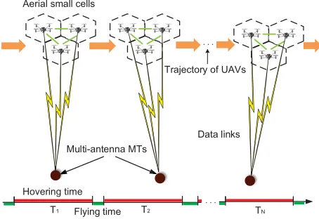
We consider a general UAV swarm-enabled small cell net-work, as shown in Fig. 1. To control the cost of UAV communications [1], we assume the swarm consists of K
single-antenna UAVs. Each UAV acts as an aerial small cell BS, and all UAVs in the swarm serve N MTs in a coor-dinated manner. Specifically, the UAV swarm works in an energy-efficient hover-to-transmit mode [15], [16], which means that the aerial small cells will hover at the MT for some time to serve it and then fly to the next MT. Without loss of generality, each MT is assumed to haveM receive antennas, so that the received signal of then-th MT can be expressed as
FIGURE 1. Illustration of the UAV swarm-enabled small cell network.
We consider the realistic UAV channel model [26], where the channel matrix is given by
Hn=SnLn, n=1∼N. (2) In (2),Sn ∈ CM×K whose elements are i.i.d. standard com-plex Gaussian random variables. These variables describe the fast fading caused by NLOS multi-path components. Besides,
Ln = diag
ln,1, . . . ,ln,K ∈ CK×K is a diagonal matrix. According to [26], we have
ln,k =dn−2,k10−
δn,k
10 , n=1∼N, k=1∼K (3) wheredn,kdenotes the distance between then-th MT and the
k-th UAV, andδn,kcan be expressed as
δn,k=
A
1+ae−b(θn,k−a)
+B, n=1∼N, k=1∼K (4) whereA = ηLOS−ηNLOS,B = 20log10(4πf/c)+ηNLOS,
ηLOS, ηNLOS, a, b are parameters related to the channel
environment and assumed to be constant forN MTs,θn,k =
180
π arccos(hn,k/dn,k) andhn,k denotes the height of the UAV. These parameters can be regarded as slowly-varying LOS components in the radio propagation.
We assume both the trajectory of UAVs and the locations of MTs are known prior to the flight [15], [16], [25]. Hence, we can use the position-related large-scale CSIT for EE opti-mization, i.e.Lnin (2). On the other hand,Snvaries fast and can not be precisely acquired by the UAVs [25]. We assume the transmitter only knows the distribution ofSn.
It is worth noting that both the transmit power and the hov-ering time of UAVs are pre-scheduled prior to the flight [24]. Denoting pn,k as the transmit power of the k-th UAV for the n-th MT, and Tn as the hovering time of the UAV swarm for the n-th MT, we can describe the total energy consumption as [28]
E(P,T)=c
N
X
n=1
K
X
k=1 Tn
pn,k
ηk
+PindTtotal (5)
where P = {P1, . . . ,PN} denotes the set of transmit power, Pn = diag
pn,1, . . . ,pn,K is the diagonal power
matrix, T = (T1, . . . ,TN)T denotes the hovering time of the UAV swarm, c is the power loss coefficient, ηk describes the power amplifier efficiency of the k-th UAV,
Pinddenotes the transmission-power-independent power con-sumption (e.g. the average propulsion power concon-sumption), usually regarded as constant [25], [28], andTtotaldenotes the total hovering time. Accordingly, the total data size transmit-ted by the UAV swarm is written as [25]
D(P,T)=
N
X
n=1
Tnlog2det
In+
1
σ2SnLnPnL
H nSHn
. (6)
Due to the fast moving of UAVs, it is challenging to acquire the instantaneous CSIT (i.e. Sn). Therefore, we use the
ergodictotal data size to calculate EE,
η(P,T)=ES{D(P,T)}
E(P,T) (7)
where η(P,T) is the EE of UAV communication,
ES{D(P,T)}denotes the ergodic total data size, which has
been averaged over all possible realizations ofS, whereS= {S1, . . . ,SN}is the set of small-scale channel parameters.
In UAV networks, the optimization of EE is limited by practical constraints, such as the on-board energy of each UAV. Denoting the maximum transmit energy of the
k-th UAV as Ek, the transmit energy constraints can be formulated as
N
X
n=1
Tnpn,k ≤Ek, k=1∼K (8)
whereTnandpn,kare defined in (5). Moreover, limited by the performance of on-board devices [1], the transmit power of UAVs is upper bounded. We can derive the power constraints of the UAVs as
0≤pn,k ≤pmax, n=1∼N, k=1∼K (9) wherepmaxdenotes the maximum transmit power of a single UAV.
Another constraint that needs to be considered is the UAV hovering time, due to the limitations of the UAV flight [8], [16]. Specifically, both the total hovering time and the maxi-mum hovering time of the UAV swarm at each MT should be considered. The constraints can be formulated as
N
X
n=1
Tn ≤Ttotal (10)
0≤Tn ≤Tmax, n=1∼N (11)
whereTtotaldenotes the total hovering time of UAVs during the flight,Tmaxdenotes the maximum hovering time of UAVs when serving a MT.
Based on (5)–(11), the EE maximization problem now can be formulated as
max
s.t.
N
X
n=1
Tn≤Ttotal (12b)
N
X
n=1
Tnpn,k ≤Ek, k=1∼K (12c)
0≤pn,k ≤pmax, n=1∼N, k=1∼K (12d)
0≤Tn≤Tmax, n=1∼N (12e)
where the value of the parameters in (12b)–(12e) (e.g.pmax,
Ek, etc.) are determined by the design of UAVs and the service demand of MTs [25].
It is worth noting that expectation is involved in the objec-tive function in (12a). Moreover,PandTare coupled in (12c). These facts indicate that the problem (12) is difficult to be solved directly. In the next section, we will propose fea-sible simplifications and effective algorithms to solve this problem.
III. EE OPTIMIZATION SCHEME A. PROBLEM APPROXIMATION
We utilize the techniques proposed in [25] to sim-plify (12). We first formulate a new objective function
Da(P,T,w), which can closely approximate ES{D(P,T)}
without expectation,
Da(P,T,w)= N X n=1 K X k=1
Tnlog2 1+
Mln2,kpn,k
wnσ2
! +M N X n=1 Tn h
log2(wn)−log2e(1−w−1n )i (13)
wherew=(w1, . . . ,wN)T is a set of slack variables,
wn=1+ K
X
k=1
ln2,kpn,k
σ2+Ml2
n,kpn,kw−1n
, n=1∼N. (14)
Using (13), the original EE maximization problem is transformed to
max
P,T ηa(
P,T,w) (15a)
s.t.
N
X
n=1
Tn≤Ttotal (15b)
N
X
n=1
Tnpn,k ≤Ek, k=1∼K (15c)
0≤pn,k ≤pmax, n=1∼N, k=1∼K (15d)
0≤Tn≤Tmax, n=1∼N (15e)
wn=1+ K
X
k=1
ln2,kpn,k
σ2+Ml2
n,kpn,kw
−1
n
, n=1∼N
(15f)
where
ηa(P,T,w)=
Da(P,T,w)
E(P,T) (16)
and the new constraint (15f) is introduced by the coupling betweenPandw. In fact,wcan be regarded as an implicit function with respect toP.
B. PROBLEM DECOMPOSITION
The new problem (15) is a nonlinear fractional optimization problem, which is non-convex due to the coupling between
PandT. To solve this problem, we decompose (15) into two subproblems. In the first subproblem,Pis the optimization variable andTis regarded as constant. Its solution is referred to as the coordinated power allocation strategy. In the second subproblem,Tis the optimization variable andPis regarded as constant. Its solution is referred to as the hovering time scheduling strategy.
Denoting the iteration index asi, the two subproblems at thei-th step can be respectively formulated as
max
Pi ηa(P
i,Ti−1,wi) (17a)
s.t.
N
X
n=1
Tni−1pin,k ≤Ek, k=1∼K (17b)
0≤pi
n,k ≤pmax, n=1∼N, k=1∼K (17c)
win=1+
K
X
k=1
ln2,kpin,k
σ2
m+Mln2,kp i
n,k(win)−1
, n=1∼N
(17d)
and
max
Ti ηa(P
i,Ti,wi) (18a)
s.t.
N
X
n=1
Tni ≤Ttotal (18b)
N
X
n=1
pin,kTni≤Ek, k=1∼K (18c)
0≤Tni ≤Tmax, n=1∼N (18d)
The solutions to (17) and (18) will be given in Section III.C and Section III.D, respectively.
C. COORDINATED POWER ALLOCATION
In this subsection, we derive the solution to (17). Actu-ally, (17) is a nonlinear fractional optimization problem, which is non-convex [29]. According to [30], (17) can be transformed to a convex optimization problem as
max
Pi Da(
Pi,Ti−1,wi)−γpE(Pi,Ti−1) (19a)
s.t.
N
X
n=1
Tni−1pin,k ≤Ek, k=1∼K (19b)
0≤pin,k ≤pmax, n=1∼N, k=1∼K (19c)
win=1+
K
X
k=1
ln2,kpin,k
σ2
m+Mln2,kpni,k(win)−1
, n=1∼N
where
γp=
Da(Pi∗,Ti−1,wi∗)
E(Pi
∗,Ti−1)
(20)
and Pi∗ is the optimal solution to (17) at the i-th step, Ti−1 is regarded as constant at the i-th step, wi∗ is derived
using (19d).
However, the value ofPi
∗ cannot be obtained unless (17)
is solved, which means the value ofγpis actually unknown in (19). Hence, we propose an algorithm to findγp andPi∗
iteratively. Denoting the iteration index as j, the problem in (19) at thej-th step can be expressed as
max
Pj Da(P
j,Ti−1,wj)−γj−1
p E(Pj,Ti−1) (21a)
s.t.
N
X
n=1
Tni−1pjn,k≤Ek, k=1∼K (21b)
0≤pjn,k≤pmax, n=1∼N, k=1∼K (21c)
wjn=1+
K
X
k=1
ln2,kpjn,k
σ2
m+Mln2,kp j n,k(w
j n)−1
. n=1∼N.
(21d)
This method is summarized in Algorithm 1, and the conver-gence can be guaranteed according to [30].
Algorithm 1Iterative Algorithm to Solve (21)
Input:{Ek,k=1∼K},pmax,Ti−1.
1: Initialization:=1×10⁻³,j=1,γp0=0;
2: Solve (21), denoting the optimal solution isP∗, setP1=
P∗;
3: While|Da(Pj,Ti−1,wj)−γpj−1E(Pj,Ti−1)|> do
4: γpj=Da(Pj,Ti−1,wj)/E(Pj,Ti−1)
5: j=j+1;
6: Solve (21), denoting the optimal solution isP∗, set
Pj=P∗;
Output: Pj.
Although (21) is convex [27], it is computationally expen-sive to solve this problem directly, due to the coupling betweenPandwin (21d). To reduce the complexity, we sub-stitutewwithv=(v1, . . . ,vN)T as
wn=evn, n=1∼N. (22) Such substitution is feasible for the reason thatwnis positive for allnaccording to (14). Then, (21) can be reformulated as
max
Pj minv f(P
j,Ti−1,v) (23a)
s.t.
N
X
n=1
Tni−1pjn,k ≤Ek, k=1∼K (23b)
0≤pj
n,k ≤pmax, n=1∼N, k=1∼K (23c)
vn≥0, n=1∼N (23d)
where
f(Pj,Ti−1,v)=XN
n=1
XK
k=1T
i−1
n log2 1+
Mln2,kpjn,k
evnσ2
m
!
+Mlog2eXN
n=1T
i−1
n vn+e−vn−1
−γj−1
p E(P
j,Ti−1). (24)
The equivalence between (21) and (23) can be proved on the basis of the following proposition.
Proposition 1: Whenwsatisfies (14), the correspondingv
is the extreme point off(Pj,Ti−1,v) with respect tov.
Proof: We can derive the first-order derivative of
f(Pj,Ti−1,v) with respect tovas
∂f
∂vn
= MT
i−1
n ln 2 (−
K
X
k=1
ln2,kpjn,ke−vn
σ2
m+Mln2,kp j n,ke−vn
−e−vn +1), n=1∼N. (25) Based on (25), we can find the extreme point off(Pj,Ti−1,v) when ∂∂vnf =0, so that we have
K
X
k=1
ln2,kpjn,ke−vn
σ2
m+Ml2n,kp j n,ke−vn
+e−vn −1=0, n=1∼N (26)
which can be further rewritten as
evn =1+
K
X
k=1
ln2,kpjn,k
σ2
m+Mln2,kp j n,ke−vn
, n=1∼N. (27)
Note that we havewn =evn forn =1 ∼N. Hence, (27) is
equivalent to (14).
In (24), it is easy to find thatf(Pj,Ti−1,v) is convex with respect tov. As a result, the minimum value off(Pj,Ti−1,v)
is achieved at the extreme point with respect to v. Based on Proposition1, the equivalence between (21) and (23) is proved.
Moreover, we can observe thatf(Pj,Ti−1,v) is concave
with respect toPj. According to [31], the optimal solution is a saddle point off(Pj,Ti−1,v). As a result, (23) can be solved in an iterative way after being decomposed into two subprob-lems. Denoting the iteration index ast, the subproblems at thet-th step can be formulated as
max
Pt f(P
t,Ti−1,vt−1) (28a)
s.t.
N
X
n=1
Tni−1ptn,k ≤Ek, k=1∼K (28b) 0≤ptn,k≤pmax, n=1∼N, k=1∼K (28c) and
min
vt f(P
t,Ti−1,vt) (29a)
Algorithm 2Iterative Algorithm to Solve (23)
Input:{Ek,k=1∼K},pmax,Ti−1,γpj−1.
1: Initialization:=1×10⁻³,t=1,P0=0,v0=0;
2: Solve (28), denoting the optimal solution is P∗, set
P1=P∗;
3: Solve (29), denoting the optimal solution is v∗, set
v1=v∗;
4: While|f(Pt,Ti−1,vt)−f(Pt−1,Ti−1,vt−1)|> do 5: t=t+1;
6: Solve (28), denoting the optimal solution isP∗, set
Pt =P∗;
7: Solve (29), denoting the optimal solution isv∗, set vt =v∗;
Output: Pt.
whereTi−1andγj−1
p in (24) are regarded as constants. This scheme is summarized in Algorithm 2, and its convergence is guaranteed according to [27, Theorem 2]. Recalling that the objective function is convex with respect tovt and concave with respect to Pt, both (28) and (29) can be solved using conventional convex optimization tools [29].
D. HOVERING TIME SCHEDULING
As (18) is similar to (17), it can be solved following the same line of reasoning as Algorithm 1. However, the computational complexity of the iterative algorithm is large. To address this problem, we propose a scheme to solve (18) directly.
It is easy to find that (18) is a linear fractional opti-mization problem with linear constraints. According to [29, Section 4.3.2], the optimal solution to a linear fractional optimization problem can be derived based on the solution to a linear optimization problem, after a slack variable is introduced. The linear optimization problem is written as
max
Ti,z Da(P
i,Ti,wi) (30a)
s.t.
N
X
n=1
K
X
k=1 pin,k
ηk
Tni+PindTtotalz=1 (30b) N
X
n=1
Tni−Ttotalz≤0 (30c)
N
X
n=1
pin,kTni−Ekz≤0, k=1∼K (30d)
Tni−Tmaxz≤0, n=1∼N (30e)
z≥0 (30f)
Tni≥0, n=1∼N (30g)
where Pi and wi can be regarded as constants which sat-isfy (14), andzis the introduced slack variable. According to [29], the solution to (18) can be derived based on the solution to (30).
Before discussing the relationship between (18) and (30), we firstly introduce a property of (30).
Proposition 2: Denoting the optimal solution to (30) as (T∗,z∗), we havez∗>0.
Proof: Based on (30g), we only need to prove that
z∗ 6= 0. If z∗ = 0, we will have T∗ = 0 according to (30e) and (30f). Note that (T∗,z∗) must satisfy the con-straint in (30b). If we substitutez∗=0 andT∗=0into (30b), we will have 0 = 1, which is contradict to the original assumption thatz∗=0. As a result,z∗>0 is given. The conclusion of Proposition2 shows that we can cal-culate 1/z∗without any discussions, because the value ofz∗
is always positive. Based onProposition2, we can give the optimal solution to (18), which will be shown in the following proposition.
Proposition 3: The optimal solution to (18) isT∗/z∗. Proof: Firstly, we claim thatT∗/z∗ is a feasible solu-tion to (18). The reason is that according to (30c)–(30g), (18b)–(18d) are satisfied byT∗/z∗obviously, so thatT∗/z∗
is a feasible solution to (18).
Denoting the optimal solution to (18) asTˆ, we definezˆ=
1/E(Pi,Tˆ). Then, substituting (Tˆzˆ,ˆz) into (30), we can find that (Tˆˆz,zˆ) is a feasible solution to (30). Due to the optimality ofT∗in (30), we have
Da(Pi,T∗,wi)≥Da(Pi,Tˆˆz,wi). (31) As (Tˆˆz,zˆ) is a feasible solution to (30) which satisfies (30b), we have
Da(Pi,Tˆˆz,wi)=
Da(Pi,Tˆˆz,wi)
cPN
n=1
PK
k=1Tˆnˆzpnη,k
k +PindTtotalˆz
= Da(P
i,Tˆ,wi)
E(Pi,Tˆ) (32)
and
Da(Pi,T∗,wi)=
Da(Pi,T∗,wi)
cPN n=1
PK k=1Tn∗
pn,k
ηk +PindTtotalz
∗
= Da(P
i,T∗/z∗,wi)
E(Pi,T∗/z∗) (33)
because (T∗,z∗) also satisfies (30b). Hence, we have
Da(Pi,T∗/z∗,wi)
E(Pi,T∗/z∗) ≥
Da(Pi,Tˆ,wi)
E(Pi,Tˆ) (34)
according to (31), which meansT∗/z∗is the optimal solution
to (18).
UsingProposition2andProposition3, we can derive the optimal solution to (18) after the optimal solution to (30) is given. As shown in (13) and (30a)–(30g), (30) is a linear optimization problem. Such problem can be directly solved using conventional linear optimization tools [29].
Algorithm 3Proposed EE Optimization Algorithm
Input:{Ek,k=1∼K},Ttotal,pmax,Tmax
1: Initialization: = 1×10⁻⁴,i = 1,T0 =(Ttotal/N)1,
P0=0;
2: Solve (17), denoting the optimal solution isP∗, setP1=
P∗;
3: While|ηa(Pi,Ti−1,wi)−ηa(Pi−1,Ti−1,wi−1)|> do 4: Solve (18), denoting the optimal solution isT∗, set
Ti=T∗; 5: i=i+1;
6: Solve (17), denoting the optimal solution isP∗, set Pi=P∗;
Output: Pi,Ti.
IV. SIMULATION RESULTS
In this section, we evaluate the proposed EE maximization scheme through simulations. We assume each MT equips withM =6 receive antennas, the number of UAVs in a swarm is set asK =6 and the number of MTs is set asN =10. For the channel parameters, we setf =2 GHz,c=3×10⁸m/s,
ηLOS=0.1,ηNLOS=21,a=5.0188,b=0.3511 according
[image:7.576.301.533.180.361.2]to [26],dn,kandhn,kare randomly generated but are fixed in each realization. The noise power is set asσ2= −107 dBm. Regarding the total energy in (5), we setc=2.63,ηk =0.08 fork = 1 ∼K,Pind =20 dB [28]. We set the power limit of a UAV aspmax =300 mW [25]. Without loss of fairness, we assume the UAVs have the sameEk fork=1∼K, and the sum ofEk is denoted asEtotal.
FIGURE 2. Convergence performance of the proposed EE optimization algorithm, shown by the distribution of iteration times.
In Fig. 2, we evaluate the convergence performance of the proposed EE optimization algorithm. In this simulation, we set Ttotal = 100 s,Tmax = 15 s and the total transmit energy (i.e.Etotal) is set as 30 J. These parameters are applied for all the subsequent simulations, unless otherwise specified. The proposed algorithm has been tested over 100 snapshots,
where for every snapshot the positions of the UAVs and the users are randomly and independently generated. According to the results, the algorithm needs 2.77 iterations on average to converge. To demonstrate the convergence performance, we show the distribution of the iteration times by the his-togram. The result shows that the convergence performance of the proposed algorithm can be guaranteed for practical UAV swarm-enabled small cell networks.
FIGURE 3. The EE of communication when the total transmit energy of UAVs is different, varying with the number of UAVs.
In Fig. 3, we discuss the influence of UAV swarm size on the EE performance. It is observed that when the swarm size increases (while keeping the total transmit energy fixed), a better EE performance is achieved. One reason for this phenomenon is that a higher diversity gain can be obtained with more UAVs in a swarm. Moreover, the coordination of aerial small cells is more flexible with larger swarm size, which leads to a better performance of EE. Besides, the EE performance cannot be infinitely improved by increasing the UAV swarm size, because the transmit energy of each UAV is less with larger swarm size. We further observe that the EE is saturated at high transmit energy. The reason is that the transmit power of most UAVs will reach the upper bound in this case. Hence, the EE can hardly be further improved by increasing the transmit energy.
[image:7.576.46.270.441.622.2]FIGURE 4. The EE of communication with different maximum hovering time of a single UAV, varying with the total transmit energy of UAVs.
exists a tradeoff between the user number and EE in UAV swarm-enabled small cell networks.
FIGURE 5. The EE of communication when the total transmit energy of UAVs is different, varying with the number of MTs.
[image:8.576.301.531.69.246.2]In Fig.5, we further discuss the influence of user number on the EE. It is observed that the increasing number of MTs has a positive influence on the EE performance, for the reason that more MTs with better channel condition can be chosen to serve by UAVs. In other words, after the MTs are sched-uled by the proposed algorithm, the MTs with bad channel condition are not served by UAVs. This result shows that the tradeoff between the user number and EE actually exists in UAV swarm-enabled small cell networks when the total transmit energy is fixed, as analyzed in Fig.4. Furthermore, we can observe that increasing the total transmit energy is a better way to improve the EE performance with larger number of MTs, which implies that the transmit energy is a critical bottleneck for UAV swarm-enabled small cell networks.
FIGURE 6. The EE of communication with different power limit of UAVs, varying with the total transmit energy of UAVs.
In Fig.6, the influence of power limit on the EE perfor-mance is evaluated. It is observed that the EE increases with larger power limit. Similar to the analysis in Fig.4, the reason for this phenomenon is that higher EE can be achieved when the feasible region of the EE maximization problem is larger. We can also observe that the curves are close to each other when the maximum transmit power is 100 mW and 300 mW. This is because part of performance loss can be compensated by hovering time scheduling when the transmit power is low. Such performance loss is hard to be compensated by hovering time scheduling when the transmit power is high, because the total transmit energy is limited.
FIGURE 7. The EE of communication with different total hovering time of UAVs, varying with the total transmit energy of UAVs.
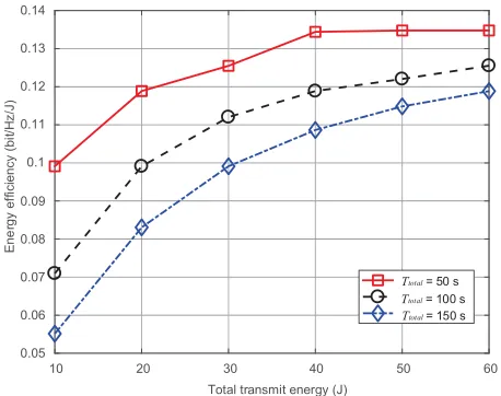
[image:8.576.43.272.339.520.2] [image:8.576.303.532.463.644.2]and 22.5 s respectively. As shown by the simulation results, reducing the total hovering time leads to higher EE. The reason is that the transmit power of UAVs is generally higher when the total transmit energy is consumed in a shorter time. In this case, higher EE is achieved due to higher transmit power.
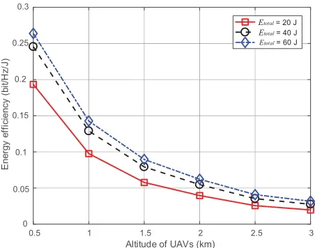
FIGURE 8. The EE of communication when the total transmit energy of UAVs is different, varying with the altitude of UAVs.
In Fig.8, we demonstrate the EE with varying altitudes of UAVs. Specifically, we sethn,k = hU +300φn,k, where
φn,k are uniformly distributed variables in the range of [0,1] m, andhU changes from 0.5 km to 3 km. As demonstrated by the curves, we can observe that a higher EE can be achieved and the EE can be better improved by increasing the transmit power, when the altitude of UAVs is lower. The reason is that channel fading is less severe when the UAVs are hovering at a lower altitude. In this case, the total data size can become larger when the total energy consumption remains unchanged, which means a better performance can be achieved. On the other hand, the low altitude of UAVs results in a limited coverage area. These results imply that there exists a tradeoff between the coverage area and EE in UAV swarm-enabled small cell networks.
[image:9.576.44.270.155.333.2]In Fig. 9, we compare the proposed algorithm with the conventional algorithm, which allocates the transmit power and hovering time of UAVs equally between the MTs, and the algorithm in [25]. We can observe that the EE increases with the total transmit energy, as a larger transmit energy can provide higher degrees of freedom for EE optimization. More importantly, it is shown that the proposed algorithm outperforms other schemes on the regime of transmit energy. When the transmit energy is lower than 30 J, the proposed algorithm has a similar performance to the algorithm in [25]. The reason is that the total energy consumption is nearly a constant when the transmit energy is much lower than the transmission-energy-independent energy consumption. In this case, the optimization of total data size is similar to the optimization of EE. When the transmit energy becomes
FIGURE 9. The EE of communication using different optimization algorithms, varying with the total transmit energy of UAVs.
higher, the gap between the proposed algorithm and other algorithms becomes larger. The results indicate that optimiz-ing the EE is important for the UAV swarm-enabled small cell network, especially with high transmit energy.
V. CONCLUSION
In this paper, we have investigated the optimization of EE for UAV swarm-enabled small cell networks with large-scale CSIT, considering the coordination of aerial small cells under energy constraints. The EE maximization problem has been formulated, which is a non-convex fractional optimization problem and hard to be solved directly. We have decom-posed it into two subproblems, which can be efficiently solved by the proposed iterative algorithm. Simulation results have demonstrated that it is valuable to jointly consider the coordination of aerial small cells and the large-scale CSIT when optimizing the EE for UAV swarm-enabled small cell networks.
APPENDIX
PROOF OF THE CONVERGENCE OF ALGORITHM 3
Assuming thatPi−1andTi−1are solutions to (17) and (18)
at the (i−1)-th step. After we solve (17), we havePias the optimal solution, which satisfies
ηa(Pi,Ti−1,wi)≥ηa(Pi−1,Ti−1,wi−1). (A.1) Then after (18) is solved at thei-th step, we haveTi as the optimal solution, which satisfies
ηa(Pi,Ti,wi)≥ηa(Pi,Ti−1,wi). (A.2) According to (A.1) and (A.2), we have
given resources. As a result, Algorithm 3 is guaranteed to converge.
REFERENCES
[1] S. Hayat, E. Yanmaz, and R. Muzaffar, ‘‘Survey on unmanned aerial vehi-cle networks for civil applications: A communications viewpoint,’’IEEE Commun. Surveys Tuts., vol. 18, no. 4, pp. 2624–2661, 4th Quart., 2016. [2] B. Li, Z. Fei, and Y. Zhang, ‘‘UAV communications for 5G and beyond:
Recent advances and future trends,’’IEEE Intern. Things J., vol. 6, no. 2, pp. 2241–2263, Apr. 2019. doi:10.1109/JIOT.2018.2887086.
[3] L. Gupta, R. Jain, and G. Vaszkun, ‘‘Survey of important issues in UAV communication networks,’’IEEE Commun. Surveys Tuts., vol. 18, no. 2, pp. 1123–1152, 2nd Quart., 2016.
[4] T. Qi, W. Feng, and Y. Wang, ‘‘Outage performance of non-orthogonal multiple access based unmanned aerial vehicles satellite networks,’’China Commu., vol. 15, no. 5, pp. 1–8, May 2018.
[5] Z. Yuan, J. Jin, L. Sun, K.-W. Chin, and G.-M. Muntean, ‘‘Ultra-reliable IoT communications with UAVs: A swarm use case,’’IEEE Commun. Mag., vol. 56, no. 12, pp. 90–96, Dec. 2018.
[6] Y. Zeng, R. Zhang, and T. J. Lim, ‘‘Wireless communications with unmanned aerial vehicles: Opportunities and challenges,’’ IEEE Commun. Mag., vol. 54, no. 5, pp. 36–42, May 2016.
[7] Y. Zeng and R. Zhang, ‘‘Energy-efficient UAV communication with tra-jectory optimization,’’IEEE Trans. Wireless Commun., vol. 16, no. 6, pp. 3747–3760, Jun. 2017.
[8] M. Mozaffari, W. Saad, M. Bennis, and M. Debbah, ‘‘Mobile unmanned aerial vehicles (UAVs) for energy-efficient Internet of Things communi-cations,’’IEEE Trans. Wireless Commun., vol. 16, no. 11, pp. 7574–7589, Nov. 2017.
[9] C. H. Liu, Z. Chen, J. Tang, J. Xu, and C. Piao, ‘‘Energy-efficient UAV control for effective and fair communication coverage: A deep reinforce-ment learning approach,’’IEEE J. Sel. Areas Commun., vol. 36, no. 9, pp. 2059–2070, Sep. 2018.
[10] Q. Song and F. Zheng, ‘‘Energy efficient multi-antenna UAV-enabled mobile relay,’’China Commun., vol. 15, no. 5, pp. 44–50, May 2018. [11] Z. Zhou, C. Zhang, C. Xu, F. Xiong, Y. Zhang, and T. Umer,
‘‘Energy-efficient industrial Internet of UAVs for power line inspection in smart grid,’’IEEE Trans. Ind. Informat., vol. 14, no. 6, pp. 2705–2714, Jun. 2018. [12] M. B. Ghorbel, H. Ghazzai, A. Kadri, M. J. Hossain, and H. Menouar, ‘‘An energy efficient overlay cognitive radio approach in UAV-based com-munication,’’ inProc. IEEE GLOBECOM, Abu Dhabi, UAE, Dec. 2018, pp. 1–6.
[13] H. Shakhatreh, A. Khreishah, J. Chakareski, H. B. Salameh, and I. Khalil, ‘‘On the continuous coverage problem for a swarm of UAVs,’’ inProc. IEEE 37th Sarnoff Symp., Newark, NJ, USA, Sep. 2016, pp. 130–135. [14] L. Ruan, J. Wang, J. Chen, Y. Xu, Y. Yang, H. Jiang, Y. Zhang, and
Y. Xu, ‘‘Energy-efficient multi-UAV coverage deployment in UAV net-works: A game-theoretic framework,’’China Commun., vol. 15, no. 10, pp. 194–209, Oct. 2018.
[15] M. Monwar, O. Semiari, and W. Saad, ‘‘Optimized path planning for inspection by unmanned aerial vehicles swarm with energy constraints,’’ inProc. IEEE GLOBECOM, Abu Dhabi, UAE, Dec. 2018, pp. 1–6. [16] H. Ghazzai, M. B. Ghorbel, A. Kassler, and J. Hossain, ‘‘Trajectory
optimization for cooperative dual-band UAV swarms,’’ inProc. IEEE GLOBECOM, Abu Dhabi, UAE, Dec. 2018, pp. 1–7.
[17] M. Chen, F. Dai, H. Wang, and L. Lei, ‘‘DFM: A distributed flocking model for UAV swarm networks,’’IEEE Access, vol. 6, pp. 69141–69150, 2018.
[18] Q. Zhang, M. Jiang, Z. Feng, W. Li, W. Zhang, and M. Pan, ‘‘IoT enabled UAV: Network architecture and routing algorithm,’’IEEE Intern. Things J., vol. 6, no. 2, pp. 3727–3742, Apr. 2019. doi:10.1109/JIOT.2018.2890428. [19] R. K. Patra and P. Muthuchidambaranathan, ‘‘Optimisation of spectrum and energy efficiency in UAV-enabled mobile relaying using bisection and PSO method,’’ inProc. IEEE I2CT, Pune, India, Apr. 2018, pp. 1–7. [20] A. M. Koushik, F. Hu, and S. Kumar, ‘‘Deep Q-Learning based node
posi-tioning for throughput-optimal communications in dynamic UAV swarm network,’’IEEE Trans. Cognit. Commun. Netw., to be published. doi:10. 1109/TCCN.2019.2907520.
[21] N. Lu, Y. Zhou, C. Shi, N. Cheng, L. Cai, and B. Li, ‘‘Planning while flying: A measurement-aided dynamic planning of drone small cells,’’
IEEE Internet Things J., vol. 6, no. 2, pp. 2693–2705, Apr. 2019.
[22] S.-F. Chou, Y.-J. Yu, A.-C. Pang, and T.-A. Lin, ‘‘Energy-aware 3D aerial small-cell deployment over next generation cellular networks,’’ inProc. IEEE VTC-Spring, Porto, Portugal, Jun. 2018, pp. 1–5.
[23] A. A. Khuwaja, G. Zheng, Y. Chen, and W. Feng, ‘‘Optimum deployment of multiple UAVs for coverage area maximization in the presence of co-channel interference,’’IEEE Access, vol. 7, pp. 85203–85212, 2019. [24] M. Mozaffari, W. Saad, M. Bennis, and M. Debbah, ‘‘Wireless
communica-tion using unmanned aerial vehicles (UAVs): Optimal transport theory for hover time optimization,’’IEEE Trans. Wireless Commun., vol. 16, no. 12, pp. 8052–8066, Dec. 2017.
[25] W. Feng, J. Wang, Y. Chen, X. Wang, N. Ge, and J. Lu, ‘‘UAV-aided MIMO communications for 5G Internet of Things,’’IEEE Internet Things J., vol. 6, no. 2, pp. 1731–1740, Apr. 2019.
[26] Y. Chen, W. Feng, and G. Zheng, ‘‘Optimum placement of UAV as relays,’’
IEEE Commun. Lett., vol. 22, no. 2, pp. 248–251, Feb. 2018.
[27] W. Feng, Y. Wang, N. Ge, J. Lu, and J. Zhang, ‘‘Virtual MIMO in multi-cell distributed antenna systems: Coordinated transmissions with large-scale CSIT,’’IEEE J. Sel. Areas Commun., vol. 31, no. 10, pp. 2067–2081, Oct. 2013.
[28] J. Joung, Y. K. Chia, and S. Sun, ‘‘Energy-efficient, large-scale distributed-antenna system (L-DAS) for multiple users,’’IEEE J. Sel. Topics Signal Process., vol. 8, no. 5, pp. 954–965, Oct. 2014.
[29] S. Boyd and L. Vandenberghe,Convex Optimization. Cambridge, U.K.: Cambridge Univ. Press, 2004.
[30] W. Dinkelbach, ‘‘On nonlinear fractional programming,’’Manage. Sci., vol. 13, no. 7, pp. 492–498, Mar. 1967.
[31] W. Murray and M. L. Overton, ‘‘A projected Lagrangian algorithm for nonlinear minimax optimization,’’SIAM J. Sci. Stat. Comput., vol. 1, no. 3, pp. 345–370, Sep. 1980.
CHENGXIAO LIU received the B.S. degree from the Department of Electronic Engineering, Tsinghua University, Beijing, China, in 2017, where he is currently pursuing the Ph.D. degree. His research interests include maritime commu-nications, hybrid satellite-terrestrial networks, and UAV communications.
JUE WANG (S’10–M’14) received the B.S. degree in communications engineering from Nan-jing University, NanNan-jing, China, in 2006, and the M.S. and Ph.D. degrees from the National Communications Research Laboratory, Southeast University, Nanjing, China, in 2009 and 2014, respectively. From 2014 to 2016, he was with the Singapore University of Technology and Design as a Postdoctoral Research Fellow. He is currently with the School of Electronic and Information Engineering, Nantong University, Nantong, China. His research interests include MIMO wireless communications, multiuser transmission, MIMO channel modeling, massive MIMO systems, and physical layer security. He has served as a Technical Program Committee Member for a number of the IEEE conferences and a Reviewer for the various IEEE journals. He was awarded as an Exemplary Reviewer of the IEEE TRANSACTIONS ON COMMUNICATIONS, in 2014.
YUNFEI CHEN (S’02–M’06–SM’10) received the B.E. and M.E. degrees in electronic engineer-ing from Shanghai Jiao Tong University, China, in 1998 and 2001, respectively, and the Ph.D. degree from the University of Alberta, Canada, in 2006. He is currently with the School of Engi-neering, University of Warwick, Coventry, U.K. His research interests include energy harvesting, wireless relaying and general performance analy-sis, and design of wireless systems.