A Path-Oriented Encoding Evolutionary Algorithm for Network
Coding Resource Minimization
Huanlai Xing1, Rong Qu1, Graham Kendall1,2, and Ruibin Bai3 1
University of Nottingham, Nottingham, UK; 12
University of Nottingham, Malaysia Campus; 3
University of Nottingham Ningbo, Ningbo, China
Abstract
:
Network coding is an emerging telecommunication technique, where any intermediate node is allowed to recombine incoming data if necessary. This technique helps to increase the throughput, however, very likely at the cost of huge amount of computational overhead, due to the packet recombination performed (i.e. coding operations). Hence, it is of practical importance to reduce coding operations while retaining the benefits that network coding brings to us.
In this paper, we propose a novel evolutionary algorithm (EA) to minimize the amount of coding operations involved. Different from the state-of-the-art EAs which all use binary encodings for the problem, our EA is based on path-oriented encoding. In this new encoding scheme, each chromosome is represented by a union of paths originating from the source and terminating at one of the receivers. Employing path-oriented encoding leads to a search space where all solutions are feasible, which fundamentally facilitates more efficient search of EAs. Based on the new encoding, we develop three basic operators, i.e. initialization, crossover and mutation. In addition, we design a local search operator to improve the solution quality and hence the performance of our EA. The simulation results demonstrate that our EA significantly outperforms the state-of-the-art algorithms in terms of global exploration and computational time.
Keywords
:
1. Introduction
Network coding is a new routing paradigm, where each intermediate node is not only able to forward the incoming data but also allowed to mathematically recombine (code) them if necessary (Ahlswede et al, 2000; Li et al, 2003). In essence, by introducing extra computations at intermediate nodes, network coding can efficiently make use of the bandwidth resource of a network and accommodate more information flows than traditional routing (Li et al, 2003). Multicast is a routing scheme for one-to-many data transmission, where the same information is delivered from a source to a set of receivers simultaneously (Miller, 1998). When applied in multicast, network coding can always guarantee a theoretically maximal throughput (Ahlswede et al, 2000; Li et al, 2003). However, performing coding operations will consume extra computational overhead and buffers. Hence, a natural concern is how to route the data from the source to all receivers at the expected data rate while minimizing the number of coding operations necessarily performed.
The above problem is NP-hard (Kim et al, 2006) and a number of evolutionary algorithms (EAs) have been proposed (see Section 2.2), where all of them adopt binary encodings to represent chromosomes (see Section 3.2). However, it is observed in this paper that a major weakness of these encodings is that the search space will include a large proportion of infeasible solutions. These solutions are potential barriers during the search and may significantly deteriorate the performance of EAs. This motivates us to investigate a more suitable encoding approach for EAs to effectively address the problem concerned.
In telecommunications, EAs are widely used as an optimizer to select appropriate routes within limited time. When designing EAs, path-oriented encoding is a direct and natural choice since routing itself is to select paths in a network along which the traffic is delivered. In the literature, path-oriented encoding has been adopted by EAs for solving shortest path routing and multicast routing problems. A number of GAs (Ahn and Ramakrishna, 2002; Cheng and Yang, 2010; Yang et al, 2010a) are employed to find the cost-optimal path connecting the given source and receiver. Each chromosome is represented by a path containing a string of IDs of nodes through which the path passes. Also, EAs are used to construct least-cost spanning trees, where each chromosome is represented by a set of paths from the source to receivers (Palmer and Kershenbaum, 1994; Siregar et al, 2005; Oh et al, 2006; Cheng and Yang, 2008, 2010b). Similar to construct a spanning tree, network coding based multicast (NCM) finds a subgraph which owns multiple paths. Hence, path-oriented encoding could be a potential choice as the chromosome representation to the network coding resource minimization problem. However, to our knowledge no research in the literature concerns path-oriented encoding for the problem concerned.
results show that the path-oriented encoding EA is capable of finding optimal solutions in most of the test instances within a very short time, and the proposed EA outperforms the existing EAs due to the new encoding and the well-designed associated operators.
2. Problem Formulation and Related Work
2.1 Problem Formulation
In this paper, a communication network is modeled as a directed graph G = (V, E), where V and E are the node set and link set, respectively. Assume each link eE is with a unit capacity. Only integer flows are allowed in G, hence a link is either idle or occupied by a flow of unit rate (Kim et al, 2007a, 2007b). A network coding based multicast (NCM) request can be defined as a source sV expects to send the same data to a number of receivers T = {t1,…,td}V at rate R, where R is an integer (Xing and Qu, 2012, 2013). Each receiver tT can receive the data sent from the source at rate R (Kim et al, 2007a, 2007b).
Given a NCM request, the task is to find a connected subgraph in G to support the multicast with network coding (Xing and Qu, 2012, 2013). This subgraph is called NCM subgraph (denoted by GNCM). In a NCM subgraph, there are R link-disjoint paths connecting s and each receiver; a coding node is a node that performs coding operations; an outgoing link of a coding node is called a coding link if the data sent out via this link are a combination of the data received by the coding node. In network G, a non-receiver intermediate node with multiple incoming links is referred to as a merging node (Kim et al, 2007a, 2007b). Only merging nodes are possible to become coding nodes. The number of coding links is used to estimate the amount of coding operations performed during the data transmission (Langberg et al, 2006). More descriptions can be found in Xing and Qu (2012). The following lists some notations.
MG: the set of merging nodes in G, where m MG is an arbitrary merging node in G.
Lm: the set of outgoing links of merging node m, where e Lm is an arbitrary outgoing link of node m. σe: a binary variable associated with each link e Lm, m MG. σe = 1 if link e is a coding link; σe = 0 otherwise.
(GNCM): the number of coding links in the NCM subgraph. R(s, tk): the data rate between s and tk in the NCM subgraph. pi(s, tk) : the i-th link-disjoint path from s to tk in GNCM, i = 1,2,…,R.
The network coding resource minimization problem is defined as to find a NCM subgraph with the number of coding links minimized and the data rate R satisfied, shown as follows:
Minimize:
G m
m e
e NCM
G
M L
)
(
Φ
(1)Subject to:
2.2 Related Work
By far, a number of EAs have been proposed for solving the minimization problem. These EAs can be classified into four categories, i.e. genetic algorithms (GAs), estimation of distribution algorithms (EDAs), EAs with efficiency enhancement techniques, and hybridized EAs.
Kim et al developed several GAs to minimize the involved network coding resource. The first GA was only applicable to acyclic networks (Kim et al, 2006). Then, a distributed GA was designed for both acyclic and cyclic networks, where a graph decomposition method (see Section 3.1) was proposed to map the target problem to an EA framework (Kim et al, 2007a). Besides, two binary encoding approaches, i.e. the binary link state (BLS) and the block transmission state (BTS), and their associated operators were evaluated (Kim et al, 2007b) (see Section 3.2).
EDAs have also been used to solve the problem. They maintain one or more probability vectors, rather than a population of explicit solutions. The probability vectors, when sampled, will generate promising solutions with increasingly higher probabilities during the evolution. So far, quantum-inspired evolutionary algorithm (QEAs) and population based incremental learning algorithm (PBIL) have been developed to optimize the problem concerned (Xing et al, 2010; Ji and Xing, 2011; Xing and Qu, 2011a, 2011b).
In addition, Ahn (2011) and Luong et al (2012) studied the minimum-cost network coding problem using evolutionary approaches, where entropy-based evaluation relaxation techniques were introduced to EAs in order to reduce the computational cost incurred during the evolution. By making use of the inherent randomness feature of the individuals, the proposed EAs can rapidly recognize promising solutions with much fewer individuals to be evaluated.
Xing and Qu (2012) proposed a hybridized EA. They designed a local search procedure and incorporated it into the EA framework. Strong global exploration and local exploitation capabilities can both be obtained during the evolution.
Note that all the EAs above adopt binary encodings to represent chromosomes. However, these encodings have their intrinsic drawback as the search space may contain many infeasible solutions which would significantly increase the difficulty of tackling the problem. It is hence worth designing a more appropriate encoding scheme for EAs to effectively address the problem.
3. The Proposed Evolutionary Algorithm
We first review the graph decomposition method based on which the path-oriented encoding is designed. We then review the existing encodings for network coding resource minimization, i.e. the binary link state (BLS) and the block transmission state (BTS). After that, we describe the new encoding, its associated operators and the overall procedure of the proposed EA.
3.1 The Graph Decomposition Method
The graph decomposition method is a means of explicitly showing how information flows pass through merging nodes in network G. This method decomposes each merging node into a number of auxiliary nodes, as described below (Kim et al, 2007a, 2007b).
into two node sets: In(i) incoming auxiliary nodes and Out(i) outgoing auxiliary nodes. Each incoming link of i is redirected to the corresponding incoming auxiliary node and each outgoing link of i is redirected to the corresponding outgoing auxiliary node. In addition, an auxiliary link is inserted between arbitrary pair of incoming and outgoing auxiliary nodes. Fig.1 shows an example of the graph decomposition. The original graph with source s and receivers t1 and t2 is shown in Fig.1(a), where v1 and v2 are merging nodes. Fig.1(b) illustrates the decomposed graph, where eight auxiliary links are inserted, showing all possible routes that information flows may pass through v1 and v2.
(a) Original graph. (b) decomposed graph. Fig.1 An example of graph decomposition.
3.2 The BLS and BTS Encodings
BLS and BTS are the only two existing encoding approaches in the literature for the problem concerned (Kim et al, 2007a, 2007b). They are based on the graph decomposition method. For an arbitrary merging node with In incoming links and Out outgoing links, there are In auxiliary links heading to each outgoing auxiliary node after graph decomposition, e.g. links u1w1 and u2w1 connect w1 and links u1w2 and u2w2 connect w2, as shown in Fig.1(b). Each auxiliary link can be either active or inactive, indicating whether the link allows flow to pass.
Assume there are OAN outgoing auxiliary nodes in the decomposed graph GD, where OAN is an integer. In BLS, a chromosome (solution) X consists of a number of binary arrays bi, i = 1, 2, …, OAN, each determining the states of the auxiliary links heading to a certain outgoing auxiliary node in GD. In BTS, the chromosome representation is the same as that in the BLS encoding. However, for each array bi in BTS-based chromosome, once there are at least two 1’s in bi, the remaining 0’s in bi are replaced with 1’s.
two drawbacks motivate us to devise a more efficient encoding to represent the solutions to the problem concerned.
3.3 The Path-Oriented Encoding and Evaluation
In this paper, we adapt the path-oriented encoding within our proposed EA. Each chromosome consists of a set of paths originating from the source and terminating at one of the receivers. Each path is encoded as a string of positive integers representing the IDs of nodes through which the data passes. The set of paths is classified into d subsets, i.e. d basic unit (BU), where paths in BU connect to the same receiver and they do not share any common link (i.e. they are link-disjoint). Besides, there are R paths in each BU, where R is the expected data rate. Each chromosome is feasible since each BU of the chromosome satisfies the data rate requirement. Each BU can be easily obtained by max-flow algorithms. For example, we find a NCM subgraph from Fig.1(b) which consists of four paths, as shown below.
p1(s,t1) = s→a→t1; p2(s,t1) = s→b→u2→w1→c→u3→w3→t1; p1(s,t2) = s→a→u1→w1→c→u3→w4→t2; p2(s,t2) = s→b→t2;
The corresponding chromosome is illustrated in Fig.2.
Fig.2 An example chromosome
Based on the path-oriented encoding, the chromosome evaluation is simple. For chromosome X, the union of all paths in X forms the corresponding NCM subgraph. The fitness of X, f(X), is known by counting the number of coding links used in the NCM subgraph. So, the computation complexity here is significantly lower than that of BLS and BTS encodings.
Compared with BLS and BTS, path-oriented encoding has two advantages. First, for any instance, the search space consists of feasible solutions only. The absence of infeasible solutions leads to a connected search space, and thus helps to reduce the problem difficulty for EAs. Second, the chromosome evaluation is less time-consuming.
3.4 Initialization
It is widely recognized that, for EAs, a good initial population is more likely to lead to a better optimization result. For the proposed algorithm, we initialize the population in the following way. First, we create an allelic BU pool (pool-i) for each receiver ti, where i = 1,…,d. Second, we randomly choose one BU from pool-i, i = 1,…,d, and combine the selected BUs as a chromosome. The second step is repeated to create a population of a predefined size.
link-disjoint paths) and its volume from s to receiver ti, respectively. The max-flow algorithm (Goldberg, 1985) is used to calculate Flow(s,ti) and Vol(s,ti). Fig.3 shows the initialization procedure of our EA based on the path-oriented encoding.
// Generation of BU pools
1. fori = 1 toddo
2. Set Gtemp = GD and pool-i=
3. forj = 1 topopdo
3. Find Flow(s,ti) from Gtemp by the max-flow algorithm (Goldberg, 1985)
4. ifVol(s,ti) R then
5. Randomly select R paths from Flow(s,ti) as a new BU
6. if the new BU is not in pool-ithen
7. Put this BU into pool-i
8. Set Gtemp = GD
9. Randomly select a BU (with at least one auxiliary link) from pool-i
10. Randomly choose an auxiliary link owned by the selected BU
11. Delete this auxiliary link from Gtemp
// Generation of the population
12. forj = 1 topopdo
13. fori = 1 toddo
14. Randomly select a BU from pool-i
15. Include the BU in the j-th chromosome
16. Output the initial population
Fig.3 The procedure of initialization
For a specific graph Gtemp, only one BU can be obtained by the max-flow algorithm. To obtain an allelic BU pool for receiver ti, we have to change the structure of Gtemp by deleting different links from GD at each time. As aforementioned, how the information flows pass through a given network depends on the states of all auxiliary links in the decomposed network. So, only the auxiliary links are considered for deletion in our EA. To generate a new BU for receiver ti, we randomly pick up a BU from pool-i and randomly select an auxiliary link owned by the BU, as shown in steps 9 and 10. The selected link is then removed from Gtemp to make sure the new Gtemp is different graph.
3.5 Crossover
In the proposed EA, we use single-point crossover to each pair of selected chromosomes with a crossover probability pc. As aforementioned, there are d BUs in a chromosome. The crossover point is randomly chosen from the (d – 1) positions between two consecutive BUs. Two offspring are created by swapping the BUs of the two parents after the crossover point. An example crossover operation is illustrated in Fig.4, where each parent consists of four BUs and the crossover point is between the second and third BUs.
offspring chromosomes so that new regions in search space are explored.
Fig.4 An example of the crossover operator
3.6 Mutation
Mutation is to help the local exploitation and avoid the prematurity of EAs. As mentioned in section 3.3, each BU is a set of R link-disjoint paths from the source to a particular receiver. Mutation upon a BU leads to another set of R link-disjoint paths. The idea behind the mutation is that some auxiliary links owned by the chosen BU are deleted from the secondary graph GD. Then, the new BU is generated by implementing the max-flow algorithm on the new GD. We propose two mutation operators, the ordinary mutation M1 and greedy mutation M2, where each BU of a chromosome is to be mutated with a mutation probability pm. The difference between M1 and M2 is on which links in the chosen BU are deleted. In this paper, we only concern the removal of auxiliary links since they determine the amount of coding resources required.
In M1, for a chosen BU, we randomly select an auxiliary link in the BU and delete the link from the decomposed graph GD. After that, we compute the max-flow, i.e. Flow(s,ti), by using the max-flow algorithm on GD (Goldberg, 1985). If the volume of Flow(s,ti), Vol(s,ti), is not smaller than the expected data rate R, a new BU is obtained by randomly selecting R paths in Flow(s,ti). The new BU then replaces the old BU. If Vol(s,ti) is smaller than R, the data rate requirement cannot be met and the old BU remains. The procedure of M1 is shown in Fig.5, where rnd() generates a random value uniformly distributed in the range [0,1]. Fig.6 shows an example of BU mutation using M1, where the example network G and its decomposed network GD are illustrated in Fig.1. Note that links u2→w1 and u3→w3 are the only auxiliary links in the chosen BU. In the example, link u3→w3 is removed from GD and a new BU is found based on the new GD.
In M1, a random auxiliary link is deleted from GD to compute a new BU. The new BU, combined with the remaining (d – 1) BUs of the chromosome, may lead to an increased number of coding links. This is because no domain knowledge is taken into consideration in M1. To avoid this we propose the greedy mutation M2 which is the same as M1 except the way of which auxiliary links are chosen to be deleted.
1. forj = 1 topopdo
2. fori = 1 toddo
3. ifrnd() < pmthen
// the i-th BU of the j-th chromosome is chosen
4. Set Gtemp = GD
5. if the i-th BU owns at least one auxiliary link then
6. Randomly select an auxiliary link owned by the i-th BU
7. Delete the link from Gtemp
8. Compute Flow(s,ti) from Gtemp using the max-flow algorithm
9. ifVol(s,ti) R then
10. Randomly select R paths from Flow(s,ti) and replace
the old BU with the R paths
11. Output the mutated population
Fig.5 The procedure of the ordinary mutation M1
(a) the chosen BU (b) link deletion from
G
D(c) the new BU
Fig.6 An example of the mutation operator M1
Regarding the mutation probability pm, a fixed value may not be a wise choice since the number of BUs in a chromosome changes according to d, i.e. the number of receivers. A fixed pm value, e.g. 0.1, could lead to a dramatically different number of mutation operations during the evolution, which may not generally applicable for different multicast sessions. In our EA, we set pm = 1/d, thus the amount of mutation operations involved does not change too much in different multicast sessions, hence more likely to lead to a stable optimization performance of EA.
3.7 The Local Search Operator
To enhance local exploitation, we propose a local search (LS) operator which is performed on a randomly selected chromosome at each generation.
redirected to an outgoing auxiliary node after the graph decomposition, as discussed in section 3.1. So in the NCM subgraph of an arbitrary chromosome, each coding link corresponds to a certain coding node (i.e. an outgoing auxiliary node that performs coding). To reduce the number of coding nodes is to decrease the number of coding links. Assume there is a chromosome X of which the NCM subgraph contains K coding nodes, where K is an integer. The LS operator aims to remove the occurrence of coding operation at each coding node. The K coding nodes will be processed one by one, in an ascending order according to their node IDs.
We assume the k-th coding node (denoted by cnode-k, k = 1, 2, …, K) is to be processed by the LS operator. We also assume that there are C (C 2) auxiliary links connecting to cnode-k in the NCM subgraph of X, meaning information via these links is involved in the coding at cnode-k. To remove the coding from cnode-k, one simple idea is to delete arbitrarily (C – 1) auxiliary links from the NCM subgraph of X. However, directly removing these links leads to an infeasible X since BUs which occupy these (C – 1)
links are damaged. To overcome this, our LS operator reconstructs the affected BUs so that they bypass the use of the (C – 1) auxiliary links mentioned above, explained as follows.
First of all, we randomly select (C – 1) auxiliary links connecting to cnode-k and check which BUs are occupying these links. The affected BUs will be reconstructed, while the others remain in the NCM subgraph. Next, we delete the selected (C – 1) auxiliary links from the decomposed graph GD. Besides, we also delete those currently unoccupied auxiliary links from GD which connect to one of the outgoing auxiliary nodes being occupied by the unaffected BUs. The reason to remove the unoccupied auxiliary links is that we expect to reduce the chance of removing one coding node at the expense of introducing other coding node(s). Finally, we reconstruct the affected BUs by using the max-flow algorithm over GD. If all the affected BUs are successfully constructed, we obtain a new chromosome Xnew. If Xnew owns less coding links than X, we replace the incumbent X with Xnew (i.e. the LS moves to an improved solution Xnew) and repeat the LS operator to improve the new incumbent Xnew.Otherwise, we retain X and proceed to the next coding node of
X. The LS operator stops when either no improvement is made to the incumbent chromosome after checking all its coding nodes, or a new chromosome with no coding involved (i.e. optimal) is found.
An example LS is shown in Fig.7, where Fig.1(a) is the example network. The example NCM subgraph GNCM consists of two BUs, i.e. BU1 = {s→a→t1, s→b→u2→w2→d→u4→w3→t1} and BU2 = {s→b→t2, s→a→u1→w2→d→u4→w4→t2}, as seen in Fig.7(a). Obviously, node w2 is the only coding node in GNCM. According to the rule of LS, one of the incoming auxiliary links, i.e. u1→w2 and u2→w2, needs to be removed from GD. In the example, link u1→w2 is chosen for removal and hence the affected BU, i.e. BU2, has to be reconstructed. Besides, as auxiliary nodes w2 and w3 are currently occupied by BU1, all unoccupied auxiliary links heading to w2 and w3 also need to be deleted from GD. So, link u3→w3 is deleted. Based on the new GD, a new BU2 = {s→b→t2, s→a→u1→w1→c→u3→w4→t2} is rebuilt, as shown in Fig.7(c). It is easily seen that the combination of BU1 and BU2 results into a NCM subgraph without coding operation. Hence, the LS procedure stops and returns the resulting NCM subgraph.
(a)
G
NCMbefore LS (b) link deletion from
G
D(c)
G
NCMafter LS
Fig.7 An example of the local search (LS)
3.8 The Overall Procedure of the Proposed EA
The procedure of the proposed EA is shown in Fig.8. The evaluation of chromosome Xi(t) (in step 4) is simple. In GD, we mark those nodes and links being occupied by the BUs in Xi(t). The union of the marked nodes and links forms the NCM subgraph GNCM of Xi(t). The number of coding links in GNCM, i.e. (GNCM), is assigned to Xi(t) as its fitness. In step 8, tournament selection (Mitchell, 1996) is adopted in our proposed EA. The tournament size is set to 2, which is a typical setting for EAs. In step 9, the elitism scheme is used to preserve the best-so-far chromosome. In step 11, either the ordinary mutation or the greedy mutation can be used here. The termination conditions are that, either the EA has found a chromosome of which the NCM subgraph has no coding link, or EA has evolved a predefined number of generations.
1. Initialization
2. Set t = 0;
3. Create an initial population {X1(t), …, Xpop(t)} by using the proposed initialization operator; // see section 3.4
4. Evaluate each chromosome Xi(t), i = 1,…, pop;
5. Randomly select one chromosome and perform LS operator on it; // see section 3.7
6. Repeat
7. Set t = t + 1;
8. Select a new population {X1(t), …, Xpop(t)} from the old one by using the tournament selection;
9. Replace a random chromosome with the best chromosome of the previous generation, e.g. Xbest(t-1);
10. Execute crossover to each pair of selected chromosomes with crossover probability pc; // see section 3.5
11. Execute mutation to each BU of each chromosome with mutation probability pm; // see section 3.6
12. Evaluate each chromosome Xi(t), i = 1,…, pop;
13. Randomly select one chromosome and perform the LS operator on it; // see section 3.7
14. untilthe termination condition is met
4. Performance Evaluation
In this section, we first introduce the test instances used to evaluate the performance of the proposed EA (we hereafter call it pEA). We then investigate the deficiency of BLS and BTS encodings. After that we study the effectiveness of the crossover and mutation of pEA, and compare EAs with path-oriented, BLS and BTS encodings. The LS operator is studied next. Finally, we compare pEA with the existing EAs in terms of optimization performance and computational time.
4.1 Test Instances
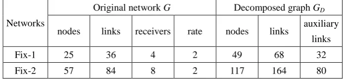
[image:12.595.172.423.490.657.2]We consider 14 test instances, four on fixed networks and 10 on randomly generated networks. The four fixed networks are 3-copy, 7-copy, 15-copy and 31-copy networks which have been used to test the performance of EAs for a number of network coding based optimization problems (Kim et al, 2007b; Xing and Qu, 2011a, 2012, 2013). Fig.9 illustrates an example of n-copy network, where Fig.9(b) is a 3-copy network constructed by cascading 3 copies of the original network in Fig.9(a). In a n-copy network, the source is the node on the top and the receivers are at the bottom. The n-copy network has n + 1 receivers to which data rate from the source is 2. We hereafter call 3-copy, 7-copy, 15-copy and 31-copy networks as Fix-1, Fix-2, Fix-3, and Fix-4 networks, respectively. The 10 random networks (Rnd-i, i = 1,…,10) are directed networks with 20 to 60 nodes. Table 1 shows the 14 instances and their parameters. To encourage scientific comparisons, all instances are provided at http://www.cs.nott.ac.uk/~rxq/benchmarks.htm. The predefined number of generations for all algorithms tested is set to 200. All experiments were run on a Windows XP computer with Intel(R) Core(TM)2 Duo CPU E8400 3.0GHz, 2G RAM. The results are achieved by running each algorithm 50 times.
Fig.9 An example of n-copy network (a) original network (b) 3-copy Table 1 Experimental Networks and Instance Parameters
Networks
Original network G Decomposed graph GD
nodes links receivers rate nodes links auxiliary
links
Fix-1 25 36 4 2 49 68 32
[image:12.595.123.470.705.785.2]Fix-3 121 180 16 2 253 356 176
Fix-4 249 372 32 2 617 740 368
Rnd-1 20 37 5 3 54 81 43
Rnd-2 20 39 5 3 65 89 50
Rnd-3 30 60 6 3 94 146 86
Rnd-4 30 69 6 3 113 181 112
Rnd-5 40 78 9 3 124 184 106
Rnd-6 40 85 9 4 91 149 64
Rnd-7 50 101 8 3 178 246 145
Rnd-8 50 118 10 4 194 307 189
Rnd-9 60 150 11 5 239 385 235
Rnd-10 60 156 10 4 262 453 297
4.2 Deficiency of BLS and BTS encodings
Different encoding approaches could greatly affect the performance of EAs (Mitchell, 1996). The resulting search spaces may be significantly different with respect to not only the size but also the structure and connectivity of the underlying landscape. As discussed in subsection 3.2, in theory, the search space of BLS or BTS encoding may contain many infeasible solutions. The solutions are thus scattered in disconnected feasible regions in the search space. The connectivity among feasible solutions may be so weak that to find optimal solution(s) by EAs becomes extremely difficult.
[image:13.595.126.471.99.297.2]In this section, we statistically measure the proportion of infeasible solutions (PIS) over search space by randomly sampling. The number of samples is fixed at 10 000 for each instance. Table 2 shows the results of PIS over 10 000 samples. For all instances, the PIS values are more than 99%. In particular, in Fix-2,3,4 and Rand-5,7,8,9,10, the PISs of BLS and BTS are always 100%, meaning that all samples are infeasible solutions which constitute the majority of the search space. Large amount of infeasible solutions could disconnect feasible regions in the search space and dramatically increase the problem difficulty for search algorithms. Hence, the BLS and BTS encodings may not be appropriate encoding schemes for our target problem.
Table 2 Results of PIS over 10 000 Samples (%)
Networks BLS BTS Networks BLS BTS
Fix-1 99.83 99.85 Rnd-4 99.83 99.35
Fix-2 100.00 100.00 Rnd-5 100.00 100.00
Fix-3 100.00 100.00 Rnd-6 99.98 99.91
Fix-4 100.00 100.00 Rnd-7 100.00 100.00
Rnd-1 99.41 99.25 Rnd-8 100.00 100.00
Rnd-2 99.96 99.99 Rnd-9 100.00 100.00
Rnd-3 99.89 99.84 Rnd-10 100.00 100.00
4.3 Performance Measures
Mean and standard deviation (SD) of the best solutions found over 50 runs. One best solution is obtained in one run. The mean and SD are important metrics to show the overall performance of a search algorithm.
Student’s t-test (Walpole et al, 2007; Yang and Yao, 35) to compare two algorithms (e.g. A1 and A2) in terms of the fitness values of the 50 best solutions obtained. In this paper, two-tailed t-test with 98 degrees of freedom at a 0.05 level of significance is used. The t-test result can show statistically if the performance of A1 is better than, worse than, or equivalent to that of A2.
Successful ratio (SR) of finding an optimal solution in 50 runs. The successful ratio, to some extent, reflects the global exploration ability of an EA to find optimal solutions.
Evolution of the best fitness averaged over 50 runs. The plot of the evolution illustrates the convergence process of an algorithm.
Average computational time (ACT) consumed by an algorithm over 50 runs. This metric is a direct indication of the time complexity of an algorithm.
4.4 The Effectiveness of Crossover in pEA
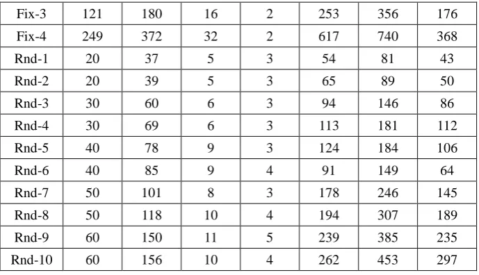
As mentioned in subsection 3.5, the single-point crossover is used in pEA. We investigate the feasibility of this operator and the impact of different settings of the crossover probability pc on the performance of pEA. Mutation and LS operator is excluded in pEA in this experiment. We set the population size pop = 20 and compare the performance of pEA with four different pc, i.e. 0.0, 0.3, 0.6, and 0.9, where pc = 0.0 means the algorithm stops after initialization since no crossover is involved. By comparing the results of different pc and those of pc = 0.0, one could see the effectiveness of the crossover.
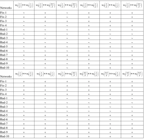
[image:14.595.99.498.631.790.2]The results of the mean and standard deviation of pEA with different pc are shown in Table 3. It can be seen that pEA with crossover performs better than pEA without crossover in each instance, indicating crossover can properly drive the evolution process. Besides, we find with larger pc the mean and SD become increasingly better. The variant of pEA with pc = 0.9 performs the best, showing that rapid exchange of genetic information over different chromosomes helps to explore different areas in the search space. However, we may also find that there remain big gaps between the best solutions obtained by pEA with only crossover and the optimal solutions in each instance. This is mainly because employing crossover only is not enough to guide pEA to escape from local optima. We need mutation to enhance local exploitation and avoid prematurity.
Table 3 Comparisons of pEA with Different Crossover Probabilities (Best Results are in Bold)
Networks
pc = 0.0 pc = 0.3 pc = 0.6 pc = 0.9
Mean SD Mean SD Mean SD Mean SD
Fix-1 2.84 0.37 1.70 0.61 1.32 0.51 1.08 0.27
Fix-2 9.58 1.45 7.64 1.43 6.78 1.35 6.16 1.23
Fix-3 22.88 0.47 20.68 1.92 19.74 2.00 17.54 1.98
Fix-4 46.94 0.42 45.32 1.89 44.72 1.79 43.20 2.26
Rnd-1 2.44 0.64 1.70 0.64 1.18 0.66 0.96 0.66
Rnd-2 0.62 0.56 0.12 0.32 0.04 0.19 0.02 0.14
Rnd-3 2.64 0.56 1.86 0.70 1.40 0.72 1.22 0.64
Rnd-4 0.72 0.45 0.38 0.49 0.22 0.41 0.10 0.30
Rnd-6 0.40 0.49 0.00 0.00 0.00 0.00 0.00 0.00
Rnd-7 3.86 1.01 3.06 0.79 2.96 1.02 2.34 0.77
Rnd-8 6.84 0.42 5.76 1.04 5.28 1.10 4.64 1.10
Rnd-9 6.00 0.00 5.42 0.67 5.14 0.63 4.98 0.58
Rnd-10 7.94 1.39 6.40 1.22 5.54 1.51 5.18 1.17
4.5 The Effectiveness of Mutation in pEA
We propose two mutation operators with pm = 1/d in section 3.6, i.e. the ordinary mutation M1 and greedy mutation M2, where d is the number of receivers. To mutate a BU, M1 deletes a random auxiliary link of the BU from GD while M2 deletes a random auxiliary link of the BU and a number of unoccupied auxiliary links from GD. The removal of the random link is to make sure that the mutated BU is different from the old one. Besides, the removal of those unoccupied links is to ensure no extra coding link will be introduced after mutation.
In the following experiment, we compare the performance of pEA with the proposed crossover and different mutations. The comparison between M1 and M2 can show whether the removal of those unoccupied auxiliary links helps to improve the performance of pEA. When comparing M1 and M2, we also study the impact of different pm, i.e. 2/d, 1/d, and 0.5/d. Let M1(pm) and M2(pm) denote the two mutations with pm, respectively. In the experiment, LS operator is excluded. We set pop = 20 and pc = 0.9.
[image:15.595.97.499.102.174.2]Table 4 shows the results of mean and standard deviation of the obtained best fitness values by pEA with different mutations and different pm. Between the two mutations, we find that pEA with M2 performs better than pEA with M1 if taking into account the results for all instances. The worst pm for M2 is 0.5/d while the best pm for M1 is 1/d. If comparing the results of M2(0.5/d) and those of M1(1/d), we see that M2(0.5/d) wins in 9 instances while M1(1/d) wins in 2 instances, indicating M2 is more effective than M1. In addition, having a look at M2 with different pm, we also find that the mean and SD become better and better with pm changing from 0.5/d to 2/d. This is because when mutating a BU, M2 makes sure that the rebuilt BU does not increase the amount of coding operations to the corresponding chromosome. On the contrary, it is possible that coding at one or more nodes of a chromosome is eliminated after M2. Hence, imposing reasonably more M2 operations to the evolving population is more likely to obtain a better optimization performance of pEA. We hereafter only use the greedy mutation as the mutation operator in our pEA.
Table 4 Results of Mean and Standard Deviation for Different Mutations and Different Mutation Probabilities (Best Results are in Bold)
Networks d 2
M1
d 1
M1
d 5 . 0
M1
d 2
M2
d 1
M2
d 5 . 0 M2
Mean SD Mean SD Mean
Mean
ean
SD Mean SD Mean SD Mean SD
Fix-1 1.00 0.00 1.00 0.00 1.00 0.00 0.04 0.19 0.14 0.35 0.26 0.44
Fix-2 4.06 0.23 4.00 0.00 4.00 0.00 1.26 0.59 1.64 0.80 1.94 0.79
Fix-3 10.52 1.05 8.50 0.54 8.44 0.57 5.72 1.22 6.04 0.92 6.68 0.84
Fix-4 29.08 1.81 24.30 0.92 23.54 0.88 17.60 1.50 18.20 1.19 18.30 1.55
Rnd-1 0.00 0.00 0.00 0.00 0.06 0.23 0.00 0.00 0.04 0.19 0.06 0.23
Rnd-2 0.00 0.00 0.00 0.00 0.00 0.00 0.00 0.00 0.00 0.00 0.00 0.00
Rnd-3 0.02 0.14 0.00 0.00 0.06 0.23 0.00 0.00 0.04 0.19 0.02 0.14
Rnd-4 0.00 0.00 0.00 0.00 0.00 0.00 0.00 0.00 0.00 0.00 0.00 0.00
Rnd-5 1.88 0.43 1.40 0.53 1.50 0.61 0.00 0.00 0.02 0.14 0.12 0.32
[image:15.595.54.546.606.798.2]Rnd-7 1.06 0.23 1.02 0.14 1.10 0.30 0.12 0.32 0.34 0.47 0.56 0.50
Rnd-8 2.10 0.30 2.16 0.37 2.34 0.51 0.02 0.14 0.04 0.19 0.30 0.46
Rnd-9 2.46 0.57 2.06 0.46 2.36 0.66 0.80 0.40 0.86 0.35 0.94 0.23
Rnd-10 1.92 0.48 1.62 0.49 1.76 0.59 0.00 0.00 0.00 0.00 0.06 0.23
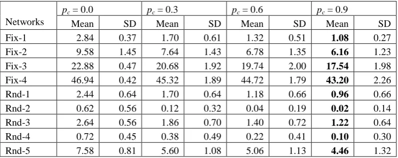
[image:16.595.56.542.308.778.2]To further support our findings, we compare different mutations with different pm by using Student’s t-test (see subsection 4.3), where results are given in Table 5. The result of comparison between A1↔A2 is shown as “+”, “–”, or “~” when A1 is significantly better than, significantly worse than, or statistically equivalent to A2, respectively. The table shows that M2 is significantly better than M1 in 9 instances and statistically equivalent to M1 in the remaining instances, which undoubtedly reflects the superiority of M2 over M1. Moreover, M2 with a larger pm performs better than M2 with a smaller pm. However, their performances do not differ too much. For example, between M2(2/d) and M2(1/d), the former only wins 2 instances.
Table 5 t-Test Results for Different Mutations and Different Mutation Probabilities
Networks
d 2 2
M
d 1 2 M d 2 2
M
d 5 . 0 2 M d 1 2
M
d 5 . 0 2 M d 2 2
M
d 2 1 M d 2 2
M
d 1 1 M d 2 2
M
d 5 . 0 1 M
Fix-1
Fix-2
Fix-3
Fix-4
Rnd-1
Rnd-2
Rnd-3
Rnd-4
Rnd-5
Rnd-6
Rnd-7
Rnd-8
Rnd-9
Rnd-10
Networks
d 1 2
M
d 2 1 M d 1 2
M
d 1 1 M d 1 2
M
d 5 . 0 1 M d 5 . 0 2
M
d 2 1 M d 5 . 0 2
M
d 1 1 M d 5 . 0 2
M
d 5 . 0 1 M
Fix-1
Fix-2
Fix-3
Fix-4
Rnd-1
Rnd-2
Rnd-3
Rnd-4
Rnd-5
Rnd-6
Rnd-7
Rnd-8
Rnd-9
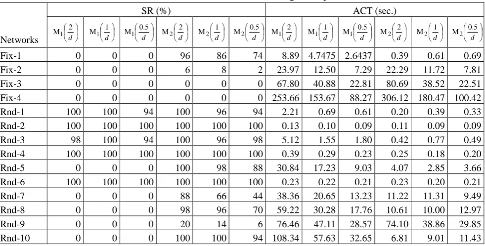
The results of the successful ratio and average computational time are collected in Table 6. For the successful ratio, the results match to our findings from Table 4, where M2 is better than M1 and a larger pm results into a better performance of M2. For the average computational time, we find that the computational complexity of mutation is higher than that of evaluation.
Table 6 Results of Successful Ratio and Average Computational Time
Networks
SR (%) ACT (sec.)
d 2
M1
d 1
M1
d 5 . 0
M1
d 2
M2
d 1
M2
d 5 . 0
M2
d 2
M1
d 1
M1
d 5 . 0
M1
d 2
M2
d 1
M2
d 5 . 0 M2
Fix-1 0 0 0 96 86 74 8.89 4.7475 2.6437 0.39 0.61 0.69
Fix-2 0 0 0 6 8 2 23.97 12.50 7.29 22.29 11.72 7.81
Fix-3 0 0 0 0 0 0 67.80 40.88 22.81 80.69 38.52 22.51
Fix-4 0 0 0 0 0 0 253.66 153.67 88.27 306.12 180.47 100.42
Rnd-1 100 100 94 100 96 94 2.21 0.69 0.61 0.20 0.39 0.33
Rnd-2 100 100 100 100 100 100 0.13 0.10 0.09 0.11 0.09 0.09
Rnd-3 98 100 94 100 96 98 5.12 1.55 1.80 0.42 0.77 0.49
Rnd-4 100 100 100 100 100 100 0.39 0.29 0.23 0.25 0.18 0.20
Rnd-5 0 0 0 100 98 88 30.84 17.23 9.03 4.07 2.85 3.66
Rnd-6 100 100 100 100 100 100 0.23 0.22 0.21 0.23 0.20 0.21
Rnd-7 0 0 0 88 66 44 38.36 20.65 13.23 11.22 11.31 9.49
Rnd-8 0 0 0 98 96 70 59.22 30.28 17.76 10.61 10.00 12.97
Rnd-9 0 0 0 20 14 6 76.46 47.11 28.57 74.10 38.86 29.85
Rnd-10 0 0 0 100 100 94 108.34 57.63 32.65 6.81 9.01 11.43
In general, fitness evaluation is assumed to be the most time-consuming operation compared with other operations such as selection, crossover and mutation for highly complex optimization problems. However, the above assumption is no longer held in pEA (without the LS operator) where mutation takes a comparable larger computation time over the fitness evaluation. In mutations (i.e. M1 and M2), computation is spent on two steps, i.e. the removal of some auxiliary links from the decomposed graph GD and the reconstruction of a new BU. The max-flow algorithm in (Goldberg, 1985) is used, leading to a time complexity of O(|VD|2·|ED|1/2), where |VD| and |ED| are the number of nodes and links in GD, respectively. Compared with the reconstruction of the BU, the removal of auxiliary links consumes very limited computation and can be ignored. Hence, to mutate a chromosome (no matter M1 or M2), we require a complexity of OM, where OM = O(pm·d·|VD|2·|ED|1/2). In contrast, to evaluate a chromosome, we only need to obtain the NCM subgraph GNCM of this chromosome and check how many outgoing auxiliary nodes perform coding in GNCM. As mentioned in section 3.3, each GNCM consists of d BUs, each of which contains R paths, e.g. pi(s,tk) is the i-th path of the k-th BU. Let Lik be the string length of pi(s,tk) in the chromosome. To obtain a GNCM from the corresponding chromosome, the amount of computation involved is ∑i∑kLik, where Lik < |VD|. We assume there are Y outgoing auxiliary nodes in GD where Y < |VD| since at least the source and receivers are not decomposed. To check the status of all outgoing auxiliary nodes in GNCM, the amount of computation involved is Y. Therefore, to evaluate a chromosome requires a complexity of OE < O(|VD|
2
) < OM.
operations during the evaluation, we should look at those instances where the successful ratios for different mutation rates are all 0%. In these instances the amount of mutation operations for different pm is proportional and we only need to check if the computational time is also proportional. Taking instance Fix-3 as an example, theoretically, the ratio of the amount of mutations during the evolution for M2(2/d), M2(1/d) and M2(0.5/d) is 4:2:1. In practice, the ratio of the average computational time of M2(2/d), M2(1/d) and M2(0.5/d) are calculated as 3.58:1.71:1.00 which is similar to the theoretical ratio.
4.6 Comparisons of Different Encoding Approaches
In this section, we show the superiority of the path-oriented encoding over other existing encoding approaches by comparing the performance of three EAs, i.e. pEA, GA with BLS encoding (BLSGA) and GA with BTS encoding (BTSGA). For the BLS and BTS encoding approaches please see (Kim et al, 2007b) and section 3.2 for details. Note that an all-one chromosome is inserted into the initial population of BLSGA and BTSGA to make sure they begin with at least one feasible solution; otherwise, the two GAs may never converge since no feasible solution may be obtained during the search (Kim et al, 2007b). This has showed to be an effective method in previous work (Kim et al, 2007a, 2007b; Xing and Qu, 2011a, 2011b, 2012, 2013).
The comparison is based on a standard GA framework, where genetic operators in each EA include selection, crossover and mutation. The population size and the tournament size are set to 20 and 2 for each algorithm, respectively. In pEA, we use the greedy mutation and set pc = 0.9 and pm = 1/d. We adopt the best parameter settings for BLSGA and BTSGA in (Kim et al, 2007b). In BLSGA, pc = 0.8 and pm = 0.006. In BTSGA, pc = 0.8 and pm = 0.012. Besides, BLSGA and BTSGA use the uniform crossover with a mixing ratio of 0.5 and a simple mutation where each bit of a chromosome is flipped at pm.
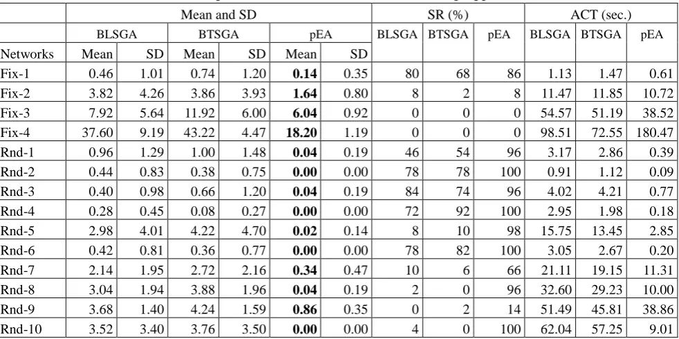
[image:18.595.54.545.534.779.2]The performance comparisons of EAs with different encodings are shown in Table 7. Besides, the t-test results are provided in Table 8. Undoubtedly, pEA achieves better optimization results and consumes less ACT than BLSGA and BTSGA in almost all instances.
Table 7 Comparisons of GA with Different Encoding Approaches
Mean and SD SR (%) ACT (sec.)
BLSGA BTSGA pEA BLSGA BTSGA pEA BLSGA BTSGA pEA
Networks Mean SD Mean SD Mean SD
Fix-1 0.46 1.01 0.74 1.20 0.14 0.35 80 68 86 1.13 1.47 0.61
Fix-2 3.82 4.26 3.86 3.93 1.64 0.80 8 2 8 11.47 11.85 10.72
Fix-3 7.92 5.64 11.92 6.00 6.04 0.92 0 0 0 54.57 51.19 38.52
Fix-4 37.60 9.19 43.22 4.47 18.20 1.19 0 0 0 98.51 72.55 180.47
Rnd-1 0.96 1.29 1.00 1.48 0.04 0.19 46 54 96 3.17 2.86 0.39
Rnd-2 0.44 0.83 0.38 0.75 0.00 0.00 78 78 100 0.91 1.12 0.09
Rnd-3 0.40 0.98 0.66 1.20 0.04 0.19 84 74 96 4.02 4.21 0.77
Rnd-4 0.28 0.45 0.08 0.27 0.00 0.00 72 92 100 2.95 1.98 0.18
Rnd-5 2.98 4.01 4.22 4.70 0.02 0.14 8 10 98 15.75 13.45 2.85
Rnd-6 0.42 0.81 0.36 0.77 0.00 0.00 78 82 100 3.05 2.67 0.20
Rnd-7 2.14 1.95 2.72 2.16 0.34 0.47 10 6 66 21.11 19.15 11.31
Rnd-8 3.04 1.94 3.88 1.96 0.04 0.19 2 0 96 32.60 29.23 10.00
Rnd-9 3.68 1.40 4.24 1.59 0.86 0.35 0 2 14 51.49 45.81 38.86
Table 8 t-Test Results for Different GAs
Networks pEABLSGA pEABTSGA Networks pEABLSGA pEABTSGA
Fix-1 Rnd-4
Fix-2 Rnd-5
Fix-3 Rnd-6
Fix-4 Rnd-7
Rnd-1 Rnd-8
Rnd-2 Rnd-9
Rnd-3 Rnd-10
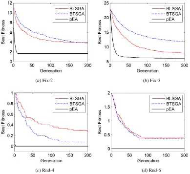
To show the convergence of the three EAs, we plot the evolution of the best fitness in each generation, averaged over 50 runs for two fixed and four random instances, as shown in Fig.10. First, we can see that pEA always obtains better initial solutions than BLSGA and BTSGA. For example, in Fig.10(a), at the beginning of the evolution, the average best fitness for pEA is around 7 while those of BLSGA and BTSGA are both 11. Moreover, we find that pEA converges very fast especially in the early generations. To find a good solution, pEA needs much less generations than BLSGA and BTSGA. This is an outstanding advantage of pEA especially in real-time and dynamic applications, where a decent solution must be found within a very short time.
(a) Fix-2 (b) Fix-3
(e) Rnd-8 (f) Rnd-10
Fig.10 Best fitness vs. generation for six instances
Based on the analysis above, we conclude that the path-oriented encoding is more efficient than the BLS and BTS encodings in terms of global optimization, convergence, and computational time.
4.7 The Effectiveness of the LS Operator
As discussed in subsection 3.7, a LS operator is applied to a randomly chosen chromosome at each generation to improve the solution quality. To verify the effectiveness of this operator, we randomly construct five chromosomes for each instance by using the initialization method in section 3.4. We apply the LS operator on each chromosome and compare the fitness values of the chromosome before and after implementing the LS operator, i.e. ФBEF and ФAFT. Let X and X denote the chromosome before and after the LS, and EA(X) and EA(X) be the set of auxiliary links owned by X and X, respectively. We define the structural difference coefficient (SDC) ρ between X and X according to the Marczewski-Steinhaus concept of distance (Marczewski and Steinhaus, 1958), as follows:
% 100 |
) ' ( ) ( |
| ) ' ( ) ( | | ) ' ( ) (
|
X X
X X
X X
A A
A A
A A
E E
E E
E E
(3)
The value of SDC is between 0.0 and 1.0, which tells us to what degree X and X are different, showing the effect of LS operator on the structure change of solutions. A larger SDC indicates a severer structural change caused by the LS operator.
Table 9 Results of the LS Operator
Networks
Solution 1 Solution 2 Solution 3 Solution 4 Solution 5
ΦBEF ΦAFT ρ (%) ΦBEF ΦAFT ρ (%) ΦBEF ΦAFT ρ (%) ΦBEF ΦAFT ρ (%) ΦBEF ΦAFT ρ (%)
Fix-1 3 0 54.5 4 0 20.0 3 0 30.0 5 0 36.3 6 0 50.0
Fix-2 12 0 51.7 18 0 53.1 13 0 54.8 16 0 56.2 14 0 53.3
Fix-3 30 0 54.5 35 0 56.3 27 0 54.5 29 0 55.2 40 0 52.8
Fix-4 47 0 53.4 69 0 53.8 60 0 53.9 71 0 54.9 70 0 57.3
Rnd-1 4 2 36.0 5 3 17.3 2 0 30.0 7 3 26.9 6 1 38.4
Rnd-2 2 0 8.33 3 2 18.5 5 3 7.41 4 2 11.5 3 1 33.3
Rnd-3 3 0 38.8 3 0 19.3 5 1 34.1 7 0 45.2 6 0 50.0
Rnd-4 4 1 25.7 5 2 25.6 4 0 22.8 1 0 13.7 2 1 42.1
Rnd-5 12 7 20.0 9 3 17.8 11 3 21.8 8 4 23.6 10 2 39.6
[image:20.595.63.537.614.791.2]Rnd-7 8 4 20.0 6 2 28.3 4 1 10.2 9 3 13.5 6 5 8.33
Rnd-8 8 5 10.5 12 7 15.8 11 3 29.8 15 8 20.4 14 5 22.0
Rnd-9 13 7 15.7 18 5 21.7 8 4 12.3 14 4 19.7 12 7 15.9
Rnd-10 12 3 30.8 15 5 24.5 8 5 8.89 9 5 10.9 7 3 31.1
The experimental results of ФBEF, ФAFT and ρ are shown in Table 9. First, it is seen that ФEND is smaller than ФSTART especially for instances Fix-3,4, showing that the LS operator can improve the quality of chromosomes. Meanwhile, regarding the values of ρ in all instances, 32 chromosomes (45% of the 70 chromosomes) are at least 30% different on the structure, meaning the LS operator may also help to introduce extra diversity to the population.
4.8 Overall performance Evaluation
This section evaluates the overall performance of pEA by comparing it with six state-of-the-art algorithms in the literature. The following explains the algorithms for comparison.
GA1: BLS encoding based GA (Kim et al, 2007b). Different from BLSGA used in section 4.6, GA1 employs a greedy sweep operator after the evolution to further improve the quality of the best solution found by flipping each of the remaining 1’s to 0 if it does not result into an infeasible solution.
GA2: BTS encoding based GA (Kim et al, 2007b). The same greedy sweep operator is applied at the end of evolution as in GA1.
QEA1: Quantum-inspired evolutionary algorithm (QEA) (Xing et al, 2010). QEA maintains a population of quantum-bit chromosomes. Each chromosome is a probabilistic distribution model over the solution space. Each sampling on a chromosome results into a solution. Rotation angle step (RAS) and quantum mutation probability (QMP) are used to update each chromosome. QEA1 is based on the BLS encoding. For each chromosome, the RAS value is randomly generated and the QMP value is set according to the current fitness of the chromosome.
QEA2: Another QEA proposed by Ji and Xing (2011). The main difference between QEA2 and QEA1 is that in QEA2 the RAS and QMP values of a chromosome are adjusted according to the current and previous fitness values of the chromosome.
PBIL: Population based incremental learning algorithm (Xing and Qu, 2011a). BLS encoding is used. PBIL maintains a real-valued probability vector (PV) which, when sampled, produces promising solutions with higher probabilities. At each generation, the statistic information of high quality samples is used to update the PV. A restart scheme is introduced to help PBIL to escape from local optima.
cGA: Compact genetic algorithm (Xing and Qu, 2012). Similar to PBIL, cGA also maintains a PV. However, the PV in cGA is only sampled once at each generation. The new sample is compared with the best-so-far sample and between the two the winner is used to update the PV. Based on BLS encoding, cGA is featured by a restart scheme and a local search operator.
pEA1: the path-oriented encoding EA. Note that LS operator is excluded. The performance of pEA1 will demonstrate the pure evolutionary search ability of the proposed algorithm.
(Xing et al, 2010; Ji and Xing, 2011; Xing and Qu, 2011a, 2012). For pEA\LS and pEA, we set pc = 0.9 and pm = 1/d, where d is the number of receivers.
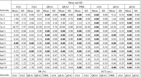
The comparison results are collected in Table 10, where the best results in mean are in bold. First, we analyze the data in Mean and SR for each algorithm. It can be seen that pEA2 always performs the best in each instance while cGA is the second best. The third best algorithm is PBIL. Compared with QEA1 and QEA2, PBIL performs better in 6 instances (see Fix-2,3 and Rnd-5,7,9,10) and worse in 2 instances (see Fix-4 and Rnd-8). The comparison of pEA1 and pEA2 illustrates that LS operator help to improve the overall performance of the proposed algorithm. In some cases the improvement is substantial, e.g. the mean and SR in instances Fix-2,3,4. When comparing pEA1 with the existing algorithms, we can see that in fix networks, pEA1 has similar performance with GA1. In random networks, pEA1 gains similar performance with PBIL except for instances Rnd-8,9 and illustrates better performance than GAs and QEAs in most instances.
[image:22.595.52.549.523.797.2]Next, we compare the ACT of the algorithms. Before analyzing the data, we divide the 14 instances into two groups according to their PIS values (see subsection 4.2). Those with a PIS value less than 100% belong to the first group (called easy instances) while the rest belong to the second group (called hard instances). Easy instances includes Fix-1 and Rnd-1,2,3,4,6 while hard instances are Fix-2,3,4 and Rnd-5,7,8,9,10. Regarding easy instances, one can find that more than half of the state-of-the-art algorithms (GA1, GA2, QEA1, QEA2, PBIL, and cGA) can find an optimal solution with a successful ratio of 100%. As for hard instances, most of the state-of-the-art algorithms have a lower successful ratio than 100%. In easy instances, most of algorithms can obtain an optimal solution within a short time (e.g. less than 1 second). However, in each hard instance, the ACT spent by each algorithm differs significantly. In easy instances, QEA1, QEA2, PBIL, cGA, pEA1 and pEA2 all consume similar ACT (i.e. less than 1 second) while GA1 and GA2 are the two worst. In hard instances, pEA2 and cGA are the two fastest algorithms. Besides, the former costs significantly less time than the latter in instances Fix-3,4 and Rnd-5,8,9,10. pEA1 is the third fastest algorithm. The difference between pEA1 and pEA2 also indicates the effectiveness of LS in reducing the computational time.
Table 10 Comparisons of Different Algorithms
Networks
Mean and SD
GA1 GA2 QEA1 QEA2 PBIL cGA pEA1 pEA2
Mean SD Mean SD Mean SD Mean SD Mean SD Mean SD Mean SD Mean SD
Fix-1 0.36 0.74 0.08 0.27 0.00 0.00 0.00 0.00 0.00 0.00 0.00 0.00 0.14 0.35 0.00 0.00
Fix-2 1.96 1.92 0.68 0.84 0.18 0.62 0.48 0.70 0.00 0.00 0.00 0.00 1.64 0.80 0.00 0.00
Fix-3 7.48 5.12 3.66 2.13 3.10 4.18 5.80 1.62 2.14 4.31 0.00 0.00 6.04 0.92 0.00 0.00
Fix-4 28.75 7.97 18.66 22.58 19.10 5.76 20.00 0.00 28.90 10.30 0.00 0.00 18.20 1.19 0.00 0.00
Rnd-1 0.52 0.88 0.44 0.50 0.00 0.00 0.00 0.00 0.00 0.00 0.00 0.00 0.04 0.19 0.00 0.00
Rnd-2 0.26 0.66 0.02 0.14 0.00 0.00 0.00 0.00 0.00 0.00 0.00 0.00 0.00 0.00 0.00 0.00
Rnd-3 0.44 0.83 0.02 0.14 0.00 0.00 0.00 0.00 0.00 0.00 0.00 0.00 0.04 0.19 0.00 0.00
Rnd-4 0.00 0.00 0.00 0.00 0.00 0.00 0.00 0.00 0.00 0.00 0.00 0.00 0.00 0.00 0.00 0.00
Rnd-5 2.78 2.71 1.16 0.61 0.46 0.50 0.48 0.54 0.04 0.28 0.04 0.19 0.02 0.14 0.00 0.00
Rnd-6 0.22 0.41 0.00 0.00 0.00 0.00 0.00 0.00 0.00 0.00 0.00 0.00 0.00 0.00 0.00 0.00
Rnd-7 1.58 0.92 1.36 0.66 0.66 0.47 0.58 0.53 0.38 0.60 0.22 0.41 0.34 0.47 0.00 0.00
Rnd-8 2.52 1.44 2.28 0.94 0.98 0.82 0.48 0.61 0.60 1.56 0.24 0.43 0.04 0.19 0.00 0.00
Rnd-9 2.82 1.22 2.34 1.34 1.64 0.98 1.94 1.16 0.06 0.23 0.04 0.19 0.86 0.35 0.00 0.00
Rnd-10 3.26 2.68 1.38 0.69 0.66 0.68 0.42 0.64 0.00 0.00 0.08 0.27 0.00 0.00 0.00 0.00
Networks
SR (%) ACT (sec.)
Fix-1 80 92 100 100 100 100 86 100 0.99 1.61 0.24 0.21 0.10 0.02 0.61 0.09
Fix-2 14 52 88 62 100 100 8 100 12.42 11.98 8.54 10.41 2.20 0.15 10.72 0.33
Fix-3 0 4 26 0 58 100 0 100 55.85 49.27 89.88 91.61 66.14 2.09 38.52 1.57
Fix-4 0 0 0 0 0 100 0 100 232.92 200.73 728.13 750.70 543.64 29.55 180.47 20.79
Rnd-1 62 56 100 100 100 100 96 100 2.95 3.30 0.73 0.50 0.29 0.23 0.39 0.16
Rnd-2 86 98 100 100 100 100 100 100 1.14 1.33 0.37 0.40 0.13 0.02 0.09 0.11
Rnd-3 76 98 100 100 100 100 96 100 5.13 5.07 0.68 0.75 0.23 0.06 0.77 0.27
Rnd-4 100 100 100 100 100 100 100 100 3.19 3.13 0.57 0.81 0.26 0.16 0.18 0.23
Rnd-5 4 10 54 54 98 96 98 100 16.57 14.52 13.82 14.38 6.09 3.14 2.85 0.63
Rnd-6 78 100 100 100 100 100 100 100 3.54 3.34 0.72 0.84 0.17 0.03 0.20 0.23
Rnd-7 8 8 34 44 68 78 66 100 24.13 20.78 24.35 22.52 24.29 6.83 11.31 2.10
Rnd-8 2 0 30 58 82 76 96 100 38.37 30.89 38.04 31.47 27.43 20.11 10.00 0.95
Rnd-9 4 8 14 10 94 96 14 100 62.46 50.73 73.73 73.94 47.29 16.40 38.86 1.93
Rnd-10 4 6 46 64 100 92 100 100 71.25 55.46 64.12 52.39 31.81 17.42 9.01 1.15
[image:23.595.68.531.402.607.2]Regarding the overall performance in Table 10, we see that pEA2 is the best among the eight algorithms. Besides, pEA1 has similar performance with GA1 in fix networks and PBIL in random networks, respectively. Meanwhile, the LS operator has a positive impact on improving the overall performance of the proposed algorithm. To further support the finding, we show the t-test results comparing pEA2 and pEA1 with the others in Table 11.
Table 11 t-Test Results for Comparing Different Algorithms
Networks Fix-1 Fix-2 Fix-3 Fix-4 Rnd-1 Rnd-2 Rnd-3 Rnd-4 Rnd-5 Rnd-6 Rnd-7 Rnd-8 Rnd-9 Rnd-10
pEA2GA1
pEA2GA2
pEA2QEA1
PEA2QEA2
pEA2PBIL
pEA2cGA
pEA2pEA1 + +
pEA1GA1 + + + +
pEA1GA2 + + + +
pEA1QEA1 + + + +
pEA1QEA2 + + + +
pEA1PBIL +
pEA1cGA + +
Note: The result of comparison between Algorithm1↔Algorithm2 is shown as “+”, “–”, or “~” when the former is significantly
better than, significantly worse than, or statistically equivalent to the latter, respectively.
5. Conclusions
ordinary mutation. Besides, a problem-specific local search operator is also developed to improve the solution quality. The simulation results show that the proposed pEA outperforms six existing state-of-the-art algorithms regarding the best solutions obtained and the computational time consumed, due to the new path-oriented encoding and the associated operators designed accordingly.
References
Ahlswede R, Cai N, Li S Y R, and Yeung R W (2000). Network information flow. IEEE Transactions on Information
Theory46(4): 1204-1216.
Ahn C W and Ramakrishna R S (2002). A genetic algorithm for shortest path routing problem and the sizing of
populations. IEEE Transactions on Evolutionary Computation6(6): 566-579.
Ahn C W (2011). Fast and adaptive evolutionary algorithm for minimum-cost multicast with network coding.
Electronics Letters 47(12): 700-701.
Cheng H and Yang S (2008). A genetic-inspired joint multicast routing and channel assignment algorithm in wireless
mesh networks. In: Proceedings of the 2008 UK Workshop on Computational Intelligence, pp. 159-164.
Cheng H and Yang S (2010a). Multi-population genetic algorithms with immigrants scheme for dynamic shortest path
routing problems in mobile Ad Hoc networks. In: Proceedings of EvoApplications 2010, pp. 562-571.
Cheng H and Yang S (2010b). Genetic algorithms with immigrants schemes for dynamic multicast problems in mobile
Ad Hoc networks. Engineering Applications of Artificial Intelligence23(5): 806-819.
Fragouli C, Boudec J Y L and Widmer J (2006). Network coding: an instant primer. Computer Communications Review
36(1): 63-68.
Fragouli C and Soljanin E (2006). Information flow decomposition for network coding. IEEE Transactions on
Information Theory52(3): 829-848.
Goldberg A V (1985). A new max-flow algorithm. MIT Technical Report MIT/LCS/TM-291, Laboratory for Computer
Science, MIT.
Ji Y and Xing H (2011). A memory-storable quantum-inspired evolutionary algorithm for network coding resource
minimization. In: Kita E. (Ed.), Evolutionary Algorithm. InTech, pp.363-380.
Kim M, Ahn C W, Médard M and Effros M (2006). On minimizing network coding resources: An evolutionary
approach. In: Proceedings of Second Workshop on Network Coding, Theory, and Applications (NetCod2006),
Boston.
Kim M, Médard M, Aggarwal V, O’Reilly U M, Kim W, Ahn C W and Effros M (2007a). Evolutionary approaches to
minimizing network coding resources. In: Proceedings of 26th IEEE International Conference on Computer
Communications (INFOCOM2007), Anchorage, pp. 1991-1999.
Kim M, Aggarwal V, Reilly V O, Médard M and Kim W (2007b). Genetic representations for evolutionary
minimization of network coding resources. In: Proceedings of EvoWorkshops 2007, LNCS 4448, Valencia, pp 21-31.
Langberg M, Sprintson A and Bruck J (2006). The encoding complexity of network coding. IEEE Transactions on
Information Theory52(6): 2386-2397.
Li S Y R, Yeung R W and Cai N (2003). Linear network coding. IEEE Transactions on Information Theory 49(2):
371-381.
Luong H N, Nguyen H T T and Ahn C W (2012). Entropy-based efficiency enhancement techniques for evolutionary
algorithms. Information Sciences188: 100-120.
Marczewski E and Steinhaus H (1958). On a certain distance of sets and the corresponding distance of functions.
Colloquium Mathematicum 6.
Miller C K (1998). Multicast networking and applications. Pearson Education.