Redistribution over the Lifetime in the
Irish Tax-Benefit System: An Application of
a Prototype Dynamic Microsimulation
Model for Ireland
CATHAL O’DONOGHUE*
National University of Ireland, Galway and London School of Economics
Abstract: This paper examines the distribution of lifetime income in Ireland. To do this a new prototype dynamic microsimulation model for Ireland is used to generate lifetime income streams. Aggregating over the lifetime we can assess the distribution of lifetime income and the degree of redistribution in the tax-benefit system. In addition to the effect of taxes and benefits, we decompose lifetime income into its components and examine the impact of different life-cycle patterns.
I INTRODUCTION
T
he distribution of current income and the redistributive effect of the tax-benefit system at a point in time have been extensively studied in Ireland. Typically, the accounting period, the period over which the redistribution is measured, has been relatively short (i.e. redistribution over a week or a year).191
Paper presented at the Fifteenth Annual Conference of the Irish Economic Association.
Examples include Callan and Nolan (1990, 1999). In this paper, we measure redistribution in the Irish tax-benefit system using a lifetime accounting period. The purpose of this paper is twofold. In addition to analysing the degree of redistribution over the lifetime, the paper also describes a new analytical tool designed for analysing public policy in Ireland, a dynamic microsimulation model.
The primary reasons for studying lifetime income is that income measures that cover short periods depend too much on chance. Layard (1977) argues that using short accounting periods exaggerates the basic inequality of incomes and the amount of redistribution. Short accounting periods will tend to increase the degree of income inequality measured within a population because of the nature of short-term income volatility, life-cycle effects and different career trajectories. For example, an individual, who becomes short-term unemployed from high paid employment, will be classified as poor during the period of unemployment. However over their lifetime, they may be classified as rich. Turning to life-cycle effects, pensioners will tend to be lower down the income distribution, but yet during their working lives, may have been higher up the distribution. Nelissen (1998) has highlighted the importance of career trajectories on lifetime income. Individuals who invest more in education may have lower income than those with lower education attainments earlier in their lifetimes and so be lower in the annual income distribution. However, they will tend to have higher income trajectories over their careers and as a result they will eventually pass out the lower educated in the income distribution and spend more years higher up the annual income distribution.
Empirically, panel studies have shown that there is considerable income mobility over time. For example Jarvis and Jenkins (1998) found that in Britain only 37 per cent of the poorest decile group were still in the bottom decile after four years. Björklund and Palme (1997) found in a study of dispos-able incomes 1974-1991 in Sweden, that lifetime income dispersion was 30-60 per cent of that of total income for the population over the period. Nelissen (1998) argues that the percentage of transitory income over the lifetime had increased over time due to greater career mobility. Lifetime income more fully explains an individual’s long-term potential standard of living. However, it must be noted that shorter accounting periods may be more appropriate as a measure of welfare when short-term concerns are more important especially when considering the very poor who may be credit constrained.
losers at other times. For example, Callan and Nolan (1990 and 1999), using short accounting periods, found that taxes and benefits had a significant redistributive effect that became more important over time. However, over the lifetime, the redistributive effect of taxes and benefits may be less strong. Most pensioners receive contributory benefits where benefit receipt represents a return on contributions made during the lifetime rather than as a pure distribution from rich to poor. Seniority rules will result in those with more experience earning more and so, because of the progressive nature of the income tax system, they will tend to pay a higher average tax rate during periods of their lifetime when in receipt of higher earnings.
In this paper we focus on redistribution in the Irish tax-benefit system. The system is in many respects typical of the Anglo-Liberal style of welfare state, with relatively insignificant social insurance systems, where means testing and progressive income taxes are relatively more important than in other countries. There are a number of important differences between the UK and Irish tax-benefit systems. First, means testing tends to be more import-ant. Unlike public pensions in the UK, the Irish system generally has no earnings related components, with flat rate benefits being the norm. Having a larger self-employed population, the coverage of social insurance also tends to be lower. Structurally, means tested benefits are designed differently to the UK. Although Ireland uses a set of categorical instruments for different con-tingencies, with different means tests and eligibility conditions, they together however cover the same set of contingencies as the single universal means tested benefit, income support in the UK.1 This reflects the incremental
expansion in coverage of social benefits since the foundation of the state, largely having no sweeping reforms as in the case of the Beveridgeand Fowler reforms in the UK. Housing Benefits are less important, but however are now growing in importance due to the recent growth in housing costs. Income taxes differ from the UK in that couples can optionally have their income taxed jointly.2
This paper is designed as follows. Section II describes briefly the principle methodology used in this paper, dynamic microsimulation. Section III discusses some measurement issues. The results are presented in Section IV. First, some initial results of the lifetime incidence of the tax-benefit system. We then investigate the distribution of lifetime income in Ireland. We also compare the redistributive effect of the tax-benefit system over the lifetime with that over a shorter accounting period, the year. The characteristics that
1 Income Support (IS) for pensioners has recently become the Minimum Income Guarantee, but other than a difference in the treatment of capital and benefit value, the rules are the same as for Income Support.
influence lifetime income and redistribution are then examined. Section V concludes.
II METHODOLOGY
Dynamic Microsimulation
A number of studies have examined lifetime redistribution in tax-benefit systems. One method used has been to take stylised individuals/households and to simulate given their life histories, the life-course impact of tax-benefits. Examples include “money’s worth” studies in the USA, which look at the return to state pension contributions over the lifetime. Hughes (1985) calculated rates of return in the Irish public pension system using stylised individuals, while Evans and Falkingham (1997) look at the ability of different national pension systems to provide minimum incomes in retirement for a range of different stylised life histories.
Although useful for illustration purposes, utilising stylised households and individuals however, has a number of drawbacks. Even if a wide range of stylised individuals are used, these typically only represent a small proportion of the heterogeneity of a population. In moving from a static single year analysis to life-course patterns, heterogeneity will increase as there are more variable factors and hence, stylised households will be even less repre-sentative. In order to consider life-course influences on tax-benefit systems incorporating the heterogeneity represented in the population, micro panel data is necessary. It is rare however that data exists with such a long-time horizon. Even long running household panel datasets such as the Panel Survey of Income Dynamicsin the USA and the German Socio-Economic Panelhave only 20-30 years of information. A notable exception is Björklund (1993) who used a dataset containing thirty-nine years of Swedish income data taken from register information to look at lifetime versus annual income distribution. In the absence of long running panel data, other methods have to be considered. For example, Attanasio and Banks (1998) have pooled multiple cross-sectional datasets to form pseudo-cohort to look at household savings behaviour over the life-cycle.
field has expanded as computing costs decrease and as the availability of micro-data increased. So far about 30 dynamic microsimulation models have been constructed internationally (See O’Donoghue (2001) for a survey), with approximately 10 models in active use at present.
Microsimulation models incorporate behaviour in a less comprehensive manner, than other models such as overlapping generations models (OGM) that have production sectors and models of sectoral interactions. OGM’s too can examine similar inter-temporal public finance issues as dynamic microsimulation models and furthermore can take into consideration, general equilibrium effects of public policy. However, OGM’s lack the detail of microsimulation models and so are less able to incorporate the rules of tax-benefit systems.
The limited behavioural processes included in dynamic microsimulation models depend strongly on the micro-behavioural econometric studies and household datasets on which they are based. At present there exist many knowledge gaps about the micro-economic behaviour of individuals and families both internationally and in Ireland. Internationally, the Panel on Retirement Income Modelling (Citro and Hanushek, 1997) in the USA highlights for example, that the life-cycle model of savings and consumption does not adequately explain long-run changes in personal savings behaviour. Also life-course labour supply and retirement behaviour is not well understood. In Ireland many gaps exist such as the economic determinants of demographic behaviour, empirical models of savings and wealth accumulation behaviour or earnings mobility.
The absence of good datasets also limits the development of the field. In most countries of Europe at present, only 4 waves of the European Community Household Panel are available, limiting the quantification of dynamic behaviour. Such short panel datasets will also be less able to disentangle the impact of age, cohort and period effects. Witness the difference in the age earnings relationship when estimated on cross-section or panel data. In the former case, the relationship exhibits an inverted U, while actual cohort specific age, earnings relationships tend to rise over the entire lifetime.
Dynamic microsimulation models can be divided into two types, population and cohort models (see Harding, 1993). Both types of model simulate for individual agents, life histories of processes such as education, fertility, marriage, labour market behaviour and detailed government policies. There is a computational trade-off between simulating many cohorts and simulating many years. Historically, dynamic population models opted to simulate many cohorts over the medium term of say 20-40 years. Dynamic cohort models on the other hand opted to simulate single cohorts over an entire lifetime. However, recently, as computational costs have come down, this is less of an issue.
The two models also have been used to examine different issues. Dynamic population models project forward the characteristics of a population cross-section over a number of years into the future. They take a set of underlying assumptions about the way behaviour will change over time. As a result they produce a forecast of the population at some point in the future and so in ways they are analogous to the forecasts by medium and long-term macro models. Projecting information necessary to simulate long-term policy issues such as pensions and long-term care, they can be used to examine the effect of demographic and economic changes on existing policy and also to design alternative policy instruments (See Caldwell et al., 1999).
Dynamic cohort models on the other hand, tend to make steady state assumptions, assuming that behaviour is unchanging over time, for example behaviour as observed in the mid-1990s. They then typically take a single tax-benefit system and carry out analysis on it in a steady state. (See Harding, 1993; Falkingham and Hills, 1995 and Baldini, 1997.) They therefore represent no cohort. Focusing on just one system and utilising unchanging behaviour patterns they allow one to look at the actual forces within a particular tax-benefit system that drive lifetime redistribution results without considering potential compensating interactions.
Model Description
The model used in this paper is described in more detail in O’Donoghue (2001) and can be characterised as a dynamic steady state cohort model.3The
objective of this paper is to measure the degree of redistribution over the lifetime of the Irish Tax-Benefit system. Because a synthetic panel is generated, all aspects of life-cycle behaviour that influence the tax-benefit systems needs to be simulated.4 Labour market behaviour equations are
estimated using the 1994 Living in Ireland Survey, a 4,000 household income survey, part of the European Community Panel Survey, described in Callan et al.(1996). Transitions were estimated using recall data from 1993 and current information from 1994. In the future, access to further waves of the panel will improve the model estimates. Most demographic processes such as mortality, fertility and education are estimated using official statistics.
In order to generate the correct life-cycle distribution of age and births, the main demographic processes, education, fertility, disability, marriage and mortality are simulated. While these characteristics depend primarily on age, marital status and gender, own and parental occupation and education levels are also important determinants. Because of the recent volatility in migration flows we assume no migration in the current model. Marriage is simulated by first selecting individuals in the model to marry and then by utilising a matching algorithm, potential partners are selected from the population.
The labour market process is hierarchical. First, those who are in education or become disabled are excluded from labour market participation. Second, a decision is made whether an individual retires from the labour market. This process is influenced by whether an individual suffers long-term illness or periods of long-term unemployment late in life and membership of a private pension plan. A simulation is then carried out on the remaining group to determine whether they will enter the labour market or not.5 As long
periods out of work will reduce the chances of entering work, duration variables are included. Likewise, lack of formal childcare support and lone parenthood in Ireland will have an impact on the decision.
Even when one includes these influences on the decision to work, there is a great deal of heterogeneity and thus the model is likely to produce too much career mobility. To partially limit the effect of this, we construct the notion of those in regular and marginal employment (See Atkinson and Micklewright, 1991). Membership of a pension plan or public sector employment, together with an individual’s labour market position in the previous period and a generated measure of permanence6 is used to determine regular/marginal
employment.
If an individual is determined as being in work in a period, the model then simulates whether that individual becomes an employee or opts for self-employment. Employees have a choice between two discrete labour supply states, part-time or full-time work. The self-employed have the choice between
agricultural and non-agricultural employment. Individual’s employment deci-sions in the past have a strong bearing on their current decision.
The model incorporates in a relatively simple way the influence of the tax-benefit system on labour market behaviour. Individuals optimise behaviour based on tax-benefit outcomes when deciding to work or not, when deciding to work full-time or part-time, when deciding to become self-employed and when choosing to seek work if out of work.
It would be desirable to simulate a model of savings and consumption behaviour with wealth accumulation and investment returns. Because of data problems, we instead however, employ a simpler model where only invest-ment, property income and consumption are simulated.7 Lastly, taxes and
benefits are simulated using the EUROMOD tax-benefit model (see Immervoll and O’Donoghue, 2001), which contains detailed rules of the Irish tax-benefit system together with additional modules for social insurance benefits.
A method known as alignment is used to calibrate aggregates simulated by the model with external control totals. This allows macro-economic conditions to be incorporated exogenously in the model and thus alignment contains the forecast assumptions for the simulations.
Validation
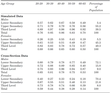
In order to validate outcomes simulated by the model, we compare life-cycle employment rates simulated by the dynamic microsimulation model with actual employment rates for the population as a whole taken from a cross-section in the 1994 Living in Ireland Survey. Table 1 describes the employment rate for individuals with different educational qualifications over the life-course. When we compare simple average employment rates, we find that employment rates are much higher for the simulated cohort for each age group than for the total population in 1994. However when one decomposes by the employment rates for different educational attainment groups, we find that employment rates are much closer.8 The upward shift in the overall
employment rates result from the compositional change in the distribution of education levels in the population. In the last column, we can see the proportion of the simulated and 1994 populations with different education levels. We see that while in 1994 only 9(8) per cent of males (females) had third level education, taking education participation rates of the mid-late
7 Blomquist, (1981) argues that as capital income is a return on savings, one should not include this in the lifetime income concept. However, as a source of income it is important to consider when comparing standards of living.
1990s we find that 39.5 (49.5) per cent of the simulated cohort have third level education. This is due to the large increase in education participation in the mid–late 1990s on which the simulated transitions are based. This is especially noticeable for older age groups and for women where this differential is greatest.9
Table 1: Employment Rate by Education Level by Age Group
Age Group 20-29 30-39 40-49 50-59 60-65 Percentage of Population
Simulated Data
Males
Lower Secondary 0.57 0.62 0.67 0.58 0.49 5.4 Upper Secondary 0.71 0.79 0.79 0.76 0.56 55.2 Third Level 0.89 0.97 0.98 0.96 0.92 39.5
Total 0.76 0.85 0.86 0.83 0.70 100
Females
Lower Secondary 0.26 0.25 0.55 0.41 0.19 5.5 Upper Secondary 0.61 0.53 0.51 0.49 0.47 45.2 Third Level 0.82 0.83 0.78 0.72 0.57 49.3
Total 0.68 0.66 0.65 0.60 0.50 100
Cross-Section Data
Males
Lower Secondary 0.60 0.79 0.78 0.77 0.49 72.1 Upper Secondary 0.72 0.88 0.89 0.85 0.40 15.8 Third Level 0.75 0.93 0.96 0.94 0.87 9.0
Total 0.65 0.81 0.78 0.75 0.53 100
Females
Lower Secondary 0.40 0.27 0.33 0.24 0.18 70.4 Upper Secondary 0.67 0.55 0.51 0.46 0.13 21.6 Third Level 0.73 0.78 0.74 0.66 0.39 8.0
Total 0.59 0.44 0.38 0.28 0.14 100
Source: Author’s Calculations and Living in Ireland Survey.
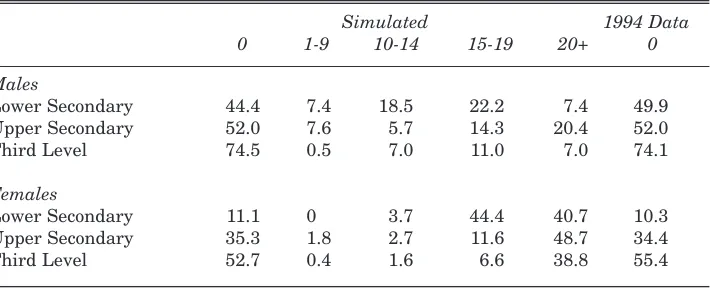
Table 1 validates the cross-sectional employment rates for different age groups. In Table 2 we consider the validity of the longitudinal simulations. Here we report the distribution of males and females by the number of years spent out of work between leaving education and entering retirement. We
notice that, like the employment rate, the distribution of years out of work is highly related to education level. Comparing the simulated cohort with the actual population, we find that the distribution is quite similar for each education level to that observed in the population. In the 1994 data, for men we consider the percentage without any employment gaps in the 55-65 age group. Older women even when accounting for different education levels have had much lower employment rates than for younger women. As a result a lower proportion of the 55-65 age group will have no years out of the labour market than for younger women. Because we assume that the behaviour of women is based on an extrapolation of current trends of younger women, it is more appropriate to compare the outputs of the model against the employment persistence of younger women. We therefore look at the proportion of women aged 30-35 who have spent no years out of work as our comparator.
Table 2: Distribution of Years Not Worked by Education Level
Simulated 1994 Data
0 1-9 10-14 15-19 20+ 0
Males
Lower Secondary 44.4 7.4 18.5 22.2 7.4 49.9 Upper Secondary 52.0 7.6 5.7 14.3 20.4 52.0
Third Level 74.5 0.5 7.0 11.0 7.0 74.1
Females
Lower Secondary 11.1 0 3.7 44.4 40.7 10.3 Upper Secondary 35.3 1.8 2.7 11.6 48.7 34.4
Third Level 52.7 0.4 1.6 6.6 38.8 55.4
Source: Author’s Calculations and Living in Ireland Survey 1994.
III MEASUREMENT ISSUES
Income Definitions
Layard (1977) describes some of the methodological issues related to the measurement of lifetime income. Because income is preferred earlier in one’s life than later (interest can be earned on accumulated wealth), it is commonplace to use a discount rate when comparing incomes at different points over time. Harding (1993) however abstracts completely from discounting, arguing that as income growth tends to follow economic growth rates and because it is reasonable to set discount rates equal to the economic growth rates, discount rate and growth rates are equal to each other and thus cancel each other out. In this paper, we make the same assumption. One problem highlighted by Falkingham and Hills (1995) is that not all income sources rise at the rate of economic growth. For example, in the UK, benefits and income tax thresholds tend to increase at the rate of prices rather than economic growth. Likewise, occupational pensions will tend to rise at a lower rate than economic growth. However, because the objective is to focus on the lifetime redistributive effect of a particular system, rather than the long-term effect of government policy, we continue with Harding’s assumption.10
An issue raised by Layard is the significance of life length. Those with the same lifetime income but different life lengths, will have different annual incomes. Annualising lifetime income by dividing by the length of life may therefore be a better measure of lifetime average welfare. Annualising will result in individuals with shorter lifetimes tending to have higher annualised lifetime income. This is because they will have proportionally less of their lifetimes in retirement. Retirement tends to be a period of lower income and therefore lower periods in retirement results in a higher proportion of life-length spent in work. Also having a longer life may result in higher transfers from the state, through pension payments for a longer period. In Caldwell et al.(1999), it was found that the longer length of life of those in higher social classes resulted in a much less progressive tax-benefit system over the lifetime.
Measuring Redistribution
In this paper the level of redistribution is calculated using measures based on the Gini coefficient:
GM=1 – 2
1
0
LM(p)dp (1)
where p is the cumulative population share and LM(p), the Lorenz Curve at point p. If Lorenz Curve A lies completely inside curve B, then it is possible to
say that population A has greater inequality than population B, with GA> GB.
However, if the Lorenz Curves cross, it is not possible to make inequality comparisons without using value judgements.
In order to measure redistribution we use the Reynolds-Smolensky index, which is defined as the difference between the Gini coefficient for market income and post-instrument income:
ΠARS= GM– GM+A= 2
1
0
[LM(p)– LM+A(p)]dp
(2)where M is market income and A are taxes and benefits.
Decomposing Income Inequality by Determinants
We would like to assess the impact, income determinants such as education, age, family structure, age at death, lifetime labour market characteristics have on total inequality of disposable and market income and thus indirectly their impact on redistribution. Decomposing inequality measures by population group is highly dependent on sample size and thus, the use of many sub-categories is often not feasible given data constraints. To get around this problem, a regression-based method has been introduced to investigate the contribution made by these factors (See Morduch and Sicular, 1998). The method starts with a decomposition of total income Y, into a regression equation as detailed in formula (3).
Y = Xβ+ ε (3)
where Xis an n ×Mvector of Mattributes described in Table 5 and ,an n ×1 vector of residuals, where nis the sample size. The next step involves splitting for each unit, i, total income into the component Yim, accounted for by each independent variable Xi:
m=1
Yi= Yim where Yim= Xim βm, for m ≤M; Yim= εi, for m = M + 1 (4) m+1
In this way, total income variability can be decomposed into its components accounted for by these independent attributes as described in (5).
n
(βm. X
im – βm. X –m
)2 m+1
i=1
I = IρmχmI .Im where Im = –––––––––––––––––––n (5)
m=1 2
(βm. Xim)
2
i=1
and the population respectively. Our redistribution measures are based on the Gini measure of inequality. However, because it is difficult to decompose the Gini index, an alternative measure is needed. Also, because of the existence of zero incomes in the data, it is necessary to employ an inequality index that can handle these. I2, (σ2/ 2µ2) is one such index that has the advantage of being
easy to decompose. We must note however, that it gives less weight to poorer individuals than indices such as the Theil L and T indices.11
IV RESULTS Lifetime Income
[image:13.595.108.467.383.539.2]This section summarises the level of lifetime income and the characteristics that influence it. Table 3 describes the ratio of lifetime disposable income and its components for males and females. In column (1), we assume that incomes are not shared between individuals who share households over the lifetime. We notice that disposable income for males is 1.3 times that for females. For market income the ratio is 1.5. Thus over the lifetime there is redistribution from men to women.
Table 3: Ratio of Lifetime Income for Males to Females
(1) (2) (3)
No Sharing Sharing/EqSc Annualised/ Sharing/EqSc
Disposable Income 1.31 1.24 1.31
Market Income 1.46 1.41 1.50
Income Tax 1.43 1.37 1.45
Social Insurance Contribution 1.48 1.48 1.62
Income Levy 1.52 1.48 1.58
Pension Contributions 2.27 2.21 2.42
Social Assistance 0.81 0.87 0.97
Social Insurance 0.65 0.59 0.57
Child Benefit 0.79 0.74 0.76
Source: Author’s Calculations. Assumption 1: Market income and social insurance contributions not shared, social benefits shared equally, joint income taxes shared in proportion to taxable income. No Equivalence Scale used. Assumption 2: All incomes and components equally shared between adults. 1 (Head), 0.7 (Adult Dependants), 0.5 (Child Dependents). Equivalence Scale used. Assumption 3: All incomes and components are annualised and equally shared between adults. 1 (Head), 0.7 (Adult Dependents), 0.5 (Child Dependents). Equivalence Scale used.
We now consider the instruments that drive this redistribution. The higher the ratio of taxes and contributions relative to the ratio for market income, the more the redistribution. For benefits the lower the ratio is, the more the redistribution from males to females. We see that without sharing the ratio of income tax of males to females is lower than for market income, implying a relatively lower tax rate for men compared with their incomes. Part of the reason for this is that some benefits are also included in the taxbase. Because females receive more benefits, their taxbase would increase relative to males and thus the ratio of male and female taxbases would be lower than for market income. In addition, working men are more likely to have non-working spouses than non-working women. As a result of joint taxation, men will face lower tax rates. While the ratio of employee social insurance contributions is higher for men it is similar to market income and so there is little redistri-bution from men to women relative to their market income. Males are however far more likely to be members of occupational pension schemes and so the ratio of pension contributions is higher. For each of the benefits, women are more likely to be recipients than men. The ratio is closer for social assistance than social insurance benefits. This is because social assistance is more important during the working life than insurance. Because of higher mortality rates for men than for women, less men survive during the years of retirement. The working years are therefore relatively more important for males than females. Thus even though men have higher insurance benefits per person in retire-ment, insurance benefits taken over the lifetime are less on average than for women.
household disposable income and summed over their lifetime to produce a lifetime welfare level.
The impact of our assumptions about sharing and economies of scale is that although men are still on average richer, the ratio of male to female lifetime disposable and market incomes is closer. The average disposable income of males is 24 per cent more than females’. However, the ratio of market income is still higher than the ratio for disposable income, indicating that the conclusion of a transfer of resources between genders over the lifetime is robust to assumptions about sharing.
So far we have examined only differences in average lifetime incomes and have ignored the influence of average life length. In assumption (3) we factor in the effect of life length by dividing income components by the number of years individuals were alive. Because women live longer than men, we find that although using the same income concept as assumption (2), the average living standard gap for women and men widens.
Table 4 reports the ratio of average incomes for different education levels to the average of the population for males and females separately. Again we decompose total lifetime disposable income into its constituent components. Here we take assumption (3), where life length adjusted income is shared equally within the household and that 1/0.7/0.5 equivalence scale is used. As one would expect, for both males and females, the higher educated have higher disposable incomes than the less well educated. Males, in terms of both market and disposable income, have a higher premium for university education relative to the average than for females. However, for females, the differential of third level and upper secondary is greater. Turning to the redistributive impact of the tax-benefit system we find that redistribution is greatest for females. For each education level, the gap between the relative disposable and market incomes is greater for females than for males.
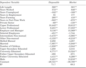
So far we have considered the relative welfare of men and women and the effect of educational qualifications. We are also interested in quantifying the effect of other characteristics on lifetime income and their components. In order to do this, we employ a regression method, taking the relevant equivalised market income or disposable income as regressor and various demographic, human capital and labour market characteristics as explanatory variables. We do not annualise income in this instance, so that we can determine the influence of life length on lifetime income.
influences on lifetime income. We also see that occupation has an important influence with, as expected, employers and managers or professionals, having the highest income, with non-manual workers having the lowest. The relationship with education is as expected, with higher education levels as shown in Table 4 being positively correlated with both market and disposable income. We also notice that being married has a negative influence on equivalised income. Although those in work are more likely to marry, as are those in the relatively higher earning occupations, these characteristics are likely to be correlated with other factors. Having children, because an equivalence scale is used, results in a lower standard of living than if the families did not have children.
Table 4: Ratio of Lifetime Income for each Education Level Achieved to the Average by Male and Female1
Male Female
LoSec UpSec Univ2 Total LoSec UpSec Univ2 Total
Disposable Income 57.3 80.4 133.2 100.0 53.5 74.2 128.8 100.0 Market Income 45.0 73.0 145.1 100.0 28.9 62.3 142.5 100.0 Income Tax 35.9 65.6 156.8 100.0 19.1 54.2 151.0 100.0 Social Insurance
Contributions 51.1 82.2 131.5 100.0 27.0 61.9 143.1 100.0 Income Levy 43.4 70.1 149.4 100.0 20.4 52.3 152.6 100.0 Pension Contributions 37.1 56.3 169.6 100.0 15.0 50.1 155.2 100.0 Social Assistance 195.9 140.4 30.5 100.0 258.5 128.2 56.5 100.0 Social Insurance 67.8 87.7 121.6 100.0 64.9 91.6 111.6 100.0 Child Benefit 157.4 97.9 95.1 100.0 218.3 104.0 83.2 100.0
Source: Author’s Calculations.
Note 1: Assumption (3) of Table 3 adopted.
2: LoSec – Lower Secondary, UpSec – Upper Secondary, Univ – Third Level.
Comparing the coefficients between market and disposable income, we can measure how the influence of different characteristics changes when the redistributive effect of the tax-benefit is included. Disposable income in this model is 20 per cent less on average than market income.12As a result, if these
characteristics had the same absolute effect on both types of income, then
coefficients would remain the same, with the constant coefficient adjusting by 20 per cent. This does not happen. The coefficient on the constant adjusts by the amount expected, but the relative contribution of the other characteristics changes. The impact of characteristics such as the labour market, human capital and gender fall in absolute terms as does the impact of children. All of these characteristics are important influences on income. The progressive nature of the tax-benefit system, will result in individuals with characteristics that positively influence income having their income reduced to a greater extent. Characteristics that are more likely to have lower incomes, will be more likely to receive benefits. The coefficients on life length and marriage increase. The longer an individual lives, the longer they will spend in retirement and hence the longer they will receive state benefits. Thus disposable income will increase relative to market income the longer they live.
Table 5: Characteristics that Influence Equivalent Lifetime Income
Dependent Variable Disposable Market
Life Length 590** 581**
Years Worked 572** 846**
Years Unemployed –102** –189**
Years in Employment 55 177
Years Farming 295** 410**
Years in Part-Time Work –503** –875**
Private Sector –69** –130**
Upper Professional 10,442** 19,612**
Lower Professional 9,231** 17,033**
Employer and Manager 9,116** 15,569**
Salaried Employees –451** –1,744
Intermediate Non-manual –3,475** –5,905**
Other Non-manual –3,155** –6,218**
Skilled Manual 2,258 4,257
Married –7,897** –5,948**
Number of Children –1,938** –2,844**
Upper Secondary Educated 1,258 2,315
University Educated 6,771** 13,524**
Father Upper Secondary Educated –492 –671 Father University Educated 4,411** 8,290**
Male 8,421** 13,616**
Constant –29,721** –39,790**
R2 71.7 68.2
Source: Author’s Calculations.
The Distribution of Lifetime Income
[image:18.595.116.475.260.443.2]In this section we examine the distribution of lifetime income and its composition. Table 6 describes the distribution of disposable income sub-com-ponents by quintiles of market income. Incomes are reported as a percentage of annualised equivalent market income. Annualised income is assumed to be shared equally between spouses in a family, and with the equivalence scale described in the previous section.
Table 6: Components of Annualised Lifetime Disposable Income over the Income Distribution (As a Percentage of Market Income)1
Market Income Quintile 1 2 3 4 5 Total
Market Income2 5.0 47.8 88.9 132.3 225.5 100.0
Tax-Benefit System 344.6 5.5 –14.1 –23.8 –32.6 –19.3 Income Tax –18.0 –21.2 –23.4 –26.2 –32.2 –27.7 Social Ins. Contrib. –1.8 –2.4 –2.7 –2.6 –2.0 –2.3 Income Levy –0.9 –1.4 –1.8 –1.9 –2.0 –1.9 Pension Contributions –0.7 –1.5 –1.5 –2.6 –2.9 –2.4 Social Assistance Benefits 244.9 12.6 4.2 2.3 1.5 5.7 Social Insurance Benefits 111.0 18.4 10.7 7.1 5.0 9.0
Child Benefits 9.9 1.2 0.5 0.3 0.1 0.4
Disposable Income Quintile 1 2 3 4 5 Total
Percentage of Males3 31.2 45.7 55.5 55.3 65.0 50.6
Average Life length3 75.1 73.6 75.9 76.8 79.6 76.2
Source: Author’s Calculations.
Notes: 1. Assumption 3 of Table (3) is used. 2. As a percentage of average market income. 3. Disposable income quintile used.
Income tax is the most important instrument in the tax benefit system. We notice the progressivity of the income tax system, where income tax as a percentage of market income rises by market income quintile.
The next most important instrument in terms of total size is social insurance benefits. Because eligibility for social insurance benefits depends upon having a work history, those in higher quintiles, receive on average more social insurance benefits. However, taken as a percentage of market income we find that social insurance is quite targeted, where the relative amount falls with lifetime income. This high degree of targeting is due to the absence of an earnings related component to the social insurance benefit system.
contributions. Social insurance contributions themselves are largely propor-tional across the income distribution. Because the social insurance system is not self-financing additional transfers are made from general progressive income taxation. Thus the social insurance system as a whole is quite redistributive.
As one would expect, means tested social assistance benefits are also targeted at the bottom of the income distribution. Although less important, child benefits too are proportionally more important to people at the bottom of the income distribution than at the top.
We also consider some of the characteristics of different individuals across the income distribution. For this, we utilise annualised equivalent disposable income quintiles as our ranking variable. We see that women are more likely, even under the assumption of shared income within a household, to be in the bottom of the income distribution. While two-thirds of the bottom disposable income quintile are female, two-thirds of the top quintile are males. Also we see that even though the quintiles adjust for life length, we see that average life length increases from quintile 2 to quintile 5. The average life length of quintile 2 is less than quintile 1 because of the greater reliance on benefits during retirement.
Lifetime Versus Annual Redistribution
We now compare the redistributive effect of the tax-benefit system taking the lifetime as the accounting period with an annual accounting period. In order to produce an annual income distribution, we utilise a similar method to Harding (1993) and Falkingham and Hills (1995). In a steady state, the distribution of the annual incomes over the lifetime of a single cohort will be comparable to the distribution of incomes of a cross-section. Therefore, we use the distribution of annual incomes over the lifetime of our cohort as our measure of the distribution of annual income.
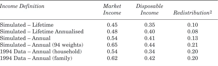
In Table 7 we consider the variability of disposable and market incomes as measured by the Gini coefficient and the degree of redistribution as measured by the Reynolds-Smolensky index (with reranking). As expected, because of the inequality reducing effect of public policy, disposable income for all income concepts is less variable than market income. We also see that lifetime incomes are less variable than annual incomes (market – 0.45 vs. 0.54; disposable – 0.35 vs. 0.41). This is due to the impact of income mobility over the life-course.
benefits at another point in the life-cycle. Income variability is higher and redistribution of the tax-benefit system is lower when lifetime incomes are annualised than when lifetime is considered unannualised.
Table 7: Inequality for Various Income Measures (Gini Coefficient)1
Income Definition Market Disposable
Income Income Redistribution2
Simulated – Lifetime 0.45 0.35 0.10
Simulated – Lifetime Annualised 0.48 0.40 0.08
Simulated – Annual 0.54 0.41 0.13
Simulated – Annual (94 weights) 0.65 0.44 0.21 1994 Data – Annual (household) 0.54 0.34 0.20 1994 Data – Annual (family) 0.62 0.42 0.20
Source: Author’s Calculations. Notes: For Non-annualised income, Assumption (2) of Table 3 is used. Otherwise Assumption (3) is used. Note1. For comparability reasons we simulate the 1998 tax-benefit system on the 1994 data. 2. Redistribution is measured by the difference between the Gini for Market income and the Gini for Disposable income, known as the Reynolds Smolensky Index (with reranking).
As an additional source of validation for the model, we compare the variability of simulated annual income with the variability of current income found in the data in 1994.13While the variability of market incomes is similar
(0.54 – 0.54), disposable incomes are much more variable for the simulated cohort than for the 1994 household population (0.41 – 0.34).
The difference between the simulated data and the survey data can be partially explained by the fact that in the simulated data, individuals are grouped into a narrower family unit, ignoring other household members. The survey-based measures meanwhile consider the wider household as the unit of analysis. As household sizes in Ireland are the largest in the European Union due to the presence of other non-dependentindividuals,14it is likely to have a
strong effect on the Gini-based measures used here.
Comparing the variability of incomes in the data when individuals are grouped into families, we see that the variability of both market and disposable incomes are higher, with data based disposable income variability being similar to the simulated variability (0.41 – 0.42). However, the vari-ability of market income is now quite different (0.54 – 0.62). However, as highlighted above, the simulated cohort has a very different population to the
13 Note that we update the 1994 market incomes to 1998 and then simulate the 1998 tax-benefit system.
1994 cross-section. Higher levels of education and improved economic circumstances result in more of the population in work in the simulated cohort than in the population cross-section. To try to make the simulated cohort more compatible with the 1994 data, we reweight the simulated cohort so that the education distribution is the same as that of the 1994 population. When we do this, we see that the variability of market (0.65 – 0.62) and disposable incomes (0.44 – 0.42) are broadly comparable in the simulated and survey data.15
[image:21.595.109.468.354.487.2]In Table 8 we consider the distribution of the components of disposable income by annual market income quintile. We must note that because there is no market income in the bottom quintile, we do not report this quintile. Comparing with Table 6 we can compare the degree of targeting of income components. The tax-benefit system taken as a whole is more targeted over the year than the lifetime. Income tax is marginally more progressive over a year than over the lifetime.
Table 8: Components of Annual Disposable Income over the Income Distri-bution (As a Percentage of Market Income)1
Market Income Quintile2 1 2 3 4 5 Total
Market Income3 0.0 15.6 85.4 139.5 259.5 100.0
Tax-Benefit System ∞ 142.5 –16.5 –25.1 –34.1 –19.9
Income Tax ∞ –17.9 –22.3 –25.0 –32.1 –28.0
Social Insurance Contributions ∞ –1.6 –2.4 –2.6 –2.1 –2.3
Income Levy ∞ –0.7 –1.6 –2.0 –2.0 –1.9
Pension Contributions ∞ –1.0 –1.5 –2.2 –2.9 –2.4
Social Assistance ∞ 48.3 2.8 1.4 1.4 5.6
Social Insurance ∞ 112.3 7.9 5.1 3.6 8.7
Child Benefit ∞ 3.1 0.7 0.2 0.0 0.4
Source: Author’s Calculations.
Notes: 1. Assumption 3 of Table (3) is used.
2. No Market Income in the bottom quintile and so disposable income component as a percentage of market income is infinite.
3. As a percentage of average market income.
Turning to benefits, we find that social assistance benefits are more targeted over a year than over the lifetime. Social insurance benefits are much less concentrated over the lifetime distribution than over the annual distribution. This is the best example of the influence of life-course mobility on the incidence of benefits. Because individuals are required to have a work
record to receive insurance benefits, long-term income for this group will be higher than for individuals who receive assistance benefits. Meanwhile if one focuses on a snapshotpicture of the population as a cross-sectional analysis does, because benefits are flat rate benefits and less than average income, these individuals will appear to be in the lower portion of the income distribution. The converse of this explanation gives the reason for the lack of difference between cohort and cross-section for assistance benefits.
Decomposition by Personal Characteristics
In the remainder of this section we consider the impact of personal characteristics on the distribution of lifetime income and the redistribution of taxes and benefits over the lifetime. Characteristics considered include Gender, Lifetime Labour Market Experience, Family Composition and Life-time duration. We use the method due to Morduch and Sicular (1998), described above to do this. In this part of the discussion we examine non-annualised incomes as we would like to investigate the influence of life length on redistribution.
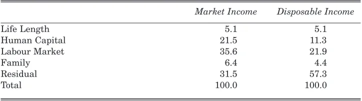
[image:22.595.114.476.500.601.2]The regressions reported above in Table 5 have been used as the basis of this method. Table 9 describes the contribution different categories make to overall inequality. We notice that for market income, labour market characteristics such as the number of years worked, the number of years unemployed and occupation etc. are the most important factors driving the variability in market income. Human capital is the next most important characteristic. Family characteristics such as the number of children account only for about 6 per cent of total variability.
Table 9: Decomposition of Income Variability into Personal Characteristics (as a Percentage of Total Variability)
Market Income Disposable Income
Life Length 5.1 5.1
Human Capital 21.5 11.3
Labour Market 35.6 21.9
Family 6.4 4.4
Residual 31.5 57.3
Total 100.0 100.0
Source: Author’s Calculations.
illustrates the impact the tax-benefit system has on reducing market inequalities. The contribution life length makes to this distribution is relatively limited at 5 per cent. This percentage remains the same for both measures. The impact of family on the variability of incomes also falls slightly.
V CONCLUSIONS
This paper assesses the redistributive effect of the Irish tax-benefit system over the lifetime. In order to generate a synthetic cohort to be used in this analysis, a dynamic microsimulation model is used. The principal conclusions are that broadly speaking the tax-benefit system over the lifetime redistributes from men to women, largely because of the income disparity between men and women in Ireland. This result is robust to assumptions about sharing between spouses within the household.
Overall the system redistributes from rich to poor, but the overall degree of redistribution over the lifetime is less than when income is based on shorter accounting periods such as a year. One of the principal reasons for this is because social insurance benefits are much less redistributive over the lifetime than at particular points in time. Because they are an insurance benefit, their object is to act as an income replacement mechanism during periods of low income. However, because they are dependent on previous income based contributions, individuals who become eligible for these benefits must have had sufficient previous contributions and by extension income to be eligible. As a result, especially for long-term instruments such as state pensions, these individuals will tend to be wealthier over the lifetime than individuals who do not meet these eligibility criteria, even though at one point in time when actually in receipt of these benefits they will be classified as poor.
In the final section we decomposed the inequality of incomes into the effect of personal income characteristics. The most significant result was the impact of the tax-benefit system in reducing the inequality due to the effect labour market history and human capital have on incomes.
this paper should be regarded as indicative of the type of analysis possible with a dynamic microsimulation model than as definitive analyses in their own right. It is likely to be the case that as the model is developed the values obtained may alter.
Because of these near-term shortcomings much of the effort has been spent in designing a flexible software framework in which the model is constructed. Although applications currently are quite limited, a primary objective has been to utilise a flexible design so that further applications can be exploited in the future such as simulating multiple cohorts to get a representative picture of the whole population rather than a single cohort. As an indication of the flexibility of the design, this dynamic modelling framework has been used to simulate expenditures in each of the European Union countries within the EUROMOD model (See Baldini et al., 2001). Other potential future applications include:
• Examining projected future income distributions under different economic and demographic scenarios.
• Evaluating the future performance of various governmental long-term programmes such as pensions, health and long-term care and educational financing.
• Designing new public policy by simulating the effect of potential reforms such as changes to education finance and pensions.
• Studying inter-temporal processes and behavioural issues such as wealth accumulation and the impact of tax-benefit systems on labour market mobility.
REFERENCES
ATKINSON, A. B. and J. MICKLEWRIGHT, 1991. “ Unemployment Compensation and Labour Market Transitions; A Critical Review”, Journal of Economic Literature, Vol. 29 No. 4
ATTANASIO, O. and J. BANKS, 1998. “Household Saving: Analysing the Saving Behaviour of Different Generations”, Economic Policy, Vol. 27 (October), pp. 549-583.
BALDINI, M., 1997. Diseguaglianza e Redistribuzione nel Ciclo di Vita, Bologna: Il Mulino.
BALDINI, M., D. MANTOVANI, and C. O’DONOGHUE, 2001. “Consumption Beha-viour and Indirect Taxation in Europe”, EUROMOD Working Paper no. 7/01, Department of Applied Economics, University of Cambridge.
BJÖRKLUND, A. AND M. PALME 1997. “Income redistribution within the life cycle versus between individuals: Empirical evidence using Swedish panel data”, Working Paper No. 197, Stockholm: Stockholm School of Economics.
BLOMQUIST, S., 1981. “A Comparison of Distributions of Annual and Lifetime Income: Sweden Around 1970,” The Review of Income and Wealth, Vol. 22, pp. 243-264. BURTLESS, G., 1996. “A Framework for Analyzing Future Retirement Income
Security” in E.A. Hanushek and N.L. Maritato (eds.), Assessing Knowledge of Retirement Behaviour, Washington D.C.: National Academy Press.
CALDWELL, STEVEN B., MELISSA M. FAVREAULT, ALLA GANTMAN, JAGADEESH GOKHALE, THOMAS JOHNSON, and LAURENCE J. KOTLIKOFF,1999. “Social Security’s Treatment of Postwar Americans” in James M. Poterba (ed.), Tax Policy and the Economy, Vol. 13. Cambridge, MA: National Bureau of Economic Research, MIT Press.
CALLAN, T., and B. NOLAN, 1990. “Income Distribution and Redistribution: Ireland in Comparative Perspective”, Working Paper Series No. 17. Dublin: The Economic and Social Research Institute.
CALLAN, T., B. NOLAN, B.J. WHELAN, C. T. WHELAN, and J. WILLIAMS, 1996. Poverty in the 1990s, Evidence from the 1994 Living in Ireland Survey, Dublin: Oak Tree Press in association with The Economic and Social Research Institute. CALLAN, T., and B. NOLAN 1999. “Income Inequality in Ireland in the 1980s and
1990s,” in F. Barry (ed.), Understanding Ireland’s Economic Growth, London: Macmillan Press.
CITRO, C. F. and E. A. HANUSHEK,1997. Assessing Policies for Retirement Income: Needs for Data, Research, and Models, Panel on Retirement Income Modelling, National Research Council.
EVANS, M. and J. FALKINGHAM, 1997. “Minimum Pensions and Safety Nets in Old Age: A Comparative Analysis”, Welfare State Programme Discussion Paper WSP/131. London School of Economics.
FALKINGHAM, J. and J. HILLS, 1995. The Dynamic of Welfare: The Welfare State and the Life Cycle. New York: Prentice-Hall.
HARDING, A. 1993. Lifetime Income Distribution and Redistribution: Applications of a Microsimulation Model, Amsterdam: North Holland.
IMMERVOLL, H. and C. O’DONOGHUE, 2001. “Towards a Multi-Purpose Framework for Tax-Benefit Microsimulation: A Discussion by Reference to EUROMOD, a European Tax-Benefit Model”, EUROMOD Working Paper no. 2/01, Department of Applied Economics, University of Cambridge.
HUGHES, G., 1985. Payroll Tax, Incidence, the Direct Tax Burden and the Rate of Return on State Pension Contributions in Ireland. General Research Series No. 120, Dublin: The Economic and Social Research Institute.
JARVIS, S. and S. JENKINS, 1998. “How much income mobility is there in Britain?”, Economic Journal,Vol. 108, pp. 428-443.
LAYARD, R., 1977. “On Measuring the redistribution of lifetime income”, in M. Feldstein and R.P. Inman (eds.), The Economics of Public Services. London: Macmillan.
NELISSEN, J. H. M., 1998. “Annual versus lifetime income redistribution by social security”, Journal of Public Economics, Vol. 68, No. 2, pp. 223-249.
O’DONOGHUE, C., 2001. Redistribution in the Irish Tax-Benefit System, unpublished PhD. thesis, London School of Economics.