On the vehicle sideslip angle estimation: a literature review of methods, models and innovations

of methods, models and innovations

CHINDAMO, Daniel, LENZO, Basilio <http://orcid.org/0000-0002-8520-7953>

and GADOLA, Marco

Available from Sheffield Hallam University Research Archive (SHURA) at:

http://shura.shu.ac.uk/18721/

This document is the author deposited version. You are advised to consult the

publisher's version if you wish to cite from it.

Published version

CHINDAMO, Daniel, LENZO, Basilio and GADOLA, Marco (2018). On the vehicle

sideslip angle estimation: a literature review of methods, models and innovations.

Applied Sciences, 8 (3), p. 355.

Copyright and re-use policy

See

http://shura.shu.ac.uk/information.html

sciences

Review

On the Vehicle Sideslip Angle Estimation:

A Literature Review of Methods, Models,

and Innovations

Daniel Chindamo1,*ID_{, Basilio Lenzo}2ID _{and Marco Gadola}1ID

1 _{Department of Industrial and Mechanical Engineering, Automotive Group, University of Brescia,}

I-25123 Brescia, Italy; [email protected]

2 _{Department of Engineering and Mathematics, Sheffield Hallam University, Sheffield S1 1WB, UK;}

[email protected]

* Correspondence: [email protected]; Tel.: +39-030-371-5663

Received: 8 January 2018; Accepted: 14 February 2018; Published: 1 March 2018

Abstract: Typical active safety systems that control the dynamics of passenger cars rely on the real-time monitoring of the vehicle sideslip angle (VSA), together with other signals such as the wheel angular velocities, steering angle, lateral acceleration, and the rate of rotation about the vertical axis, which is known as the yaw rate. The VSA (also known as the attitude or “drifting” angle) is defined as the angle between the vehicle’s longitudinal axis and the direction of travel, taking the centre of gravity as a reference. It is basically a measure of the misalignment between vehicle orientation and trajectory; therefore, it is a vital piece of information enabling directional stability assessment, such as in transience following emergency manoeuvres, for instance. As explained in the introduction, the VSA is not measured directly for impracticality, and it is estimated on the basis of available measurements such as wheel velocities, linear and angular accelerations, etc. This work is intended to provide a comprehensive literature review on the VSA estimation problem. Two main estimation methods have been categorised, i.e., observer-based and neural network-based, focussing on the most effective and innovative approaches. As the first method normally relies on a vehicle model, a review of the vehicle models has been included. The advantages and limitations of each technique have been highlighted and discussed.

Keywords:vehicle state estimation; vehicle dynamics; Extended Kalman Filter; Unscented Kalman Filter; GPS-aided estimation; neural networks

1. Introduction

Vehicle sideslip angle (VSA) estimation has been a big challenge since the introduction of the very first on-board active systems controlling vehicle stability, such as the electronic stability control (ESC, also known as ESP) in the early 1990s [1].

Nowadays, vehicle control systems (VCS) such as rear wheel steering, active steering, direct yaw moment control (DYC) through active differentials or torque vectoring, advanced traction controls, and the above-mentioned ESC (in all its forms) are used in conjunction to extend the vehicle performance and stability envelopes. They enhance road-holding capabilities, cornering performance, drivability, and ultimately stability, especially assisting the driver during emergency manoeuvres and in poor “grip” conditions [2–5]. All of these controls rely on vehicle state real-time assessments, and on VSA monitoring in particular. A fast and accurate estimation of the VSA can be considered a key to active safety, reducing the likelihood of dangerous events such as instability, loss of control, and roll-over, hence decreasing the number of accidents directly and abating the social impact of mobility.

The VSA is strongly related with the dynamic behaviour of ground vehicles. In purely kinematic terms, the VSA amplitude depends upon lateral acceleration, vehicle mass and mass distribution,

and rear axle slip angle; hence, it relies on properties such as rear tyre cornering stiffness, etc. [6]. Furthermore, it is well known that pneumatic tyres feature a typical, non-linear shape of side force versus slip angle characteristics due to saturation and load sensitivity. Consequently, a prompt action of VCS is imperative whenever their intervention is required. To put it simply, VCS should prevent the VSA from becoming large enough to digress into the tyre saturation range, otherwise, it might well be too late to “catch” the vehicle and restore driver control. This is even more important in low grip conditions, as tyre saturation might occur earlier, i.e., at very low slip angle values.

The VSA amplitude and its rate of change also provide primary driver feedback in conjunction with the so-called steering feeling [7,8], affecting perception and confidence in the vehicle, especially during turn-in and transients in general [4,9–11]. Efficient VSA monitoring is also vital for novel ADAS (Advanced Driver Assistance System) devices, as well as for the success of oncoming semi-autonomous and fully autonomous driving technologies [12]. The VSA in itself is often used for objective chassis design evaluation as well [13].

Vehicle dynamics researchers generally agree that the VSA can’t be measured directly for a series production vehicle. Unlike lateral acceleration or yaw rate, which are usually measured directly by means of low-cost sensors, the only way to accomplish a VSA measurement is to use an optical sensor such as the Corrsys–Datron [14]. Unfortunately, this sophisticated device is considered a research and development (R&D) tool rather than a sensor suitable for production vehicles, as it presents issues in terms of compatibility with vehicle packaging, cost, reliability, accuracy, and robustness to environmental conditions. With regard to motorsport, direct VSA measurement on racing cars is often forbidden by the sporting regulations issued by the governing body. Therefore, VSA cannot be measured on everyday cars, and a reliable estimation process is required to feed important active safety systems such as the ESC.

For all these reasons, VSA estimation continues to attract considerable interest in the academic and industrial worlds. As a matter of fact, it is well known that research on active safety technologies in general can have a considerable impact on social life by preventing or reducing the potential severity of casualties. The relevance of this topic in particular has been proven by the very large number of papers that have appeared in the literature over the past 30 years, often involving other subjects such as vehicle dynamics, tyre modelling, theory of control, data fusion, instrumentation, human behaviour, and human–machine interaction. To give an example, Crolla already proposed a review on the theme back in 2007 [2]. Also, renowned authors such as Cheli [15,16], Best [13], and Rajamani [17] provide significant contributions that present varied techniques and achievements. From all of the above, the authors felt the need to propose an updated review of the most significant contributions in recent years.

To date, among the many VSA estimation strategies proposed, none have succeeded to be considered the most effective or the most accurate. To provide clarity in the subject, we present an extensive review of the techniques, strategies, models, and methods that have been published in the literature. A total of 119 studies on this topic have been reviewed.

Two categories of VSA estimation have been identified:

later on in this paper, this method already provides satisfactory results, and better results are likely to be achievable due to the expected increase in the accuracy and reduction in cost of the GPS receivers. On the other hand, GPS receivers present issues such as temporary signal unavailability due to surroundings such as trees, tall buildings, and road tunnels, as well as different working frequencies with respect to other sensors involved in vehicle dynamics control (i.e., accelerometers, gyros, etc.) [68].

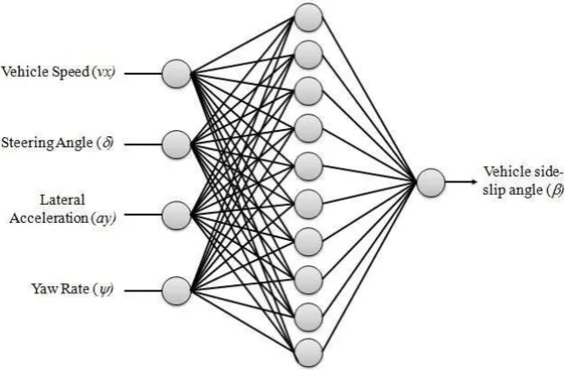
• _{Neural network-based [96–110]: This method is specifically used to overcome the need for a} vehicle model of any kind and its related complex set of parameters [101]. Artificial neural networks (ANN) are largely considered effective tools for system modelling, as they are suitable to model complex systems using their ability to identify relationships from input–output data pairs. They also offer decisive advantages such as adaptive learning, fault tolerance, and generalisation. Moreover, in recent years, the development of high speed computers encouraged the application of ANN, which has progressed very quickly. Using an ANN, the vehicle can be considered as a black box system, and only a conventional set of sensors is needed to train/feed the network. In this case, the inputs for the black box are the yaw rate, lateral acceleration, steering angle, and vehicle speed, while the VSA is the output. Estimation results are accurate as much as the training dataset contains the whole possible scenario that the system might have to deal with [96]. This method has a major drawback, consisting in the need of changing the ANN every time the system changes, forcing the user to redo the ANN training procedure. This is probably the reason why the use of ANN seems to be a second choice for VSA estimation. This is reflected in the literature production, where not so many works can be found on this approach.

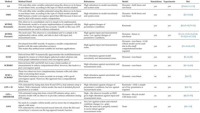
The paper is organised as follows: Section2analyses observer-based estimation, presenting the different types of observers with a specific focus on the most used ones, vehicle model applications, and GPS-aided observers. Section3 concerns the neural network-based estimation. A detailed overview table on the existing VSA estimation methods is presented in Section4, where concluding remarks are also given. Hardware costs, computational burden, and accuracy are also taken into account in order to assess the efficiency of each approach.

2. Observer-Based Estimation

As far as the VSA estimation is concerned, three state observers are found in the literature: the Luenberger observer (LO), the sliding-mode observer (SMO), the Kalman filter (KF), and their variants. All of them can be used both for linear and non-linear systems. As discussed, observers are based on a vehicle model; therefore, Section2.1analyses the most used vehicle models. Owing to the KF being the most used observer (71 studies out of 120 observer-based in total), a general description of the LO and SMO is provided hereafter, whilst a full section, i.e., Section2.2, is dedicated to the KF method. Finally, Section2.3discusses the potential use of GPS to enhance observer-based estimation.

In summary, the most used observer for VSA estimation is the KF, due to its ability to use input and measurement noise information directly, and because it is robust, stable, and relatively simple to implement [15,18,19].

2.1. Vehicle Models

Two kinds of model can be found in the literature, which are denoted respectively as kinematic and dynamic. On the one hand, the kinematic model is concerned with the vehicle motion with no reference to forces; thus, it does not need complex parameters such as those regarding tyres. Figure1

depicts a vehicle model showing: the vehicle velocity at the centre of gravity (G)VG, the longitudinal

and lateral components ofVG, respectivelyuandv, the vehicle yaw rater, the VSAβ, the vehicle

trackt(here assumed to be the same for the front and the rear), the front and rear semi-wheelbases, respectivelya1anda2, and the vehicle wheelbasel.

β

= +

= + =d_{d =} + _{d +}d + _dd

d d = d d = −

Figure 1.Kinematic modelling of a vehicle [113].

The vehicle velocity can be written as:

VG=ui+vj (1)

whereiandjare unit vectors that are aligned respectively with the vehicle longitudinal axisxand the vehicle lateral axisy(local reference frame). The acceleration of the vehicle at the centre of gravity is, by definition:

aG=axi+ayj= dVG

dt = .

ui+udi dt+

. vj+vdj

dt (2)

whereaxandayare, respectively, the longitudinal and lateral acceleration of the vehicle. Since the

local reference frame rotates with the vehicle body, from Poisson’s formulae [114]:

di

dt =rj

dj

dt =−ri

(3)

ax=

. u−_vr ay=

.

v+ur (4)

An observer based on a kinematic vehicle model uses Equation (4) to estimate u and v (see Section2.2); therefore, the sideslip angle would be, by definition (see Figure1):

β=tan−1v u

(5)

Some authors introduce the hypothesis of a small sideslip angle,β≪_{1. If so, sinβ}≈_{β, cosβ}≈_1, andv ≈ _{uβ; hence, the overall vehicle speed would beV =} u

cosβ ≈u. Using .

v ≈_(u._{β) = u}._β+β._u, one can easily rearrange Equation (1) to obtain the following expression, providing the VSA by integration [16]:

.

β≈ ay

u −

ax

u −r (6)

The main issue of VSA estimation using a kinematic model is that it does not work when the vehicle yaw rate is relatively small or zero, as the system becomes unobservable [116,117].

The dynamic model, on the other hand, provides a more detailed description of the vehicle dynamics, as it is based on the equilibrium equations. Considering the vehicle as a rigid body, the following is a generic set of equilibrium equations [118,119]:

max=m

. u−_vr

=

px

∑

i=1 Fx,i

may=m

. v+ur

=

py

∑

i=1 Fy,i

Jz

. r=

pz

∑

i=1 Mi

(7)

where m is the vehicle mass, Jz is the vehicle moment of inertia with respect to a vertical axis,

Fx,iandFy,iare the generic force contributions, respectively, in the vehicle longitudinal and lateral

direction, andMi is the generic yaw moment contributions. A dynamic model can have different

levels of detail/complexity and hypotheses used, with all of them affecting the estimation accuracy. As an example, adopting a standard four-wheel model, as shown in Figure2, the three equilibrium equations are:

max=m

. u−_vr

=Fx11cosδ11+Fx12cosδ12−Fy11sinδ11−Fy12sinδ12+Fx21+Fx22 may=m

. v+ur

=Fy11cosδ11+Fy12cosδ12+Fx11sinδ11+Fx12sinδ12+Fy21+Fy22 Jz

.

r= Fx12cosδ12−Fy12sinδ12+Fx22−Fx11cosδ11+Fy11sinδ11−Fx21₂t + Fy11cosδ11+Fy12cosδ12+Fx11sinδ11+Fx12sinδ12a1− Fy21+Fy22a2

(8)

whereδ11andδ12are the wheel steering angles, respectively the front left and front right,FxijandFyij









∈ ℜ

=

,

,

= ℎ

,

Figure 2.Dynamic modelling of a vehicle, with road-tyre force [113].

Although some papers use relatively complete vehicle models, several studies introduce simplifying hypotheses, such as:

• _{the use of single track vehicle models (also known as the bicycle model), e.g., [16,24,120] by} Cheli et al., Gadola et al. and Naets et al.;

• _{the assumption of the availability of the vehicle longitudinal speed, so that the first equation in} Equation (7) is not used, e.g., [16,24,26] by Cheli et al., Gadola et al., Chen et al.;

• _{the assumption of small steering angles and/or small sideslip angles, e.g., [16,26] by Chen et al.} and Cheli et al.;

• _{no road inclination and/or bank angle (only a few papers address these issues, e.g., [32,58,121] by} Grip et al., You et al., and Ryu et al.

2.2. Kalman Filter

The KF, along with its variants (extended Kalman filter and unscented Kalman filter), addresses the general problem of trying to estimate the state vectorx ∈ ℜn_{of a discrete-time controlled process}

that is governed by the generic set of equations [126]:

xk= f(xk−1,uk−1,wk−1)

zk=h(xk,vk)

(9)

whereuis the system input,zis the system output (i.e., the measured variables), andvandware respectively the process and measurement noises. The process noise is introduced to account for the (unavoidable) difference between the dynamics of the actual system and the model used to represent it. Ideally, should a model be exactly representative of a system,wwould be zero. Similarly, measurement errors are accounted for inv, which depends on the accuracy of measurements (e.g., the quality of the sensors used). The noises are assumed to have a Gaussian distribution with zero mean and covariances

QandR, respectively, forwandv.

The idea of a KF is that the state vectorxkcould be estimated in two independent ways: (i) using

the first equation in Formula (9), i.e., the dynamic evolution of the system; or (ii) using the second equation in Formula (9), inverting it to work outxk. However, both estimations would be affected

by an error, depending on (i) the reliability of the model (parameters, unmodeled effects etc.); and (ii) the reliability of the measures. These reliabilities depend respectively onQandR. The KF simply computes a weighted average between the two estimations of the state vector, the weight depending on

QandR, which is calculated in order to minimise the covariance of the estimation error. The estimation error is the difference between the estimated state and its (unknown) actual value [126].

If the system is linear, then Formula (9) can be written in the form:

xk= Axk−1+Fuk−1+wk−1

zk=Hxk+vk

(10)

Denoting with ˆxk−the state estimate at stepkaccording to the dynamic evolution of the system

(the first equation in Formula (10)), the KF estimation is:

ˆ

xk=xˆk−+K(zk−Hxˆk−) (11)

One form ofKis given in [126] by Welch et al., and depends onQ andR. For example, ifR

approaches zero, i.e., in the hypothesis of an extremely reliable measurement, thenK≈ _H−1_{; hence,} ˆ

xk ≈ H−1zk. If the system is not linear, i.e., it can be described only in the general form (as in

Formula (9)), it can be linearised and written in a form similar to Formula (10). Such approach is known as an extended Kalman filter (EKF).

In [20], a comparison between EKF and SMO has been performed considering a non-linear heavy vehicle model, and the results showed that both methods were sufficiently accurate, but SMO has been preferred since it requires less input measurements. However, the KF is very simple to be used and implemented; moreover, its robustness, stability, and ability to deal with input and measurement noise make it the most used observer for VSA estimation [18]. This statement is also supported by [25], where after a comparison between the EKF, LO, and SMO concerning the VSA estimation using a non-linear single-track model, EKF achieved a smaller estimation error than the LO and SMO.

Nonetheless, as discussed in Section2.1, should the conditions change (e.g., due to tyre wear) with respect to the modelled ones, again, the performance of the estimation would be unsatisfactory. Some authors [13,18,31] tried to overcome the problem by using a simple single-track model with cornering stiffness adaption. Results show that VSA estimation is very close to the actual value except for some VSA peaks, where the estimated VSA values deviate from the actual values. That is, due to simplified tyre models that operate only in the linear zone (adapting the cornering stiffness to expand its usage range) but neglecting the non-linear and saturation zone behaviour. In a similar work [24], the tyre model adaption regards the entire non-linear range. By using a standard family of curves representing a generic Pacejka model dataset and an integrated tuning procedure for the EKF observer, the authors managed to develop a tyre model that was consistent with the lateral behaviour. The tuning is performed with respect to a single parameter that is easy to set. This allows the use of a simple vehicle model without detailed knowledge of the whole number of parameters related to the tyres fitted on the vehicle, while taking the non-linear saturation tyre behaviour into account. Results showed an error under 5% in every tested manoeuvre, as well as benefits in terms of computational burden, hence its suitability for real-time applications. Ahangarnejad et al. in [122] proposed a dual extended Kalman filter (DEKF) approach, where two EKFs are used in parallel. The first EKF is used to estimate the vehicles states, including VSA. The second EKF is used to estimate the parameters of a rational tyre model, which are then fed to the first EKF for the vehicle state estimation. Naets et al. in [120] introduces a non-linear least squares tyre parameter estimator that is able to run online (but not in real-time).

The EKF has two major drawbacks that consist of the high computational effort required in the definition of the Jacobian matrices, and its intrinsic linearization errors, which force the use of very small sampling times.

An effective solution to reduce the computational burden while keeping a high accuracy in the VSA estimation is the use of the unscented Kalman filter (UKF) instead of the EKF [33–39]. As a matter of fact, many recent observer-based studies on VSA estimation mostly focused on UKF [33,35,37,38].

The UKF observer is based on the approximation of random statistic variables using the definition of sigma points [127]. These points are then propagated through the (non-linear) system equation yielding some random variables of a non-linear stochastic description. Afterwards, such variables are approximated by a Gaussian random function, enabling the use of the standard equation for Kalman gain calculations.

A great benefit is that a UKF does not require the computation of Jacobian matrices, which makes it particularly suitable for systems with high non-linearities. The UKF achieves higher accuracy if compared to the EKF, while requiring similar effort in terms of computational load. On the other hand, the system complexity increases significantly. Several additional parameters are introduced, such as the number of sigma points, their positioning, and the weights used to compute the final estimation [127]. For instance, Antonov et al. in [36] explains that the set of sigma points must be cautiously chosen and weighed to approximate the vehicle state appropriately. Therefore, a very careful and thoughtful tuning is needed for a successful implementation of a UKF, while an EKF is generally simpler.

to a degradation of the observer estimation capabilities. On the other hand, a longer sample time means less computational effort required, and hence a better suitability to real-time applications or the possibility to use cheaper hardware without jeopardising the final estimation performance.

Some remarkable VSA estimation via UKF application can be found in [38] by Ren et al., where a simple four-wheel, three-DOF vehicle model was improved by using a linear, piece-wise tyre model that describes the Dugoff model using less parameters then the traditional Dugoff model. Results are promising; however, the authors validate this method via CarSim simulations only. In [36] by Antonov et al., the same vehicle model (except for the tyres, which are represented by means of the Magic Formula) was used with a separate calculation of tyre vertical forces to enhance the estimation without affecting the computational effort required. They also use a BMW sedan to perform some aggressive high-speed low-friction manoeuvres in order to verify the accuracy and robustness of the proposed method. The results showed good accuracy, even in extreme driving situations. In this case, a comparison between EKF and UKF has been reported, and results show that the EKF observer was outperformed by the UKF.

Moreover, in [35] Chen et al. shows a further improvement of UKF, where an UKF-based adaptive variable structural observer with dynamic correction has been presented. Basically, model uncertainty has been compensated with adaptive parameters, while a variable structure observer has been realised through using a sensor-based observer to compensate errors occurring in non-linear regions.

An improved KF has also been proposed in [40] by Li et al. It has been achieved by merging the estimation outputs of two KF variants, namely the square-root cubature Kalman filter (SCKF) and the square-root cubature-based receding horizon Kalman filter (SCRHKF). The first one numerically approximates the multidimensional integrals by means of a third-degree spherical-radial cubature rule; it features good accuracy and high convergence speed, but accuracy may be reduced by model uncertainty and noise [41,42,49]. On the other hand, SCRHKF is robust against uncertainty and noise, but due to the use of a finite number of measurements, its convergence speed is slower than SCKF. Therefore, SCKF and SCRHKF have features that are complementary with each other. Hence, Li and Zhang [40] proposed a hybrid KF for VSA estimation that integrates the advantages of the two filters mentioned above while overcoming their issues. They verified the accuracy of this method by performing double lane change manoeuvres with a real-world vehicle at several speeds. Estimation results have been accurate, since they show a low RMS error in steady state manoeuvres, and low maximum error at peaks as well. However, this approach still has potential issues in terms of computational effort.

the history of three signals: steering angle, lateral acceleration, and yaw rate, with a larger weight on the latter.

2.3. GPS-Aided Estimation

A previous extensive review of VSA estimation through GPS-aided methods has been recently carried out by Leung et al. [68]. For the sake of brevity, readers are invited to refer to Leung’s work. Nevertheless, some important considerations are worth highlighting.

The majority of the GPS-aided methods studied in the literature use a simple dynamic vehicle model with linear tyres (due to its simplicity) with an EKF as an estimator aided with GPS data [75–87]. Also, the most recent works, i.e., those published after Leung’s work, are focussed on this strategy [88–93], rather than the use of a kinematic vehicle model. They all obtained promising results, especially those who have further extended the GPS use to investigate tyre–road friction [89,93], roll, and banking angle [94], or with a dual GPS setup [74,91].

It is worth noticing that some major issues come into play with this approach. First of all, GPS receivers suffer from high price, low update frequencies, and sensitivity to the external environment. They are also sensitive to surroundings (e.g., trees or buildings), which can cause temporary outages. As a matter of fact, in most cases, vehicle dynamics sensors such as accelerometers and gyros operate at 100 Hz. However, due to hardware limitations, GPS receivers can operate at most at 50 Hz, whilst cheaper devices suitable for this application operate at less than 10 Hz only. Therefore, any dynamical changes in between samples are undetectable. Higher-sampled GPS are available, but their cost rises exponentially with the sample rate. The difference between the two sampling rates leads to an error during the inertial sensors (IS) and the GPS fusion process, since IS measurements are forced to be down-sampled in order to be synchronised with GPS.

Leung et al. [68,95] reported a simple way to overcome the problem. They suggested fitting a second-order curve on the down-sampled VSA estimation in real-time in order to provide a continuous estimation between GPS samples as well, without affecting the computational burden required. This method showed some overshooting problems during sudden changes in vehicle lateral velocity, but it is helpful to solve the issue regarding discontinuity in the VSA estimation.

A different solution to overcome the low sampling rate issue has been proposed by Bevly [70,71,81]. This method uses a KF, together with the data fusion from GPS and IS, to predict the IS biases when GPS data are available, and integrate the “corrected” IS signals when such data become unavailable. Hence, this allows the estimation of IS biases as well as the attenuation of the errors (drifts) in the sensor signal.

However, Bevly et al. in [70,71,81], proposed a single GPS receiver is used, resulting in the ability to predict the gyro bias only when the vehicle is travelling straight. A dual GPS antenna setup is therefore introduced by Bevly et al. in [82] and Ryu et al. in [83] that allows the yaw angle to be measured at any instant.

3. Neural Network-Based Estimation

The use of the so-called soft computing techniques such as artificial neural networks, genetic algorithms, and fuzzy logic is increasingly widespread in engineering applications e.g., [128] by Chindamo et al.

Figure 3.Artificial neural networks (ANN) estimation process high-level schematic.

Most of the authors who have addressed this topic used the same general approach. It consists of a three-layered neural network composed by one input layer, one hidden layer, and the output layer, where the first and second layer’s neurons use the log–sigmoid transfer function, while in the third layer, neurons use the linear functions. For the sake of clarity, inputs are considered those signals that can be easily measured on board any vehicles such as the yaw rate, lateral/longitudinal acceleration, vehicle speed, and steering angle, while the only output is the VSA. This kind of layered ANN with at least two layers is also able to memorise any kind of non-linear model [97,103]. Figure4shows the general layout of the above-mentioned ANN.

Figure 4. General layout of an ANN used for vehicle sideslip angle (VSA) estimation. Figure 4.General layout of an ANN used for vehicle sideslip angle (VSA) estimation.

A comprehensive training dataset is required to obtain a good estimation using an ANN. Except for [99] by Yu, which uses a radial basis function (RBF), they use the consolidated Levenberg–Marquardt back-propagation (BP) algorithm along with the mean squared error (MSE) performance index to train the ANN. This BP optimisation algorithm updates the weights and biases of the network, as presented in [129,130] by Levenberg and Marquardt, while the RBF is a feed-forward propagation method that requires less calculation, with a faster learning process [100].

special linear layer that computes the weighted output of the first layer. Particularly, Wei et al. in [106] tested this ANN on many handling manoeuvres, obtaining a fast response with high estimation accuracy. However, they did not investigate the robustness of this method against varying speeds and changing conditions (adherence, for instance).

However, some studies suggest another strategy to improve efficiency and reliability. In [101] Chindamo et al. for example, a single special training manoeuvre has been suggested to improve the ANN estimation capability, while keeping its structure simple to avoid computational burden issues, as 10 neurons were used in the hidden layer. Such a manoeuvre consists in a 45◦sine steer performed at increasing speed from 5 km/h to 100 km/h using a 15 km/h/min slope to be performed in at least three different friction conditions (i.e.,µ= 1, 0.5, 0.2). This method produced very good estimation results; however, it was only tested via a CarSim Simulation, as a real-world test would be quite complicated due to the extension of the proving ground required.

Furthermore, Melzi et al. [96] proposed the basic ANN that was described at the beginning of this section with the addition of a feedback line with the value of the VSA estimated by the network (only in the testing phase, with no feedback line during the training phase indeed). The VSA was introduced with an 8x∆_{ttime delay. In fact, they assert that the presence of the correct target among} input variables would have assigned to the output a value of 1-VSA and 0 to all of the other signals, driving the ANN to a VSA estimation without considering the complete vehicle dynamics becoming unreliable if applied to a manoeuvre that was not present in the training dataset. Thus, the introduction of the time delay was aimed at reducing the relative weight of the VSA in the ANN. To verify the reliability of their method, they performed many tests at various speeds using a real-world vehicle on different adherence friction conditions. They found that the ANN was able to predict the VSA accurately in transient conditions, while the results were not acceptable for steady-state or near-steady state conditions due to the estimation drift caused by the feedback line. The same ANN without the feedback line can only give good a VSA approximation in driving conditions that are far from the vehicle limit of adherence.

In another promising work, Broderick et al. [104] trained an ANN with a set of manoeuvres in order to take into account a shift in vehicle weight, a change in road surface, and a radical change in tyre characteristics. However, the training procedure is highly time demanding, and they only tested the network on two scenarios.

Also, Acosta et al., Dye et al., Alagappan et al. and Huang et al in [107–110] used a hybrid estimator composed by a neural network and an observer (typically an EKF). The first one has only the task of fitting tyre data, while the second estimates vehicle dynamics states. In these works, the ANN structure is the simplest possible in order to avoid an undesired increase of the computational burden.

The main issues of the ANN-based estimation remain the inability of the network to deal with a change in the vehicle after the training procedure, and the possibility of dealing with a road banking angle, which must be estimated with an external algorithm [129], and then, as proposed in [98,102], filtering out the lateral acceleration component due to gravity.

4. Conclusions

Table 1.Recap based on method and approach adopted for vehicle sideslip angle (VSA) estimation. LO: Luenberger observer; SMO: sliding-mode observer; KF: Kalman filter; EKF extended Kalman filter; UKF: unscented Kalman filter; SCKF: square-root cubature Kalman filter; SCRHKF: square-root cubature-based receding horizon Kalman filter; IS: inertial sensors.

Method Method Detail Robustness Model Simulations Experiments Ref.

LO VSA and other state variables estimated using this observer in its linear or non-linear form, according to the type of vehicle model adopted

High robustness to model uncertainty and system noise

Dynamic—both linear and

non-linear yes yes [59,60,111,112]

SMO

VSA and other state variables estimated using this observer in its linear or non-linear form, according to the type of vehicle model adopted. SMO features a faster convergence speed than EKF, because it does not need to deal with massive matrix computation.

High robustness to model uncertainty and system noise

Dynamic—both linear and

non-linear yes yes [20–23,60]

KF/EKF, Kinematic

This observer is consolidated, and it is simple to be implemented. The kinematic model is of easier implementation if compared with the dynamic model, but generally less accurate. Usually in this case, GPS measurements are used to enhance estimation.

High against changes of

parameters/conditions Kinematic yes yes [40,43–48,79–81]

KF/EKF, Dynamic

The most used. This observer is consolidated and it is simple to be implemented, robust, stable, and able to deal with input and measurement noise.

High against input and measurement noise. Low against changes of parameters/conditions.

Dynamic—linear or

non-linear yes yes

[13,16–19,24–32,47,48, 50–58,61–67,120]

UKF

Developed from EKF recently. It requires a smaller computational burden with the same estimation accuracy.

This makes this method more suitable for real-time applications.

High against input and measurement noise.

Dynamic—non-linear. A full vehicle model can be used due to the small computational burden required

yes yes [33–43,46,127]

SCKF

Derived from EKF. It numerically approximates the multidimensional integrals by means of a third-degree spherical-radial cubature rule. It has proper estimation accuracy and convergence speed.

Low robustness against model

uncertainty and measurement noise. Dynamic—non-linear yes yes [41,42,49]

SCRHKF

Derived from EKF and SCKF, but it uses a finite number of

measurements to reduce computational effort; however, this leads to a poor convergence speed.

High robustness against uncertainty and

measurement noise. Dynamic—non-linear yes yes [40–42,49]

SCKF + SCRHKF

These two observers have complementary features with each other while overcoming their issues.

This hybrid estimator is more accurate on average, with a good convergence speed. However, this approach has a computational effort issue.

High robustness against uncertainty and

measurement noise. Dynamic—non-linear no yes [40,67]

GPS + IS

VSA estimated by fusing data from IS and GPS (a dual antenna setup is better). With a kinematic vehicle model, the need of detailed physical parameters is avoided.

High robustness against changes of parameters/conditions, but low against measurement noise.

Kinematic—Only a simple set of few parameters is required

no yes [68–74]

GPS + OBSERVER

VSA estimated using data from a dual GPS antenna setup, and a dynamic model with an observer to provide continue estimation during GPS outages.

High—the observer (usually an EKF) gives high robustness against input and measurement noise.

Dynamic—Bicycle model

with linear tyres no yes [68,75–95]

ANN

No need of a complex vehicle model, and no errors due to integration of signals with noise.

VSA estimated by a three-layered neural network where the first and second layer’s neurons use the log-sigmoid transfer function.

Very low against system and external condition changes (i.e., grip). When the network is properly trained, it can be robust against

measurement noise.

The observer-based approach has been found to be the most used (71 works out of 120). It heavily depends on the kind of vehicle model, its accuracy, and the completeness of its set of parameters. The computational burden can also be an issue; nevertheless, the method can lead to very accurate results. GPS-aided methods are often combined to an observer, using the GPS data to overcome any estimation gaps or inaccuracy. However, GPS sampling frequencies, availability, and cost should also be considered during the design of a VSA estimation system.

The neural network-based approach has been specifically designed to overcome the need of a vehicle model and be suitable for a real-time environment, since it does not require much computational effort. In this case, the poor capability of the ANN to deal with any environmental or vehicle physical changes (for example, tyre wear or road friction) cannot be neglected.

In all cases, the cost-to-accuracy ratio plays an important role in choosing the correct estimation method.

Author Contributions:D.C. conceived this work as a review. D.C., B.L. and M.G. wrote the paper.

Conflicts of Interest:The authors declare no conflict of interest.

Nomenclature

VSA Vehicle sideslip angle ESP Electronic Stability Program VCS Vehicle Control Systems GPS Global Positioning System LO Luenberger Observer IS Inertial Sensors

SMO Sliding Mode Observer ANN Artificial Neural Network KF Kalman Filter AI Artificial Intelligence EKF Extended Kalman Filter MSE Mean Squared Error UKF Unscented Kalman Filter RBF Radial Basis Function SCKF Square-root Cubature Kalman Filter BP Back Propagation SCRHKF Square-root Cubature Based Receding Horizon KF GRNN General Regression NN ANFIS Adaptive Neuro-Fuzzy Inference System NN Neural Network

ax Longitudinal acceleration C Centre of gravity-rear axle distance

ay Lateral acceleration B Centre of gravity-front axle distance

u Longitudinal speed T Front/rear track

v Lateral speed L Wheelbase

α Tyre slip angle xk State vector

β Vehicle slip angle zk Output vector V Overall vehicle speed uk Input vector

r Yaw rate wk Measurement noise

m Vehicle mass vk Process noise

Fx Tyre longitudinal force A State transition matrix

Fy Tyre lateral force F Control-input model matrix

FAERO Aerodynamic drag force H Observation model matrix

Jz Vehicle yaw inertia Q Process error covariance matrix

M Yaw moment R Measurements error covar matrix

δ Wheel steering angle

References

1. Van Zanten, A.T.Bosch ESP Systems: 5 Years of Experience; Technical Paper 2000-01-1633; SAE International: Warrendale, PA, USA, 2000.

2. Manning, W.J.; Crolla, D.A. A review of yaw rate and sideslip controllers for passenger vehicles.Trans. Inst. Meas. Control2007,29, 117–135. [CrossRef]

3. Shibahata, Y.; Shimada, K.; Tomari, T. Improvement of vehicle maneuverability by direct yaw moment control.Veh. Syst. Dyn.1993,22, 465–481. [CrossRef]

4. Lenzo, B.; Sorniotti, A.; Gruber, P.; Sannen, K. On the experimental analysis of single input single output control of yaw rate and sideslip angle.Int. J. Automot. Technol.2017,18, 799–811. [CrossRef]

6. Mastinu, G.; Ploechl, M.Road and Off-Road Vehicle System Dynamics Handbook; Mastinu, G., Ploechl, M., Eds.; CRC Press: Boca Raton, FL, USA, 2014.

7. Gritti, G.; Peverada, F.; Orlandi, S.; Gadola, M.; Uberti, S.; Chindamo, D.; Romano, M.; Olivi, A. Mechanical steering gear internal friction: Effects on the drive feel and development of an analytic experimental model for its prediction. In Proceedings of the International Joint Conference on Mechanics, Design Engineering & Advanced Manufacturing, Catania, Italy, 14–16 September 2016; Springer: Cham, Switzerland, 2016; pp. 339–350.

8. Crema, C.; Depari, A.; Flammini, A.; Vezzoli, A.; Benini, C.; Chindamo, D.; Gadola, M.; Romano, M. Smartphone-based system for vital parameters and stress conditions monitoring for non-professional racecar drivers. In Proceedings of the 2015 IEEE SENSORS, Busan, Korea, 1–4 November 2015; IEEE: Piscataway Township, NJ, USA, 2015.

9. Gillespie, T.D. Fundamentals of Vehicle Dynamics; SAE International: Wattendale, PA, USA, 1992; ISBN 1-56091-199-9.

10. Marchesin, F.P.; Barbosa, R.S.; Alves, M.A.L.; Gadola, M.; Chindamo, D.; Benini, C. Upright mounted pushrod: The effects on racecar handling dynamics. InThe Dynamics of Vehicles on Roads and Tracks: Proceedings of the 24th Symposium of the International Association for Vehicle System Dynamics, Graz, Austria, 17–21 August 2015; CRC Press: Boca Raton, FL, USA, 2015; pp. 543–552.

11. Benini, C.; Gadola, M.; Chindamo, D.; Uberti, S.; Marchesin, F.P.; Barbosa, R.S. The influence of suspension components friction on race car vertical dynamics.Veh. Syst. Dyn.2017,55, 338–350. [CrossRef]

12. Hu, C.; Wang, R.; Yan, F.; Chen, N. Should the Desired Heading in Path Following of Autonomous Vehicles be the Tangent Direction of the Desired Path?IEEE Trans. Intell. Transp. Syst.2015,16, 3084–3094. [CrossRef] 13. Best, M.C.; Gordon, T.J.; Dixon, P.J. Extended Adaptive Kalman Filter for Real-time State Estimation of

Vehicle Handling Dynamics.Veh. Syst. Dyn.2000,34, 57–75.

14. Datron Technology Home Page. Available online: http://www.datrontechnology.co.uk/(accessed on 19 September 2017).

15. Cheli, F.; Melzi, S.; Sabbioni, E. An adaptive observer for sideslip angle estimation: Comparison with experimental results. In Proceedings of the ASME International Design Engineering Technical Conferences and Computers and Information in Engineering Conference, Las Vegas, NV, USA, 4–7 September 2007; ASME: New York, NY, USA, 2007.

16. Cheli, F.; Sabbioni, E.; Pesce, M.; Melzi, S. A methodology for vehicle sideslip angle identification Comparison with experimental data.Veh. Syst. Dyn.2007,45, 549–563. [CrossRef]

17. Piyabongkarn, D.; Rajamani, R.; Grogg, J.A.; Lew, J.Y. Development and experimental evaluation of a slip angle estimator for vehicle stability control.IEEE Trans. Control Syst. Technol.2009,17, 78–88. [CrossRef] 18. Dakhallah, J.; Glaser, S.; Mammar, S. Vehicle Sideslip Angle Estimation with Stiffness Adaption.Int. J. Veh.

Auton. Syst.2010,8, 56–79. [CrossRef]

19. Katriniok, A.; Abel, D. Adaptive EKF-Based Vehicle State Estimation with Online Assessment of Local Observability.IEEE Trans. Control Syst. Technol.2016,24, 1368–1381. [CrossRef]

20. Dakhallah, J.; Imine, H.; Sellami, Y.; Bellot, D. Heavy Vehicle State Estimation and Rollover Risk Evaluation Using Kalman Filter and Sliding Mode Observer. In Proceedings of the European Control Conference, Kos, Greece, 2–5 July 2007; IEEE: Piscataway Township, NJ, USA, 2015.

21. Chen, Y.; Ji, Y.; Guo, K. A reduced-order nonlinear sliding mode observer for vehicle slip angle and tyre forces.Veh. Syst. Dyn.2014,52, 1716–1728. [CrossRef]

22. Baffet, G.; Charara, A.; Lechner, D. Experimental evaluation of a sliding mode observer for tire-road forces and an Extended Kalman Filter for vehicle sideslip angle. In Proceedings of the IEEE Conference on Decision and Control, New Orleans, LA, USA, 12–14 December 2007; IEEE: Piscataway Township, NJ, USA, 2007; pp. 3877–3882.

23. Sté_{phant, J.; Charara, A.; Meizel, D. Evaluation of a sliding mode observer for vehicle sideslip angle.}

Control Eng. Pract.2007,15, 803–812. [CrossRef]

24. Gadola, M.; Chindamo, D.; Romano, M.; Padula, F. Development and Validation of a Kalman Filter-Based model for Vehicle Slip Angle Estimation.Veh. Syst. Dyn.2014,52, 68–84. [CrossRef]

26. Chen, B.C.; Hsieh, F.C. Sideslip angle estimation using extended Kalman filter. Veh. Syst. Dyn.2008,46, 353–364. [CrossRef]

27. Venhovens, P.J.T.; Naab, K. Vehicle dynamics estimation using Kalman filters. Veh. Syst. Dyn. 1999,32, 171–184. [CrossRef]

28. Jiang, K.; Victorino, A.C.; Charara, A. Adaptive Estimation of Vehicle Dynamics Through RLS and Kalman Filter Approaches. In Proceedings of the IEEE Conference on Intelligent Transportation Systems, Las Palmas, Spain, 15–18 September 2015; IEEE: Piscataway Township, NJ, USA, 2015; pp. 1741–1746.

29. Zhao, L.-H.; Liu, Z.-Y.; Chen, H. Design of a nonlinear observer for vehicle velocity estimation and experiments.IEEE Trans. Control Syst. Technol.2011,19, 664–672. [CrossRef]

30. Luo, W.; Wu, G.; Zheng, S. Design of vehicle sideslip angle observer with parameter adaptation based on HSRI tire model.Automot. Eng.2013,33, 249–255+291.

31. Sen, S.; Chakraborty, S.; Sutradhar, A. Estimation of tire slip-angles for vehicle stability control using Kalman filtering approach. In Proceedings of the 2015 International Conference on Energy, Power and Environment: Towards Sustainable Growth (ICEPE 2015), Meghalaya, India, 12–13 June 2015. Article Number: 7510138. 32. Grip, H.F.; Imsland, L.; Johansen, T.A.; Kalkkuhl, J.C.; Suissa, A. Vehicle Sideslip Estimation.IEEE Control

Syst. Mag.2009,29, 36–52. [CrossRef]

33. Zhang, J.; Li, J. Estimation of Vehicle Speed and Tire-Road Adhesion Coefficient by Adaptive Unscented Kalman Filter.J. Xi’an Jiaotong Univ.2016,50, 68–75.

34. Zhao, W.Z.; Zhang, H.; Wang, C.Y. Estimation of Vehicle State Parameters Based on Unscented Kalman Filtering.J. South China Uni. Technol.2016. [CrossRef]

35. Chen, J.; Song, J.; Li, L.; Jia, G.; Ran, X.; Yang, C. UKF-Based Adaptive Variable Structure Observer for Vehicle Sideslip with Dynamic Correction.IET Control Theory Appl.2016,10, 1641–1652. [CrossRef]

36. Antonov, S.; Fehn, A.; Kugi, A. Unscented Kalman Filter for Vehicle State Estimation.Veh. Syst. Dyn.2011,

49, 1497–1520. [CrossRef]

37. Boada, B.L.; Boada, M.J.L.; Diaz, V. Vehicle sideslip angle measurement based on sensor data fusion using an integrated ANFIS and an Unscented Kalman Filter algorithm.Mech. Syst. Signal Process. 2016,72–73, 832–845. [CrossRef]

38. Ren, H.; Chen, S.; Liu, G.; Zheng, K. Vehicle State Information Estimation with the Unscented Kalman Filter.

Adv. Mech. Eng.2014. [CrossRef]

39. Zhao, Y.; Lin, F. Vehicle State Estimation Based on Unscented Kalman Filter Algorithm.China Mech. Eng. 2010,21, 615–619, 629.

40. Li, J.; Zhang, J. Vehicle Sideslip Angle Based on Hybrid Kalman Filter. Math. Probl. Eng. 2016, 1–10. [CrossRef]

41. Wu, Y.; Hu, D.; Hu, X. Comments on Performance Evaluation of UKF-based Nonlinear Filtering.Automatica 2007,43, 567–568. [CrossRef]

42. Xiong, K.; Zhang, H.Y.; Chan, C.W. Author’s Reply to: ‘Comments on Performance Evaluation of UKF-based Nonlinear Filtering’.Automatica2007,43, 569–570. [CrossRef]

43. Chaichaowarat, R.; Wannasuphoprasit, W. Kinematic-Based Analytical Solution for Wheel Slip Angle Estimation of a RWD Vehicle with Drift.Eng. J.2015,20, 89–107. [CrossRef]

44. Kang, C.M.; Lee, S.-H.; Chung, C.C. Comparative evaluation of dynamic and kinematic vehicle models. In Proceedings of the IEEE Conference on Decision and Control, Los Angeles, CA, USA, 15–17 December 2014; pp. 648–653.

45. Farrelly, J.; Wellstead, P. Estimation of Lateral Velocity. In Proceedings of the IEEE International Conference on control Applications, Derborn, MI, USA, 15 September–18 November 1996; pp. 552–557.

46. Du, H.; Lam, J.; Cheung, K.C.; Li, W.; Zhang, N. Side-Slip Angle Estimation and Stability Control for a Vehicle with a Non-Linear Tyre Model and a Varying Speed.Proc. Inst. Mech. Eng. Part D J. Autom. Eng. 2015,229, 486–505. [CrossRef]

47. Saadeddin, K.; Abdel-Hafez, M.F.; Jaradat, M.A.; Jarrah, M.A. Performance Enhancement of Low-Cost, High-Accuracy, State Estimation for Vehicle Collision Prevention System Using ANFIS.Mech. Syst. Signal Process.2013,41, 239–253. [CrossRef]

49. Wang, W.; Bei, S.; Zhu, K.; Zhang, L.; Wang, Y. Vehicle state and parameter estimation based on adaptive cubature Kalman filter.ICIC Express Lett.2016,10, 1871–1877.

50. Chen, C.-K.; Le, A.-T. Vehicle side-slip angle and lateral force estimator based on extended Kalman filtering algorithm. InAETA 2015: Recent Advances in Electrical Engineering and Related Sciences; Lecture Notes in Electrical Engineering; Springer: Berlin, Germany, 2015; Volume 371, pp. 377–388.

51. Hrgeti´c, M.; Deur, J.; Ivanovic, V.; Tseng, E. Vehicle Sideslip Angle EKF Estimator based on Nonlinear Vehicle Dynamics Model and Stochastic Tire Forces Modelling.SAE Int. J. Passeng. Cars Mech. Syst.2014,7, 86–95. [CrossRef]

52. Grip, H.F.; Imsland, L.; Johansen, T.A.; Fossen, T.I.; Kalkkuhl, J.C.; Suissa, A. Nonlinear vehicle side-slip estimation with friction adaptation.Automatica2008,44, 611–622. [CrossRef]

53. Baffet, G.; Charara, A.; Sté_{phant, J. Sideslip angle, lateral tire force and road friction estimation in simulations}

and experiments. In Proceedings of the IEEE International Conference on Control Applications, Munich, Germany, 4–6 October 2006; pp. 903–908.

54. Ma, Z.; Ji, X.; Zhang, Y.; Yang, J. State estimation in roll dynamics for commercial vehicles.Veh. Syst. Dyn. 2017,55, 313–317. [CrossRef]

55. Syed, U.H.; Vigliani, A. Vehicle side slip and roll angle estimation. In Proceedings of the SAE World Congress & Exhibition 2016, Detroit, MI, USA, 12–14 April 2016. [CrossRef]

56. Chung, S.; Lee, H. Vehicle sideslip estimation and compensation for banked road.Int. J. Automot. Technol. 2016,17, 63–69. [CrossRef]

57. Jiang, K.; Victorino, A.C.; Charara, A. Real-time estimation of vehicle’s lateral dynamics at inclined road employing extended Kalman filter. In Proceedings of the 2016 IEEE 11th Conference on Industrial Electronics and Applications (ICIEA 2016), Hefei, China, 5–7 June 2016; pp. 2360–2365.

58. You, S.-H.; Hahn, J.-O.; Lee, H. New adaptive approaches to real-time estimation of vehicle sideslip angle.

Control Eng. Pract.2009,17, 1367–1379. [CrossRef]

59. Cherouat, H.; Braci, M.; Diop, S. Vehicle velocity, side slip angles and yaw rate estimation. In Proceedings of the IEEE International Symposium on Industrial Electronics, Dubrovnik, Croatia, 20–23 June 2015; IEEE: Piscataway Township, NJ, USA; pp. 349–354.

60. Liu, W.; Liu, W.; Ding, H.; Guo, K. Side-slip angle estimation for vehicle electronic stability control based on sliding mode observer. In Proceedings of the 2012 International Conference on Measurement, Information and Control (MIC 2012), Harbin, China, 18–20 May 2012; pp. 992–995.

61. Geng, C.; Liu, L.; Hori, Y. Adaptive design of body slip angle estimation for electric vehicle stability control. In Proceedings of the EVS 2010—Sustainable Mobility Revolution: 25th World Battery, Hybrid and Fuel Cell Electric Vehicle Symposium and Exhibition, Shenzhen, China, 5–9 November 2010; pp. 266–272.

62. Ryu, J.; Nardi, F.; Moshchuk, N. Vehicle sideslip angle estimation and experimental validation. In Proceedings of the ASME 2013 International Mechanical Engineering Congress and Exposition (IMECE), San Diego, CA, USA, 15–21 November 2013; pp. 42–52.

63. Imsland, L.; Johansen, T.A.; Fossen, T.I.; Kalkkuhl, J.C.; Suissa, A. Vehicle velocity estimation using modular nonlinear observers. In Proceedings of the 44th IEEE Conference on Decision and Control, and the European Control Conference (CDC-ECC‘05), Sevilla, Spain, 12–15 December 2005; pp. 6728–6733.

64. Zong, C.-F.; Hu, D.; Yang, X.; Pan, Z.; Xu, Y. Vehicle driving state estimation based on extended Kalman filter.

J. Jilin Univ. (Eng. Technol. Ed.)2009,39, 7–11.

65. Bao, R.; Jia, M.; Sabbioni, E.; Yu, H. Vehicle state and parameter estimation under driving situation based on extended kalman particle filter method.Trans. Chin. Soc. Agric. Mach.2015,46, 301–306.

66. Fukada, Y. Slip-angle estimation for vehicle stability control.Veh. Syst. Dyn.1999,32, 375–388. [CrossRef] 67. Limroth, J.C.; Kurfess, T. Real-time vehicle parameter estimation and equivalent moment electronic stability

control.Int. J. Veh. Des.2015,68, 221–244. [CrossRef]

68. Tin Leung, K.; Whidborne, J.F.; Purdy, D.; Dunoyer, A. A Review of Ground Vehicle Dynamic State Estimations Utilising GPS-INS.Veh. Syst. Dyn.2011,49, 29–58. [CrossRef]

69. Ryu, J.; Gerdes, J.C. Integrating inertial sensors with Global Positioning System (GPS) for vehicle dynamics control.J. Dyn. Syst. Meas. Contr.2004,126, 243–254. [CrossRef]

71. Bevly, D.M. Global Positioning System (GPS): A low-cost velocity sensor for correcting inertial sensor errors on ground vehicles.J. Dyn. Syst. Meas. Contr.2004,126, 255–264. [CrossRef]

72. Gao, J. GPS/INS/G sensors/yaw rate sensor/wheel speed sensors integrated vehicular positioning system. In Proceedings of the 19th International Technical Meeting of the Satellite Division of The Institute of Navigation, Fort Worth, TX, USA, 26–29 September 2006; pp. 1427–1439.

73. He, B. Precise navigation for a 4WS mobile robot.J. Zhejiang Univ. Sci. A2006,7, 185–193. [CrossRef] 74. Travis, W.; Bevly, D.M. Compensation of vehicle dynamic induced navigation errors with dual antenna GPS

attitude measurements.Int. J. Model. Ident. Control2008,3, 212–224. [CrossRef]

75. Rock, K.L.; Beiker, S.A.; Laws, S.; Gerdes, J.C. Validating GPS based measurements for vehicle control. In Proceedings of the ASME 2005 International Mechanical Engineering Congress and Exposition, Orlando, FL, USA, 5–11 November 2005; ASME: New York, NY, USA, 2005; pp. 583–592.

76. Weiwen, D.; Haicen, Z. RLS-based online estimation on vehicle linear sideslip. In Proceedings of the American Control Conference, Minneapolis, MN, USA, 14–16 June 2006; pp. 3960–3965.

77. Dissanayake, G.; Sukkarieh, S.; Nebot, E.; Durrant-Whyte, H. The aiding of a low-cost strapdown inertial measurement unit using vehicle model constraints for land vehicle applications.IEEE Trans. Rob. Autom. 2001,17, 731–747. [CrossRef]

78. Zhang, J.; Zhang, H. Vehicle dynamics control based on low cost GPS. In Proceedings of the 2010 IEEE International Conference on Information and Automation, Harbin, China, 20–23 June 2010; pp. 365–373. 79. Daily, R.; Bevly, D.M. The use of GPS for vehicle stability control systems.IEEE Trans. Ind. Electron.2004,51,

270–277. [CrossRef]

80. Bevly, D.M.; Gerdes, J.C.; Wilson, C.; Zhang, G.S. Use of GPS based velocity measurements for improved vehicle state estimation. In Proceedings of the American Control Conference, Chicago, IL, USA, 28–30 June 2000; IEEE: Piscataway Township, NJ, USA, 2000; pp. 2538–2542.

81. Bevly, D.M.; Gerdes, J.C.; Wilson, C. The Use of GPS Based Velocity Measurements for Measurement of Sideslip and Wheel Slip.Veh. Syst. Dyn.2002,38, 127–147.

82. Ryu, J.; Rossetter, J.; Gerdes, J. Vehicle sideslip and roll parameter estimation using GPS. In Proceedings of the AVEC 2002 6th Interntional Symposium on Advanced Vehicle Control, Hiroshima, Japan, 9–13 September 2002; pp. 260–268.

83. Bevly, D.M.; Ryu, J.; Gerdes, J.C. Integrating INS sensors with GPS measurements for continuous estimation of vehicle sideslip, roll, and tire cornering stiffness.IEEE Trans. Intell. Transp. Syst.2006,7, 483–493. [CrossRef] 84. He, B.; Wang, D.; Pham, M.; Yu, T. Position and orientation estimation with high accuracy for a car-like

vehicle. In Proceedings of the IEEE Conference on Intelligent Transportation Systems ITSC, Singapore, 6 September 2002; pp. 528–533.

85. Anderson, R.; Bevly, D.M. Estimation of tire cornering stiffness using GPS to improve model based estimation of vehicle states. In Proceedings of the IEEE Intelligent Vehicles Symposium, Las Vegas, NV, USA, 6–8 June 2005; pp. 801–806.

86. Bae, H.; Ryu, J.; Gerdes, J. Road grade and vehicle parameter estimation for longitudinal control using GPS. In Proceedings of the IEEE Conference on Intelligent Transport Systems, Oakland, CA, USA, 25–29 August 2001; pp. 166–171.

87. Leung, K.; Whidborne, J.; Purdy, D.; Dunoyer, A.; Williams, R. A study on the effect of GPS accuracy on a GPS/INS Kalman filter. In Proceedings of the UKACC 2008 International Conference on Control, Manchester, UK, 2–4 September 2008; pp. 106–112.

88. Jwo, D.-J.; Yang, C.-F.; Chuang, C.-H.; Lee, T.-Y. Performance enhancement for ultra-tight GPS/INS integration using a fuzzy adaptive strong tracking unscented Kalman filter.Nonlinear Dyn.2013,73, 377–395. [CrossRef] 89. Barbosa, D.; Lopes, A.; Araú_{jo, R.E. Sensor fusion algorithm based on Extended Kalman Filter for estimation}

of ground vehicle dynamics. In Proceedings of the IECON (Industrial Electronics Conference), Florence, Italy, 24–27 October 2016; pp. 1049–1054.

90. Jo, K.; Kim, J.; Sunwoo, M. Real-time road-slope estimation based on integration of onboard sensors with GPS using an IMMPDA filter.IEEE Trans. Intell. Transp. Syst.2013,14, 1718–1732. [CrossRef]

92. Nguyen, B.-M.; Wang, Y.; Fujimoto, H.; Hori, Y. Lateral stability control of electric vehicle based on disturbance accommodating kalman filter using the integration of single antenna GPS receiver and yaw rate sensor.J. Electr. Eng. Technol.2013,8, 899–910. [CrossRef]

93. Yoon, J.-H.; Eben Li, S.; Ahn, C. Estimation of vehicle sideslip angle and tire-road friction coefficient based on magnetometer with GPS.Int. J. Automot. Technol.2016,17, 427–435. [CrossRef]

94. Veluvolu, K.C.; Rath, J.J.; Defoort, M.; Soheee, Y.C. Estimation of side slip and road bank angle using high-gain observer and higher-order sliding mode observer. In Proceedings of the 2015 International Workshop on Recent Advances in Sliding Modes (RASM), Istanbul, Turkey, 9–11 April 2015; pp. 1–6. [CrossRef]

95. Leung, K.; Whidbome, J.; Purdy, D.; Dunoyer, A. Ideal Vehicle Sideslip Estimation Using Consumer grade GPS and INS.SAE (Intell. Veh. Init. (IVI) Technol. Adv. Controls)2009. [CrossRef]

96. Melzi, S.; Sabbioni, E. On the Vehicle Sideslip Angle Estimation Through Neural Networks Numerical and Experimental Results.Mech. Syst. Signal Process.2011,25, 2005–2019. [CrossRef]

97. Du, X.; Sun, H.; Qian, K.; Li, Y.; Lu, L. A prediction model for vehicle sideslip angle based on neural network. In Proceedings of the 2nd IEEE International Conference on Information and Financial Engineering (ICIFE), Chongqing, China, 17–19 September 2010; pp. 451–455.

98. Hideaki, S.; Takatoshi, N. A sideslip angle estimation using neural network for a wheeled vehicle. In Proceedings of the SAE International, SAE World Congress 2000, Detroit, MI, USA, 6–9 March 2000. SAE Technical Paper 2000-01-0695. [CrossRef]

99. Yu, R. Simulation Research on Vehicle Handling Inverse Dynamics Based on Radial Basis Function Neural Networks.Appl. Mech. Mater.2014,484, 1093–1097. [CrossRef]

100. Shuming, S.; Lupker, H.; Bremmer, P. Estimation of sideslip angle based on fuzzy logic.Automot. Eng.2005,

27, 426–430.

101. Chindamo, D.; Gadola, M.; Benini, C.; Romano, M. Estimation of Vehicle Side-Slip Angle Using an Artificial Neural Network. In Proceedings of the ICMAA 2018 Conference, Singapore, 24–28 February 2018. 102. Melzi, S.; Sabbioni, E.; Concas, A.; Pesce, M. Vehicle sideslip angle estimation through neural networks

Application to numerical data. In Proceedings of the ASME 8th Biennial Conference on Engineering System Design and Analysis, Torino, Italy, 4–7 July 2006; pp. 167–172.

103. Gurney, K.Introduction to Neural Networks; Taylor & Francis: Abingdon, UK, 2004; ISBN 1-85728-673-1. 104. Broderick, D.J.; Bevly, D.M.; Hung, J.Y. An adaptive non-linear state estimator for vehicle lateral dynamics.

In Proceedings of the IECON, Porto, Portugal, 3–5 November 2009; pp. 1450–1455.

105. Yu, R.; Xia, X. Vehicle handling evaluation models using artificial neural networks.Int. J. Control Autom. 2015,8, 249–258. [CrossRef]

106. Wei, W.; Shaoyi, B.; Lanchun, Z.; Kai, Z.; Yongzhi, W.; Weixing, H. Vehicle Sideslip Angle Estimation Based on General Regression Neural Network.Math. Probl. Eng.2016,2016. [CrossRef]

107. Acosta, M.; Kanarachos, S. Tire lateral force estimation and grip potential identification using neural networks, extended Kalman filter and recursive least squares.Neural Comput. Appl.2017, 1–21. [CrossRef] 108. Dye, J.; Lankarani, H. Hybrid simulation of a dynamic multibody vehicle suspension system using neural

network modeling fit of tire data. In Proceedings of the ASME Design Engineering Technical Conference, Charlotte, NC, USA, 21–24 August 2016. [CrossRef]

109. Alagappan, A.V.; Rao, K.V.N.; Kumar, R.K. A comparison of various algorithms to extract Magic Formula tyre model coefficients for vehicle dynamics simulations.Veh. Syst. Dyn.2015,53, 154–178. [CrossRef] 110. Huang, C.; Chen, L.; Jiang, H.; Yuan, C.; Xia, T. Fuzzy chaos control for vehicle lateral dynamics based on

active suspension system.Chin. J. Mech. Eng. Educ.2014,27, 793–801. [CrossRef]

111. Ding, N.; Chen, W.; Zhang, Y.; Xu, G.; Gao, F. An extended Luenberger observer for estimation of vehicle sideslip angle and road friction.Int. J. Veh. Des.2014,66, 385–414. [CrossRef]

112. Taha, A.F.; Qi, J.; Wang, J.; Panchal, J.H. Dynamic State Estimation under Cyber Attacks: A Comparative Study of Kalman Filters and Observers.arXiv, 2015.

113. Guiggiani, M.The Science of Vehicle Dynamics: Handling, Braking, and Ride of Road and Race Cars; Springer Science & Business Media: Berlin, Germany, 2014. [CrossRef]

114. Bettini, A.A Course in Classical Physics 1—Mechanics; Springer: Cham, Switzerland, 2016. [CrossRef] 115. Genta, G.Motor Vehicle Dynamics: Modeling and Simulation; World Scientific: Singapore, 1997.

117. Soo, J. State Estimation Based on Kinematic Models Considering Characteristics of Sensors. In Proceedings of the 2010 American Control Conference, Baltimore, MD, USA, 30 June–2 July 2010; pp. 640–645.

118. Ouahi, M.; Sté_{phant, J.; Meizel, D. Simultaneous observation of the wheels’ torques and the vehicle dynamic}

state.Veh. Syst. Dyn.2013,51, 737–766. [CrossRef]

119. Parker, G.; Griffin, J.; Popov, A. The effect on power consumption & handling of efficiency-driven active torque distribution in a four wheeled vehicle. InThe Dynamics of Vehicles on Roads and Tracks: Proceedings of the 24th Symposium of the International Association for Vehicle System Dynamics (IAVSD 2015), Graz, Austria, 17–21 August 2015; CRC Press: Boca Raton, FL, USA, 2016; p. 97.

120. Naets, F.; van Aalst, S.; Boulkroune, B.; El Ghouti, N.; Desmet, W. Design and Experimental Validation of a Stable Two Stage Estimator for Automotive Sideslip Angle and Tire Parameters.IEEE Trans. Veh. Technol. 2017,66, 9727–9742. [CrossRef]

121. Ryu, J.; Gerdes, J.C. Estimation of vehicle roll and road bank angle. In Proceedings of the American Control Conference, Boston, MA, USA, 30 June–2 July 2004; Volume 3, pp. 2110–2115.

122. Ahangarnejad, A.H.; Ba¸slamı¸slı, S.Ç. Adap-tyre: DEKF filtering for vehicle state estimation based on tyre parameter adaptation.Int. J. Veh. Des.2016,71, 52–74. [CrossRef]

123. Dakhlallah, J.; Glaser, S.; Mammar, S.; Sebsadji, Y. Tire-road forces estimation using extended Kalman filter and sideslip angle evaluation. In Proceedings of the American Control Conference, Seattle, WA, USA, 11–13 June 2008; pp. 4597–4602.

124. Huang, X.; Wang, J. Robust sideslip angle estimation for lightweight vehicles using smooth variable structure filter. In Proceedings of the 2013 ASME Dynamic Systems and Control Conference, Palo Alto, CA, USA, 21–23 October 2013. [CrossRef]

125. Farroni, F.; Sakhnevych, A.; Timpone, F. Physical modelling of tire wear for the analysis of the influence of thermal and frictional effects on vehicle performance.J. Mater. Des. Appl.2017,231, 151–161. [CrossRef] 126. Welch, G.; Bishop, G. An Introduction to the Kalman Filter. Available online:http://citeseerx.ist.psu.edu/

viewdoc/download?doi=10.1.1.295.178&rep=rep1&type=pdf(accessed on 21 February 2018).

127. Kandepu, R.; Foss, B.; Imsland, L. Applying the unscented Kalman filter for nonlinear state estimation.

J. Process Control2008,18, 753–768. [CrossRef]

128. Chindamo, D.; Economou, J.T.; Gadola, M.; Knowles, K. A neurofuzzy-controlled power management strategy for a series hybrid electric vehicle.Proc. Inst. Mech. Eng. Part D J. Automob. Eng.2014,228, 1034–1050. [CrossRef]

129. Levenberg, K. A Method for the Solution of Certain Problems in Least-Squares. Q. Appl. Math. 1944,2, 164–168.

130. Marquardt, D. An Algorithm for Least-Squares Estimation of Nonlinear Parameters.SIAM J. Appl. Math. 1963,11, 431–441. [CrossRef]