Dynamo : a one dimensional primitive equation model

METEOROLOGICAL SERVICE

TECHNICAL NOTE No. 44

DYNAMO

A ONE-DIMENSIONAL PRIMITIVE EQUATION MODEL

BY

PETER LYNCH, M.Sc., Ph. D.

U.D.C. 551. 511.3:

681.3

GLASNEVlN HILL, DUBLIN 9

JANUARY 1984

Rbstract

.

A one-dimensional primitive equation model has been devised and

programmed. Despite i t s great simplicity, it is capable o f simulating several

phenomena o f importance in atmospheric dynamics, and should prove useful as a

pedagogic aid and in meteorological research.

In this r e p o r t the basic model equations are derived, their linear

normal-mode solutions are investigated and their energetics are studied. The

numerical formulation of the model i s described, and the computer

implementation is outlined.

FI

few simple model runs are discussed, and

suggestions f o r several other applications are o f f e r e d .

This note describes a simple numerical model which may be used t o

study the large-scale motions o f the atmosphere. The model was originally

designed t o t e s t initialization schemes, b u t it should have quite general

applicability as a research tool and as a teaching aid: it may be used t o

simulate simple atmospheric flows: t o investigate the s t r u c t u r e and energetics

o f linear normal modes; t o demonstrate the phenomenon o f computational

instability; t o t e s t various timestepping schemes, and other finite difference

schemes. The model may easily be modified t o f i l t e r gravity waves. Other

e f f e c t s such as orographic forcing can easily be incorporated. There is a

possibility f o r g r o w t h p f eddy motions in the presence o f suitable mean flows

(hydrodynamic instability). o r o f flow o f energy back and f o r t h between mean

flow and eddies (vacillation).

The model is based on the primitive equations f o r an incompressible

fluid in hydrostatic balance, i.e. the shallow water equations. The momentum

equations are differentiated t o f o r m v o r t i c i t y and diver3ence equations: this

supressed. Thus the model is one-dimensional in space. All spherical terms are

neglected. There results a s e t o f three prognostic equations f o r the v o r t i c i t y ,

divergence and geopo~ential. R f t e r each timestep the horizontal velocity

components can be calculated by solving t w o Poissbn equations f o r the

stream-function and velocity potential. The model has no external forcing, i.e.

t h e bottom boundary is assumed t o be f l a t .

The normal mode solutions o f the model consist o f rapidly travelling

inertia-gravity waves, which move in both directions, and slow Rossby waves

which move only westward (relative t o the mean flow).

Since the equations are non-linear they cannot in general be solved

analytically. They are expressed in terms o f finite differences on a discrete

grid and t h e resulting algebraic system is solved numerically. The boundary

conditions are specified by assuming spatial periodicity f o r all dependent

variables. The spatial domain is staggered, with d i f f e r e n t variables being

evaluated a t d i f f e r e n t points. Values not available directly are obtained by

averaging. An Rdams-Bashforth timestepping scheme is used, but this can easily

be changed, e.g. t o a leapfrog scheme.

The kinetic and available potential energy, as well as various other

diagnostics, are calculated a t each timestep; the t o t a l eddy energy is

conserved in the absence o f a mean flow; a non-vanishing mean flow may

provide a source o f energy f o r the growth o f the eddy motions o r f o r periodic

exchange o f energy between mean flow and eddies.

2. DERlVATlON OF THE EOUATIONS

Since the Shallow Water Equations are derived in Pedlosky (19791, and

discussed a t length there. they will be s e t down here without f u r t h e r ado. For

a shallow r o t a t i n g layer o f homogeneous incompressible and inviscid fluid above a

Here x and y are eastward and northward coordinates. u and v are t h e

corresponding velocities, t is time. B = g h is the geopotential, where h is t h e

depth o f fluid above a f l a t surface, f = fo+py is the Coriolis parameter and fo

and ,9 are assumed constant.

In order t o eliminate the y-dependence while still retaining t h e

,+effect, we derive v o r t i c i t y and divergence equations by combining derivitives

o f the momentum equations. The zonally averaged flow is assumed t o be i n

geostrophic balance:

f;i =

- a

Y ( 4 )

where ii is taken as constant. We express the t o t a l flow as

=

G

+ U - ( X , ~ ) ; = v ' ( x , ~ ) ; B = + rnVcx,t)

where we note t h a t all quantities other than

8

are assumed t o be independent

o f y. Q f t e r subtracting the mean flow (4) f r o m (2) the vorticity and

divergence equations are derived by forming the combinations ((2)x-(1)y) and

((1)x+(2)y) respectively. The resulting equations can be w r i t t e n

where u' is t h e deviation f r o m the mean zonal flow and the vorticity and

divergence are given by the expressions

( = v x : 6 = ux,

Using (4) t h e continuity equation (3) can be w r i t t e n in the f o r m

The equations ( 5 ) . ( 6 ) and

(7)

are the basic equations o f the model. They

form a s a t o f three equations f o r the three independent variables vorticity.

divergence and geopotential, w i t h t w o independent variables, x and t. The only

y-dependence is t h e parametric dependence o f f and

6

on y, and scaling

arguments can be used t o show t h a t this is small so t h a t f and

8

may be

assumed t o be constant where they appear .undifferentiated.

3. LlNERR NORMAL MODES

To investigate t h e simple types o f wave-motion supported by the

above system t h e equations are linearized about a s t a t e o f r e s t and the

perturbation quantities are assumed t o be harmonic in x and t:

v'

]

=

[ ]

expCik(x-ctll

0'

and (7) become three homogeneous equations f o r the amplitudes

(u, v. 8 ) . The condition f o r a non-trivial solution is t h a t the system

determinant should vanish. This gives a cubic equation f o r the phase-speed:

The three r o o t s are estimated by making simple assumptions about the

magnitude o f the phase-speed. These assumptions can then be justified a

posteriori.

If i c l is small the cubic t e r m is neglected, giving

This is t h e Rossby wave phase-speed. Equations

(5)

and ( 6 ) then tell us t h a t

this solution is in approximate geostrophic balance f o r v and t h a t u is much

travel westward relative t o the mean flow.

If we assume t h a t 1~1%-lcRI the constant t e r m in ( 0 ) is negligible

and we get the t w o roots:

2 2

c

- *

J ( 6 + f / k )

which are the phase-speeds o f the gravity-inertia waves. The gravity waves

travel in both directions w i t h relatively large phase-speeds. They are divergent

motions and typically have fairly small vorticity.

The quasi-geostrophic shallow water equations are derived in Appendix

A; these equations f i l t e r out t h e rapid gravity-inertia waves and allow only t h e

slow rotational modes.

It is w o r t h noting t h a t if either u o r v vanishes identically then t h e

present model has no non-trivial linear solutions: thus, none o f the normal

modes are purely non-divergent o r purely irrotational.

4. ENERGY CONSIDERATIONS

We consider the energy in a column o f fluid o f unit cross-section.

The potential energy in t h e column is

where h(x.t) is the t o t a l depth o f t h e fluid. When the fluid surface is

perfectly f l a t , h ( x , t ) = 6 , constant, the system is in a s t a t e o f minimum

potential energy. Using this depth as the reference value, we define t h e

available potential energy as

This gives us a measure o f the potential energy in the column which is available

f o r conversion into kinetic energy.

The kinetic energy in the column can be partitioned into contributions

We may note t h a t this depends upon the t o t a l depth, whereas the available

potential energy ( 9 ) depends only on the deviation f r o m mean depth.

Energy equations are derived in the usual manner: equation ( 1 ) is

multiplied by pbu'. (2) by pOv and ( 3 ) by PO'; they are then added together

and integrated w i t h respect t o x A f t e r some algebra we arrive a t t h e

equation f o r the energy budget o f the eddy motion;

The l e f t hand side is t h e temporal rate-of-change o f the eddy kinetic plus

available potential energy; the r i g h t hand side represents the conversion f r o m

mean flow energy t o eddy energy; clearly, if the mean flow vanishes (6=By=O)

the t o t a l eddy energy remains constant..

In the present, one dimensional, model t h e eddy kinetic energy can be

split into contributions due t o the rotational and divergent motions as follows:

2 2

c

= K +K : K = tp(v$)

m

= tpv20

:

K = +(PI)

o

=

+p~-2m*

# ' K

$ X

The values o f these, and various other, energy quantities are calculated a t

each timestep by t h e procedure ENERGY. Their evolution can give us valuable

information about the dynamics o f the motion being considered.

Note t h a t equation (11) allows the possibility f o r growth o f eddy

energy w i t h time, and this suggests t h a t t h e mean flow may be unstable t o

small perturbations. You may wish t o consider the linear normal modes in the

presence of a mean flow t o see if there are circumstances in which their

phase speeds may become complex. No f u r t h e r discussion will be given here,

Another possibility is t h a t energy may oscillate back and f o r t h

between the mean flow and the eddies, leading t o a vacillating regime (see

Holton and Mass, 1976). It is probable t h a t a proper treatment o f this

phenomenon would require an extension o f the present model t o simulate the

In order t o clarify the relative magnitude of the various terms in

the equations of motion it is convenient t o nondimensionalize the equations by

defining characteristic scales f o r length, time and velocity. It is also

convenient numerically t o have the principal terms of order unity. Scale analysis

is discussed in Holton (1972) and Haltiner and Williams (1980). so the treatment

here will be brief. We introduce length and velocity scales L and V and scale

time by j-l (alternatively we could use the advective time-scale (L/V)). The

geopotential is scaled by f l V (suggested by the geostrophic relationship; we

2 2

could have used V or ( j L ) 1. Various nondimensional combinations pop up when

we scale the equations: we define

RO

=

( v / ~ L ) ; R~

= ( p ~ / j )

(L/a) ; R~ a

6 / ( j ~ ) 2

c ( L ~ L ) ' .

Here Ro is the Rossby number; R is a measure o f the importance of the

B

p-effect, determined by the scale of the motion; RF is the reciprocal of the

Froude number, and rslates the length scale o f the motion t o the Rossby radius

o f deformation, LR 9

j G / j .

The equations of motion, (5). ( 6 ) and (7). may now be written in

nondimensional form

Note that if an advective timescale were chosen instead of j-l, the time

derivatives in these equations would be multiplied by Ro. Such a choice is made

for deriving the quasi-geostrophic approximation t o the above set of equations

6.- NUMERICAL FORMULATION

The three equations (13). (14) and (15) provide a means f o r

predicting (, 6 and B, given their values a t an initial time. Since these

A equations are nonlinear (and the nonlinear advection process plays a crucial role

in atmospheric dynamics) they must be solved numerically. If the derivatives

a r e approximated by f i n i t e differences in space and time the differential

system is replaced by an algebraic system. The dependent variables are

specified a t points on a discrete grid in space and a t isolated instants in time.

From the values a t (and p r i o r t o ) a particular instant. t, the algebraic

equations are used t o predict t h e i r values a t the next instant, t + A t . This

process i s repeated until the required forecast length is reached.

The initial values normally involve specification o f u, v and O . The

initial values o f and 6 are obtained by f i n i t e differencing o f the velocities.

The equations are then used t o step f o r w a r d A t . This gives us updated values

f o r

<,

6 and 8.. The new velocities must be retrieved by solving f o r the

velocity potential and stream- function:

2 2

V = V x + k X V p ; V x = 6 ; V p = < ~

In the present, one-dimensional case we solve the equations

Xrx - 6 ;

t x , = <

(16)

w i t h periodic boundary conditions, and derive the velocities f r o m

u 5 x X ; v = + ~ (17)

This must be done a t every timestep, since the velocities appear explicitly in

the equations and are needed t o perform the next timestep. The 1-0 "Poisson'

equations (16) are solved by a simple method described in Appendix 0 , and the

velocities are obtained immediately f r o m (17) by f i n i t e differencing.

The relationship between the velocities (u,v) and the prognostic

variables (1.6) suggests t h a t we specify them a t . alternate points o f a grid

staggered in space. The velocities are specified a t "half-points" and the

Velocities a t whole points o r (. b , @ a t half points are obtained by averaging.

We define some finite difference operat.ors:

Applying these operators successively we find that

These f o r m s are sufficient t o approximate the derivatives on t h e staggered

grid.

It is obvious in most cases how the f i n i t e differencing and a v e r a ~ i n g

operators should be applied t o approximate terms in t.he equations. However, in

the case o f the advection t e r m s several possibilities present themselves; we

choose the simplest f o r m :

Other possibilities include using a double interval, or splitting up the derivative

before differencing; the more complicated f o r m s may have the advantage o f

numerically preserving various conservation properties o f the continuous equations.

The spatially differenced equations may now be w r i t t e n in the f o r m :

The time-differencing is done by an Fldams-Bashforth scheme (Mesinger and

dY/dt = F(Y . t )

the values o f Y a t the time-levels n and n+l are related (exactly) by:

In the Qdams-Bashforth scheme we approximate F(Y,t) by a value a t the centre

o f the interval A t obtained by linear extrapolation using the known values F""

and

F ~ .

This gives

The properties o f the scheme are discussed in [MA]. It is o f second order

accuracy and has a computational mode which is domped. The amplification of

4

the physical mode i s i 1 +p I (where p = cmnxAt/Ax) which implies marginal

instability. This satisfies the Von Neumann necessary condition f o r boundedness

o f the solution f o r f i n i t e t. and experience shows t h a t as long as A t i s chosen

sufficiently small the amplification is insignificant. Since the initial conditions

r e f e r t o a single time we must begin t h e integration with a t w o level scheme;

therefore, the f i r s t timestep i s performed using an Euler f o r w a r d scheme,

You may wish t o experiment with other timestepping schemes. The

leapfrog scheme is stable f o r p<,1 b u t i t s computational mode is neutral r a t h e r

than damped; the trapezoidal scheme looks ideal (see [MA], figure 2.1) b u t it

is implicit; t h e r e are numerous other options.

7. IMPLEMENTATION

A b r i e f overview o f the computer program which implements the

model is given here. This section should be read in conjunction w i t h the program

listing in Appendix C, where some more details are given in comments within the

code. Copies o f the source code on disk a r e available on request.

The main program is called DYNAMO. The source version (in FORTRAN)

is in the file 0YNAMO.FOR; global vsriables are specified in the COMMON blocks in

DYNAMO.COM; control parometers are read from 0YNAMO.CDS and output goes t o

The main program contains calls t o a number or routines whose

purpose o r function i s described briefly here

GETPRR Reads control cards and defines various constants

ICS Sets up the initial fields f o r the r u n

LAPIN Initializes the fields ( n o t implemented)

STEPON Performs a single timestep

OUTPUT Prints out the final fields and various diagnostics.,

Various other subroutines are called; their purposes are given here:

ENERGY Calculation o f various energy integrals

POlSlO Solution o f 1-0 Poisson equations w i t h periodic 0.Cs.

OOXBAR. OOXF. 00x0, ODXX Calculation o f f i n i t e differences

XMERNF, XMERNB Averaging operators

ENDS Fill in end-values o f a periodic array

YEMOVE Move fields around in core

PLOTLN Draw graphs on the lineprinter.

HOVMOL Plot a zebra c h a r t on the lineprinter

The meanings o f the more important variables and arrays are given below:

(0) MAXIMUM DIMENSIONS FOR ARRAYS

PARAMETER NPX=201 .NPT*4001 Space and time array sizes..

( 1 ) PFIRRMETERS CONTROLING THE FLOW OF CALCULATIONS

LINEAR .TRUE. Ignore nonlinear t e r m s

IOG .TRUE. Use quasi-geostrophic equations (not implemented)

iNiT .TRUEI Initialize the fields (not implemented)

iPRlNT .TRUE. Print o u t various diagnostics.

NPRINT Number o f timesteps between printouts

ICNUM indicator f o r the initial conditions.

(2) VARIOUS CONSTANTS. PRRRMETERS RND SCRLES PI=3.14159265

FCOR = 1 .E-04 (Coriolis parameter) BETA = 1 .E-I1 (Beta parameter) UBAR Mean Zonal Wind UO Nondimensionalized UBRR

FlBAR Mean Geopotential FiO Nondimensionalized FlBAR RF,RO.RB Fiondimensional numbers (Froude. Rossby. Beta: see t e x t )

GRAV = 9.81 Gravitational acceleration

SXL.SXT.SXV.SX0V.SXFI Scales f o r length, time, velocity. vorticity (and divergence) and geopotential.

( 3 ) INDEPENDENT VARIABLES. INCREMENTS. GRIDSPECS. ETC.

REAL X(O:NPX), T(0:NPT) Spatial and temporal independent variables (required f o r convenience in plotting results)

NX Number o f points in the spatial domain NXPI = NX + 1

NSTEPS Number of timesteps in r u n

DX Ax, Grid distance DT A t , Timestep

( 4 ) DEPENDENT VARIRBLES

REAL U (0:NPX) ,V (0:NPX) Horizontal velocities

REAL FI(0:NPX) ,VORT(O:NPX) ,OIV(O:NPX) Geopotential, vorticity, divergence REAL FlOLO (0:NPX) ,VOROLD(O:NPX) .OIVOLD(O:NPX) Old values o f 0 . (, 6

(Old values may n o t be required b u t are included f o r convenience) REAL PSI(0:NPX) ,CHI(O:NPX) Stream function, velocity potential

(5)

RIGHTHAND SIDES ( A T TWO TIMES)

REAL RHSIV(ONPX),RHSIO(O:NPX),RHSIC(O:NPX) New values RERL RHS2V(O :NPX) ,RHS2D(O :NPX). RHS2C(O: NPX) Old values

(Old values may not be required but are included f o r convenience) (6) ENERGY OUANTlTlES

REAL KEROT(0:NPT) .KEDIV(O: NPT) .KETOT(O:NPT)

Eddy rotational, divergent and t o t a l kinetic energy RERL APE(0:NPT) .APLUSK(O:NPT)

Eddy available potential and t o t a l (APE+KE) energy RE4L SOURCE(O:NPT).ODTAPK(OrNPT)

(7)

MID-POINT VALUES OF DEPENDENTVARIABLES (FOR PLOTTING)

REAL ~Til(O:NPT).PTV(O:NPT).PTFI(O:NPT).PTVORT(O:NPI),PTOIV(O:NP~)

(8) WORC!NG SPACE

RERL WORK1 (O:NPX),WORK2(0:NPX).WORK3(0;NPX), WORKb(0:NPX)

( 9 ) RSC11 STRiNG FOR INPUT F!LE GUIDEWORD

COiJBLE PRECISION STRING FISCI! s t r i n g t o describe control cards

The array storage o f dependent variables works as follows: The geopotential.

vorticity and divergence a t point N are stored in FI(N), VORT(N) and DIV(N), The

velocity potential and stream function a t these points are stored in CHI(N) and

PSI(N). The velocities at. N-t are stored in U(N) and V(N). Thus, t o get U from

CHI we call CDXB, the backward difference; t o get the average o f i) a t whole

points we call XMEFINF, the f o r w a r d average; care is needed t o difference and

average in the c o r r e c t direction. FIN the dependent variables are periodic, w k h

period NX: Thus, we can s e t U(NX) = U(0) and U(NXP1) = U ( I ) .

8. RPPLICRTIONS

Samde Otitpd

In this section we present. selected output from a few t r i a l r m s .

which have been chosen t o illustrate some simple phenomena which can bs

simulated by the model. The input parameters in all cases are as follows:

Gridpoints NX = 50; Gridlength Ax = 200 k m ; Channel length L = 10000 km; Timestep

A t = 100 sec.

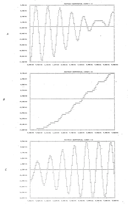
Example ( 1 ; F) Rossby Wave

The initial conditions f o r the f i r s t example are chosen as follows:

0 = cos(2nx/L) ; u = 0 ; v = 0 , (ICNUM-2)

i . e . . there is a wavenumber one geopotential disturbance, and the wind is in

geostrophic balance w i t h it. The main component o f this initial field (ICNUM=2)

is a Rossby wave. There are also small gravity wave components, since the

conditisns are nondivergent. In figure l a we show a plot o f height against x

and t (a so-called Hovm6ller diagram). The westward movement o f troughs .and

ridges is clear. The corresponding solution f o r the same initial conditions b u t

-1

.

with a mean zonal wind f i = 100m/s is shown in figure l b . The advective

e f f e c t o f the mean flow is clear. You may like t o check the phase-speed o f

the solution against t h e theoretical Rossby phase speed (see the equation

-1 -1

following (8): f = 1.~-04s": j3= l.E-11 m s ; k = 2 a / L , C = l.E+07 m;

4

= 1 .E+OSm2s-2). A three-dimensional plot of the Rossby wave solution ( f o r

G=O) is shown on the t i t l e page: note the high frequency ripples running along

the ridge; these are due t o the interference of the small amplitude gravity

wave components present in the initial condit.ions.

Example (2): Timesceles o f the Solutions

The value o f the geopotential a t a central point o f the grid.

resulting f r o m several d i f f e r e n t initial conditions, is plotted against time in

figure 2. The initial conditions are;

(2a) 0 = c o s ( b x / L ) ; u = 0 ; v = 0 (ICNUM=I

(2b) b = cos(2nx/L) ; u = 0 ; v = Ox (ICNUM=2)

(2c) B = c o s ( 2 n x / L ) ; u = 0 ; v = O (ICNUM=3)

These initial conditions may be described as follows: (28) represents a mixture

o f t w o gravity-inertia waves and a Rossby wave (no component is obviously

dominant); (2b) is essentially a Rossby wave ( w i t h small

G-I

wave components);

(2c) represents an eastward travelling gravity-inertia wave.. The figure clearly

shows the d i f f e r e n t timescales o f the evolving geopotential f o r the differing

types o f motion. The rotational motion (2b) has a much slower evolution than

the motion containing large gravity-wave components. It i s the principal goal o f

the initialization process t o remove the large. high frequency oscillations which

arise from the presence o f unrealistically large gravity-inertia components in

the initial data used f o r numerical forecasts. (The changing amplitude o f the

geopotential. evident in figure 2a and 2c. is due t o interference between

d i f f e r e n t components; the t o t a l eddy energy o f the disturbances remains

[image:17.589.97.533.38.741.2]

Figure 2. Time evolution of the geopotential at a central point

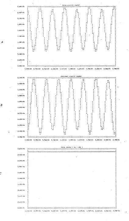
Example (3) : Conservation o f Eddy Energy

When the mean zonal wind vanishes, there is no physical source uf energy which might enable a disturbance t o grow with time: the t o t a l eddy energy remains constant (see equation ( 1 1 ) ) . We have n o t made any e f f o r t t o

ensure t h a t the numerical scheme reflects this conservation property; however, if the model is t o be o f any use f o r simulating atmospheric phenomena, the energy budget must be properly represented. In this example we s t a r t from initial conditions (2c) above (ICNUM=3) and calculate the eddy kinetic, available potential and t o t a l energy a t each timestep. Plots o f these as functions o f time are shown in figure 3. These clearly show how the energy may flow back and f o r t h between the kinetic and potential forms. due t o interaction between different wave components, Figure 3c demonstrates t h e conservation o f t o t a l eddy energy. (N.B. The Pdams Bashforth scheme is

marginally unstable; if an extended integration is carried out the energy will eventually begin t o grow in an unacceptable way; you may like t o t r y this, and

then rerun with a shorter timestep)

Example (4) : Wave

-

Mean Flow Interaction

[image:19.589.121.545.40.761.2]

Figure 3. Eddy energy for the initial conditions ICNUM = 3

(a) Kinetic energy ( b ) Available potential energy

C ( I * " , S I I Y I rwl" *E.* I" t o o . L * " C I

*.111..,

...

' ...

...

..

. . .

...,.

...

...

..

..

. . . .

. . . .

..

..

. . . .

. . .

. . .

. . . .

1 . 1 1 1 - 0 ,

-

. . .

. . . .

,

. . .

,

,

. . . .

. . .

[image:20.591.114.559.37.797.2]

. . .

,

...

...

. . .

1

,..n-0, -

. . .

. . .

. . .

. . .

. . .

. . .

,

. <

,

. . .

. . .

. . .

. . .

. . .

...

,

,

. . .

z..,c-o,

.

,

. . .

. . .

. . . . . .

. . .

,

..

.

,

. . .

. . .

. . . ,

,

. . .

. . .

. . .

. . .

,

I.--.,

- . . .

,

. . .

. . .

. . .

,

,

. . .

. . .

,

1

. . .

. . .

,

-a...I-.I

...

-

...

'

. . . . . .

. . .

. . .

,

B

,

,

. . . . . .

. . .

. . .

,

,

-1.1 le-.l

. . .

. . .

I

. . . . . .

. . .

. . .

,

. . .

. . .

,

. . .

. . .

. . .

.I..X.l,

. . .

,

. . .

. . .

. . .

. . .

. . .

,

3

. . .

. . .

. . .

. . .

,

I

. . : . . .

. . .

,

4.. %..,

. . .

. . . .

. . .

. . .

. . .

...

I

. . . .

...

. .a .

,

. . . .

. . .

...

. . . .

,

. . . .

. . . .

-%211-.1

-

...

...

. . . .

. . . .

. .

..

.

.

..

. . . .

.

,

...

' ...

...,...,...,...,...,...

* . I Y r . " o I . , , C.", ,.22r.o, I . I Y . 0 ,

...

r e . " , ,.,L.#, &.&,I.., 7 . 9 .2..T...I l.l,r+ll

Figure 4 . _{Eddy energy i n t h e presence o f a zonal flow (UBAR} = 100 m/s)

(a) Total eddy energy (b) Source term i n EQN ( 1 1 )

it would appear that this model is capable o f simulating more

complicated interactions between the mean flow and the eddy motions. No

further consideration of this matter is presented here. More specifically, the

question o f hydrodynamic instability o f the eddy motion has not been addressed.

and is l e f t f o r your considoration.

Suqqestions f o r Further 8DD/i~ati0n~

There follows a hastily assembled list of suggestions f o r making use

o f the model OYNRMO. I would be grateful t o hear o f your experiences with any

new tests, or any bugs found, etc.

First some trivial runs t o gain familiarity:

( 1 ) : Run the model with various initial conditions (ICNUM) t o produce the Rossby and Gravity-inertia waves before your verbeyes.

(2): Switch on IHOV t o generate Hovmbller diagrams f o r these.

( 3 ) : Run with various values o f A t t o illustrate computational instability when

the CFL criterion is violated.

(4): Run f o r extended period t o illustrate the ultimate breakdown due t o the

marginal instability o f the Rdams-Bashforth scheme; cure this by

reducing the timestep.

More Rdvanced Rpplications:

(1): Change the timestepping scheme. e.g. use Euler forward (unstablel),

Euler backward or Matsuno. Leapfrog. Trapemidal (implicit); these

are all discussed in Mesinger and Rrakawa (1976).

(2): Split the integration and use a semi-Lagrangian scheme f o r advection

(Bates and McDonald, 1982).

(3) Perform extended runs (perhaps with leapfrog scheme) t o check f o r

non-linear instability; see if this can be cured by reformulating the

finite differencing of the advection terms. Does non-linear instability

occur with a semi-Lagrangian scheme?

(4): Modify the model t o use either the primitive equations or the filtered

the t w o methods.

(5): Derive the equation expressing Conservation o f Potential Vorticity;

calculate this quantity numerically and see if the model is conserving

it properly.

(6): It is easy t o incorporate mountahs into the model. What s o r t of motion

is forced by orography? How does it e f f e c t the energy balance o f

the eddy motion? Note the very different response f o r small and

large mean flow.

(7):

Extend the model t o predict the mean flow. Calculate the energetics o f

the mean flow and investigate the phenomenon of vacillation (this Is

an essentially non-linear phenomenon, and there is no simple analytical

description of it 1.

(0): Investigate the possibilities f o r hydrodynamic instability of the eddy motion

in the presence of a non-zero zonal mean flow. What are the

energetics of the instability? What (if any) is i t s geophysical

relevance?

In doing any of the above experiments, do not be afraid t o make

even major changes t o the model code. Clean copies of the original code are

there f o r the asking (e.9. you can send me a request using the MAIL facility

on the DEC 20-50).

APPENDIX A: THE FILTERED EOURTIONS

The quasi-geostrophic approximation t o the shallow water equations is

derived here ( f o r more details see Haltiner and Williams, chapter 3 ) . Equations

(5). (6) and (7) are nondimensionalimd as in section 5 but with an advective

derivativ-s multiplied by Ro. Since the divergence is small compared t o the

vorticity we separate t h e wind into rotational and divergent p a r t s

V-?r)+VI ; V + = k x V J I ; VI=Vx

and ignore the l a t t e r where i t appears undifferentiated. We now assume t h a t

Ro a 1.

~~5

1 and RF 1, and drop ail terms which are o f order Ro o r smaller.

The resulting equations may be w r i t t e n (in dimensional form):

Note t h a t the divergence equation has become a diagnostic equation (i.e. it has

no time derivative): it shows t h a t the vorticity is geostrophic and gives the

rotational wind:

JI

= 0'/f ; v =

II,

= O ' J j (A41

Equations ( A l l . (A21 and (A31 are the quasi-geostrophic equations f o r our

one-dimensional model; although 161

l(1

the divergence terms in ( A l l and (A33

are o f t h e same magnitude as t h e other terms.

The equations ( A l l and (A31 can be used t o forecast the vorticity

and geopotential. Alternatively, we can eliminate 6 between them and get the

quasi-geostrophic potential vorticity equation :

With the use o f (R2) and (A41 this can be w r i t t e n in t e r m s o f 0' alone. R

diagnostic equation f o r t h e divergence is obtained by eliminating the time

derivatives between (A1 and (A3):

6~

-

(f2/8)6 = (,9/8) Ox + (G) Oux (A61

This is t h e quasi-geostrophic divergence equation and relates the divergence t o

The system

( A l l .

(A3) and (A61 are sometimes called the Filtered

Equations: they allow only the slow quasigeostrophic motion; the f a s t gravity

inertia modes are filtered out; you may check this by deriving the linear normal

mode solutions o f these equations and comparing the results with those (in

section 3) f o r the primitive equations. The model DYNAMO may easily be modified

t o use the filtered equations. The LOGICRL variable IOG should be used t o switch

from one system t o the other. R routine HELMID. analogous t o POlSlD but for

a Helmholtz equation, will have t o be written. You could, f o r example, t r y a

successive overrelaxation (SOR) method; l e t me know how you get on.

APPENDIX B: SOLUTION OF POISSON'S EOURTION.

After each forward step the new values of the velocities u end v

must be derived from the vorticity ( and divergence 6. If we solve two Poisson

equations f o r the stream-function

9

and velocity potential 1:

v29

= ( V l 2 = 6 (01

the velocities can be obtained by differentiation:

V =

k X V g

+

V x

(82)

In the present case we assume that the dependent variables are

independent o f y, are specified on the discrete grid Ix,,=O.x,.x,,

.,.

,x,,tCI. and

are periodic in x. Thus we must solve t w o equations of the form

d$/dx' = p ; $(O)=+(L) (03)

Since the reference potential is arbitrary we can choose +(0)=0. The discrete

equations (taking Ax=l) can then be written

-

0

,

-

20,

-

Pel

01 +

,

0

= P*

resulting equations added up t o obtain

.. .

this gives US ),; the f i r s t o f (84) then gives

IP2,

the second

0,.

and so f o r t h

until the f u l l solution is obtained. The value o f $,,. which should be zero. can be

used t o check t h e e f f e c t s o f roundoff e r r o r . The entire algorithm i s coded in

the procedure POISID. When the stream-function and velocity potential have

been derived the velocities on t h e staggered grid are obtained f r o m the

equations

u,, =

(xn

-

xn-,)/Ax ; vn = (+,,

-

$,,-,)/Ax

by calling the procedure 00x8. (The method o f solution described here was

found in Hockney and Eastwood. 1981

.

References

Bates. J.R. and R. McDonald. 1982: Multiply-upstream semi-Lagrangian advective

schemes: analysis and application t o a multi-level primitive equation

model. Mon. Weather Rev.

,

110, 1831-1842.

Haltiner. G. J. and R.T. Williams. 1980: Numerical Prediction and Dynamic

Meteorology. John Wiley 8 Sons. New York. 477pp.

Hockney. R.W. and J.W Eastwood. 1981: Computer Simulation Using Particles.

McGraw-Hill Inc.. New York, 540pp.

Holton. J.R., 1972: An Introduction t o Dynamic Meteorology. Academic Press,

New York, 319pp.

Holton, J.R. and C. Mass. 1976: Stratospheric vacillation cycles.

J.

Rtmos.

Sci. , 33, 2218-2225.

Mesinger. F. and A. Rrakawa. 1976: Numerical Methods Used in Rtmospheric

Models. WMO. GRRP Publication Series, No. 17.. Vol. 1.

Pedlosky, J., 1979: Geophysical

Fluid

Dynamics. Springer-Verieg, New York.

" D Y N A M O ' * . . . . . * * . * . l t . . . . . . . t * * . " . . . . . . t -t * * * . * . . . * . * * * * * " " " . ~ , , ,

S T A R T I N G FROM THE SHALLOW WATER E O U A T l O N S , THE V O R T l C l T Y AND D I V E R G E N C E E O U A T I O N S A R t D E Y I V E D . T H E B E T A E F F E C T THUS A P P E A R S E X P L I C I T L Y AN0 SO A L L FURTHER Y-DEPENDENCE O F THC P L R T U Y B A T I O N Q U A N T I T I E S CAN B E SUPRESSED. THE R E S U L T I S A S E T O F THREE E Q U A T I O N S W I T H TMO I N D E P E N D E N T V A R I A B L E S , X AND 1, AND THREE DEPENDENT V A R I A B L E S , TO H I T ,

D V l D X = V O R T I C I T Y DU/DX i D I V E R G E N C E F I = G E O P O T E N T I A L .

P E R I O D I C BOUNDARY C O N D I T I O N S ARE S P E C I F I E D , I.E. O ( X + L X t T ) = O I X t T )

FOR A L L P E R T U R B I T I O N Q U A N T I T I E S Q.

I N l l I A L C O N D I T I O N S ARE S E T BY S P E C I F Y I N G THE V A L U E S O F U l X t O l , V ( X ~ O ) I F I ( X r O l . FROM THESE THE I N I T I A L V A L U E S O F V O R T I C I T Y AND D I V E R G E N C E ARE I M M E D I A T E L Y D E R I V E D . A F T E R EACH FORWARD S T E P WE MUST S O L V E THO P O I S S O N E Q U A T I O N S ( W I T H P E R I O D I C B.C.3.)

L A P ( P S I 1 = V O R T I C I T Y L A P C C H I ) = D I V E R G t N C E . FROM THESE WE GET THE NEW V E L O C I T I E S I

U r O ( C H l ) l D r V 2 D I P S I I I D X .

T H E S P A T I A L G R I D I S STAGGERED1 THE V O R T l C l T Y AND D I V E R G E N C E A R E S P E C I F I E D AT "WHOLE P O I N T S * , A S I S THE G E O P O T E N T I A L l THE V E L O C I T I E S ARE AT ' H A L F POINTS'. V E L O C I T I E S NEEDED AT WHOLE P O I N T S ARE GOT BY AVERAGING. THE T I M E - S T E P P I N G I S DONE BY L N ADAMS-BASHFORTH S C H E M t t T H I S MEANS THAT WE NEED THE F O R C I N G 1R.H.S.) TERMS A T THO T I M E - L E V E L S .

"

I N C L U D E '.DYNAMO.COM' C

[---.---.-.----.--.---

C OPEN CONTROL (CARD) F I L E AND OUTPUT ( L I N E P R I N T E R ) F I L E

O P E N ( U N I T = S r D E V ~ C E ~ ' 0 S K K ~ A C C E S S = ' S E O I N \

X M O D E = ' A S C I I ,FILE='LIYNAMO.CDS')

O P E N ( U N I T = b r D E V I C E = ' D S K ' ~ A C C E S S = ' S E Q O U T ' t

X M O D E 1 ' A S C I I ' ~ F I L E = ' U Y N A M O . L P T ' )

C

C S E T U P THE I N I T I A L C O N D I T I O N S C A L L I C S

-

L

C C A L L THE I N l T I A L l Z A l I O N PROCEDURE

C I F ( I N I T ) C A L L L A P I N I NOT I M P L I M L N T E D I N T H I S VSN. C

-

C PERFORM THE I N T E G R A T I O N DO 1 0 0 0 NS;lrNSTEPS

N S T E P = NS

C L L L S T E P O N ( N S T E P ) LOO0 C O N T I N U E

P

C P R I N T OUT THE F I N A L R E S U L T S C A L L OUTPUT

C

t D E F I N E CONSTANTS A N 0 PARAMETERS AND S E T U P THE C GRID. I N I T I A L I Z E FLOW CONTROL V A R I A B L E S FOR THE RUN

C

I N C L U D E '0YNAMO.COM' DOUBLE P R E C I S I O N S T R I N G

r

"

C SONE PARAMETERS

DATA P 1 1 3 . 1 4 1 5 9 2 6 5 I r FCORll.E-04/rBETA/1.bE-ll/~GRAV/9.8LI

C SOME S C A L E S

DATA S X L / l r E t O b / r S X V / l O . /

c

S X T : I . I F C O R 1 T I M E S C A L E

S X D V = S X V I S X L I S C A L E FOR D I V E R G E N C E AND V O R T I C I T Y S X F I ; S X L ' S X V I S X T 1 S C A L E FOR GEOPOTENTIAL

c

C R E A D CONTROL PARAMETERS FOR THE FLOW O F C O M P U T A T I O N S R E A D I S . * ) STRING~LINEAR

READIS,*) STRING.IQG R E A O I S r * I S T R I N G I I N I T R E A D I S , * ) S T R I N G t I P R I N T R E h D l S r * ) STRINCINPRXNT

W R I T E ( b t 9 0 0 ) L I N E A A ~ I O G ~ I N I T I I P R I N T T N P R I N T

9 0 0 F O R M A T ( / ' DYNAMO 'I' RUN CONTROL PARAMETERS ' /

X ' L I N E A R ' r L l r ' OG ' , L I r ' I N I T ' , L l r ' I P R I N T ' r L 1 1 X ' P R I N T OUT I N T E R M E D I A T E R E S U L T S EVERY ' r 1 5 r ' S T E P S ' / )

P

.,

C S E T UP THE I N D E P E N O E N T V A R I A B L E D I S C R E T I Z A T I O N

R E A D I 5 r t ) S T R I N G P N X I NUMBER O F P O I N T S I N X - D I R E C T I O N R E A D I S , * ) STRINGIDK 1 G R I D L E N G T H I N X - D I R E C T I O N ( M E T R E S ) R E A O ( S r * l STRINGINSTEPS 1 NUMBER OF T I M E S T E P S FOR RUN READ(S,*) STRINCIDT 1 T I M E I N C R E M E N T (SECONDS)

L E N X s X L E N 1 1 0 0 0 . 1 CHANNEL L E N G T H I N KM. T L E N N S T E P S t D T

H L E N TLEN/(bO..bO.) 1 FORECAST L E N G T H I N HOURS W R 1 T E ( b , 9 0 1 ) N X I L E N X I D X ~ N S T E P S I H L E N r D T

TYPE 9 0 1 , NX,LENX,DX,NSTEPS,HLEN,PT

9 0 1 F O R M A T I ' G R l O P T S t ' r I 4 r 3 X 1 X ' CHANNEL LENGTH8 ..lb,'KM', X ' G R I O L E N G T H OX: ',-3PFb.O.'KM'/ K ' TIMESTEPS% ' , ~ V , S X ,

X ', FORECAST L E N G T H I ' r O P F S . l , ' HOURS ',

x ' T I M E S I E P : ',OPFb.O,' S E c . ' I l

C CALCULATE THE INDEPENDENT V A R I A B L E S (FOR PLOT AXES) DO 1 0 NN=O,NXPl

X I N N ) = N N * O X I l . E + 0 3 : G R I O P O I N T S (KM) 1 0 CON1 I N U E

DO 2 0 NN=O,NSTEPS

T ( N N ) = N N * O T / ( b 0 . + 6 0 . ) 1 T I M S T E P S (HUUHS)

2 0 CONTINUE

C READ M E I N F ~ o d PARAMETERS REAO(5r.) S I R I N G I J H A R R E A O ( 5 r t ) S T R I ~ G I F I ~ A R UO = U B A R I S X V

F I O = F I B A R I S X F I

,-

"

RO = S X V / I F C O R + S X L ) 1 ROSSBY NUMBER 1 0 0

RB r BETA.SXL/FCOR 1 MEASURE OF BETA E F F E C T C

R F = F I B A R I ( F C O R * S X L ) + t 2 1 RECIPROCAL OF FROUOE NO. C

P

.

W R I T E ( b r 9 0 1 ) UBARIFIBAR,AOIRR,RF

9 0 7 FORMAT(! MEAN ZONAL WIND UBAR = ',Fb.O,' M I S ' /

X + MEAN CEOPOTENTIALI',FB.O,' I M I s I * * ~ 'I

X ' R A T I O RB : ' , l P E I O . l / X R A T I O R F I ' t l P E 1 O . I I ) C

c READ I N D I C A T O R FOR I N I T I A L C O N O l l l O N S R E A O ( 5 r * ) S T R I N G , I C N U M

TYPE 9 9 0 1 , l C N U M U R I T E ( 4 r 9 9 0 1 ) I C N U M

9 9 0 1 FORMAT(' I N I T l A L CONOIT1ONS: I C S = * , I 2 / )

,-

"

C READ I N O I C A T U H S FOR HOVMOELLER DIAGRAMS READIS,*) S T R I N G , IHOV~NXHOVINTHOV TYPE P ~ O ~ , I H O V I N X H O V I N T H O V

N R l T E l b r 9 9 0 2 ) IHOVINXHOV,NTHOV

9 9 0 2 FORMAT(' HOVMOELLER DIAGRAMS ' , L 2 , 2 1 4 / )

C C

RETURN C

END 1 0 3

[---

SUBROUTINE I C S

C c

C D E F I N E THE I N I T I A L C O N D I T I O N S . THE VALUES S P E C I F I E D ARE C

C FOR U I VI AN0 F 1 : ' T H E I N I T I A L VALUES OF V E L O C I T Y ARE 1 0 4

C S P E C I F I E D AT H A L F P O I N T S ( S T A R T I N G AT I = - 1 1 2 ) : THE VALUES C OF F I ARE G I V E N AT WHOLE P O I N T S ( S T A R T I N G AT 1'0).

C C

I N C L U D E 'DYNAMO.COM'

REAL K O U N l I Z O ) r P H A S E ( 2 O ) r L H P L ( Z O ) REAL COSN ( O : Z O l ) , S l N N ( 0 : 2 0 1 ) PEAL COSNMHIOIZOl)rSINNMH(0:201)

C

NSTEP = 0

C D E F I N E THE l N l T I b L V E L O C I T I E S &NO G E O P f l T E N T l A L

C ~ t r . r SOME SAMPLE I.CS. AHE G I V E N HERE1 I F YUU WANT TO D E F I N E

C*.r*. OTHER C O N D I T I O N S r I D E N T I F Y THEM U S I N G ICNUM > 4. C

AM = 1. 1 ZONAL WAVENUMBER ONE F I A M P E 1 . E t 0 3

F I A M P = F I 4 M P I S X F I I NON-DIM AMPLITUDE OF GEOPOTENTIAL XNX r F L O A T C N X )

DO 1 0 0 NN=O,NXPI XNN a F L O A T ( N N ) XNMH = F L O A T I N N ) - 0 . 5 U I N N ) s 0 .

V I N N ) : 0. F I ( N N ) = 0.

COSN (NN) E C O S I A M * Z . * P l * X N N I X N X I COSNMHCNN) r C O S l A H + Z . * P I * X N M H I X N X ) S I N N I N N ) = S I N ( A M t 2 . t P I t X N N / X N X ) S I N N M H I N N ) r S I N ( A M * Z . * P I * X N M H / X N X ) CONTINUE

CALCULATE SOME PHASE-SPEEDS (SEE REPORT, S E C T I O N 3 ) XLEN r NX+IOX.SXL)

WLEN Z XLEN I AM

2 K = 2 . * P I I W L E N

CGRAV = S O R T 1 F I B A R t ( F C O R / Z K ) + + Z )

CROSB =

-

( B E T A / Z K * * Z ) / ( I . t ( F C O R ~ ~ Z / l F I B A R * L K I * 2 1 ) )

U R I T E ( b r 9 2 2 2 1 ) CGRAV,CROSB TYPE 9 2 2 2 1 , CGRAV,CROSB

F O R M A T I ' UAVESPEEDS: CGr CR

.

l P Z E I 2 . 3 / )

GO TO 1 1 0 1 ~ 1 0 2 ~ 1 0 3 ~ 1 0 4 ~ 1 0 5 ~ 1 0 b ~ 1 0 7 ~ 1 0 8 ) ~ 1 C N U M

STOP ' ICNUM O U T S I O E RANGE '

PURE G E O P O T E N T I A L PERTURBATION: C O M B I N A T I O N OF THREE WAVES. C A L L V L C C O N ( F I A M P , C O S N I F I I I , N Y P I ) $ GO TO 1 0 0 0

APPROX ROSSBY HAVE

CALL V ~ . C C O N ( F I A M P , C O S N , F I , O , N X P ~ )

C A L L ODXB(FI,V,NX,DX) i GO TO LOO0 APPROX EASTWARO-TRAVELLING 6 - 1 WAVE C A L L V E C C O N C F I A H P , C O S N r F I , O , N X P l )

uanp s FIAMP

C A L L V E C C O N ( U A M P I C O S N M H ~ U , O O N X P I ) I GO TO 1 0 0 0 APPROX WESTWARD-TRAVELLING G - I WAVE

C A L L V E C C O N ( F I A M P , C O S N I F I ~ O O N X P ~ ) UAMP =

-

F I A M P

C A L L VECCON(UAMP,COSNMH,U,O,NXPI) I GO TO 1 0 0 0 MORE ACCURATE ROSSBY WPVE

CONTINUE C = CROSB

UAMP = l C / F I H A R ) . F I A M P * ( S X F I / S X V )

VAMP I Z K * F C O R I ( Z K t t 2 * C t B E l A ) t IIAMP C A L L V E C C O N ( F I A M P I C O S N , F I ~ O ~ N X P L ) C A L L V E C C O N I U A ~ P . C O S N M H , U , O , N X P ~ ) C A L L V E C C O N C V A M P , S I N N M H r V , 0 o N X P l )

-

c MORE ACCURATE EASTWLRD G R A V I T Y WAVE

I O b C A L L V E C C O N ( F I A H P , C O S N , F ~ , O , N X P I ) C

C * CGRAV C CALCULATE THE I N I T I A L ENERGIES.

UAMP = (C/FIBAR)~FILMP.(SIFIISXVI C A L L ENERGY(NSTEP)

C A L L VECCON(UAMP.COSNWH,U,0,NXP1) i GO TO 1 0 0 0 C

r C S A V E FIELD V A L U E S A T A CENTRAL POINT FOR PLOTTING

.

C MORE ACCURATE WESTUARO G R A V I T Y WAVE NXH = N X I Z

1 0 7 C A L L V E C C O N ( F I A M P , C U S N , F I , Q , N X P ~ ) P T V ( N S T E P 1 P T U ( N S T E P ) = = ULHXH) V ( N x H ) P T F I ( N S T E P ) = F I C N X H ) C =

-

CGRAV

UAMP i ( C / F l B A R l * F I P L P ~ ( S X F I / s x V l P l D I V ( N S T E P ) D I V I N X H )

C A L L VECCON(UAMPlCOSNMH,U,O,NxP1) : GO TU 1 0 0 0 r

-

P T V O R T I N S T E P ) VORTCNXH)

c

C 1 0 8 CONTINUE I GO TO 1 0 0 0 C SAVE VALUES FOR THE HOVMOELLER DIAGRAM U R l T E ( 1 0 ) F I UF F 1 .

C L * ~ . n ~ . n n ~ ~ n # u ~ L X I . # # ~ ~ ~ # ~ # X n # u n n u n ~ n n n n R n n n n n n # u n n # u " u n " " u # n u n * C C C O M B I N A T I O N OF WAVES W I T H A M I N U S - F I V E - T H I R D S SPECTRUM

C AND 6EOSTROPHIC WIND ( I N I T I A L I Z A T I O N TEST) RETURN

LOB CONTINUE c---*---.---. END

F I A M P = l . E t 0 3

F I A M P = F I A M P / S X F I _C SUBROUTINE STEPON(NSTEP)

KMAX r 3 C PERFORM S I N G L E T I M E S T E P FOR DYNAMO

POWER = - ( 5 . / 3 . ) C

POWER = 0. I N C L U D E !DYNAMD.COM'

U R I T E ( b r 9 0 7 1 ) KMAXIPOWER C

9 0 7 1 F O R M A T ( / L ICNUM 8 KMAX: ' r 1 U r ' WAVES, PUWER SPECTRUM: .,F8.4/) C GET RHS OF V O R T I C I T Y , DIVERGENCE AND C O N T I N U I T Y EQUATIONS

DO 1 6 6 K K l l r K M A X C AT THE PRESENT T I H E L E V E L AND PUT I N R H S l V t R H S I D AND R H S I C

KOUNTCKK) = KK C (OLD V A L U E S ARE I N RHS2 I F NSTEP r 0 ) .

A M P L I K K I = F L U A l l K K ) + t P O W F R P

""..

.

...

".

C A L L P L D T L N ( K O U N T + A H P L . I r K M A X ~ O . , O . , . A W L .)

C C e L L P L O T L N ( K O U N T r P H A S E ~ I ~ K M A X ~ O . O O . ~ ' PHASE 'I

XNX = F L O A T ( N X 1 DO I 0 0 6 NNs0,NXPI

XNN I FLOATCNN) U (NN) = 0. V (NN) = 0. SUM rn 0.0

DO IOOOb KKz1,KMAX XKK S F L O A T C K K I

SUM S SUM AMPLCXKKI + COS(XKK*Z.*PI*XNN/XNX t PHASE(XKK) )

1 0 0 0 6 CONTINUE

F I ( N N ) = S U M I F I A M P 1 0 0 6 CONTINUE

C A L L DDXB(FIIVINX,OX)

CONTINUE i GO TO 1 0 0 0

~ ~ X ~ # I # n n n # # ~ # # N ~ n ~ # # ~ n # w i l n C # # # # n w u n n ~ # n u # u n u n ~ # # # n # ~ # # u n n # n # n # u n u n n u # u #

L

C*."..

c

1 0 0 0 CONTINUE

r

-

C CALCULATE DIVERGENCE AND V O R T l C l T Y ( A T WHOLE P O I N T S ) C A L L ODXF(U, OIVINXIDX)

C A L L D O X F ( V I V O R T ~ N X ~ O X )

c

C PLOT I N I T I A L VALUES OF DEPENDENT V A R I A R L E S

I F ( 1 P R I N T ) C A L L PLOTLN(X,U , O , N X I - Z . , ~ Z . ~ ' I N I T I A L U 'I

I F C I P R I N T I C A L L PLO1LNCX.V , O I N X I - Z . ~ + Z . ~ ' I N I ~ I A L V 'I

I F ( I P R I N 1 ) C A L L P L O T L N ( X , F I r O l N X ~ - Z . , + 2 . , ' I N I T I A L F I ' I C I F ( I P R I N 1 ) C A L L P L O T L N ( X I V O R T ~ O P N X , 0.. O.,'VORTICITY 'I

C I F ( I P R 1 N T ) C A L L P L O T L N [ X I O I V rO,NX# 0.. O.,'DIVERGENCE'I

XNL S 1.0 1 NON-LINEAR FACTOR

I F C L I N E A R I XNL i 0.0

c

C CALCULATE THE AOVECTION TERMS

C A L L X H E A N B ( V O R T I W D R K ~ ~ N X ) 1

C A L L XMEANB(D1V r W O R K 3 r N X ) 1 AVERAGE TO V E L O C I T Y P O I N T S C A L L X H E A N B I F I r W O R K 4 r N X ) 1

DO 1 0 0 NN=O,NXPI

C A L L D O I F l * O R K 2 , n D R K I , N X I D x ) I

C A L L D D X ~ l # O R K 3 , ~ O R ~ Z ~ N x . O X ) 1 A O r C C l l O h TERMS C A L L D 0 X F ( ~ 0 R K C , I U R ~ 3 , h X , ~ X 1 I

C A L L XMEANFIUIUINXI I U AND V NO LONGER NEEDED AT H A L F C A L L XMEANFIV,V,NX) I P O I N T S BUT AT WHOLE P O I N T S .

c

C A L L DDXX(FI,WORK4,NX,DX) I PRESSURE GRADIENT TERM C GET R.H.S. OF E O U L T I O N S ( I 8 ) r 1 1 9 ) . AND ( 2 0 )

D o 2 0 0 N N r 0 , N X P I

RHSIVINN) =

-

( RO=WORKIINN)+ DIV(NN)+RB*VINNI I

R H S I D ( N N 1

-

-

( R U * W O R K Z ( N N ) - V O R T ( N N I t R B B U ( N N ) t W O R K 4 ( N N ) 1

R H S I C ( N N 1 =

-

1 R O ~ ~ O R K 3 l N N ) - ~ O ~ U O ~ V ~ N N ~ t R F F D 1 V ( N N l ) 2 0 0

-

CONTINUE

L

C * * t

2 5 0 C

c

3 0 0

c c c C C C C C CCC CCC CCC c C C C C C C C C C C t

-.-

F N M I = -0.5

IF(NSTEP.GT.0) GO TO 2 5 0 F N a 1.0

F N M I = 0.0 1 F I R S T STEP I S EULER FORWARD CONTINUE

ACTUAL FORWARO STEP, E Q U A T I O N S ( 1 8 ) r ( 1 9 ) , ( 2 0 ) DO 3 0 0 N N = O r N X P I

N O R K I ( N U ) s VORT(NN) t D E L T ( F U * ~ H S I V ( N N ) t F N M I * R H S Z V ( N N ) I

WORKZCNN) = O I V ( N N ) t D E L T (FN*RHSlD(NN)tFNMl*HHS2D(NN))

WORKICNN) = F I C N N ) D E L T (FN*RHSIC(NN)tFNM1*RHSZC(NN))

CONTINUE

I F THE T I M E S T E P P I N G SCHEME I S TWO-LEVEL UC ONLY NEED TO KEEP THE MOST RECENT VALUES; I F I T I S A THKEE-LEVEL SCHEME (E.G. LEAPFROG OH AOAMS BASHFORTH) THEN SOME OLD Y l L l l F S W I L L BE NEEDED. I H E E M P H A S I S I N T H I S 1 - 0 MODEL

SAVE THE OLD VALUES AN0 RELOCATC THE UPOATED OhES C A L L M E M O V E ( V O R T ~ V O R O L D t O ~ N X P I 1 1

C A L L YEMOYE(DIV ~ D I Y O L D ~ O I N X P I I 1 NOT HEOUIRED T H I S VSh.

C A L L H E M O V E ( W O R K I , V O R T I O ~ N X P L ) !

C A L L MEMOVE(WORKZ,DIV ,O,NXPI) 1 MOVE I N NEW VALUES C A L L MtMOVE(WORK3,FI ,O,NXPI) 1

CALCULATE THE V E L O C I T I E S AT THE NEW T I M E

C A L L P O I S I D ( C H 1 , D I V r N X r D X ) I V E L O C I T Y P O T E N T I A L C A L L P O I S L D ( P S l r V O R T ~ N X ~ D X ) 1 STREAM F U N C T I O N CALL. DDXB(CHI,U,NX,DX) 1 ZONAL V E L O C I T Y C A L L D D X B ( P S I r V 8 N X , D X ) 1 M E R I D I O N A L V E L O C I T Y CALCULATE THE E N E R G E T I C S

C A L L ENERGY(NSTEP1

S H I F T R.H.9 TERMS FOR NEXT CYCLE C A L L M E M O V E ( R H S I V ~ R H S ~ V I O , N X P ~ ) C A L L M E M O V E ( R H S 1 D , R H S Z D , O r N X P I ) C A L L M E M O V E ( R t l S I C r R H S 2 C r 0 , N X P l l

SAVE F I E L D VALUES AT A CENTRLL P O I N T (FOR P L O T T I N G ) NXH s N X / 2

P T U ( N S T E P ) i U ( N X H )

P T V ( N S T E P ) n VCNXH) P T F I ( N 3 T E P ) = F I C N X H ) P T D I V ( N S 7 E P ) = D I V ( N X H ) P T V D R T ( N S T E P ) S VORT(NXH)

SAVE VALUES FOR THE HOVMOELLER DIAGRAM OF F I .

I F ( ( N S T E P / N T H O V ~ N T H O V ) . E O , N S T E P ) W R I T E ( 1 0 ) F I

RETURN

C N n

-

SUBROUTINE ENEKGY(NSTEP)

C

C CALCULATE THE ZONALLY AVERAGE0 E N E R G I E S ( S E t REPOHTI SEC 4 )

.-

b

I N C L U D E *DYNAMO.COM' C

XK n S X V t * 2 * S X F I / l Z . * G R 4 V ) XA = S X F I * + Z / ( Z . * G R A V ) XNX 3 NX

ROTKE = 0 .

D I V K E 1 0.

AVPE = 0.

sn,,!4r ; 0 .

-

-

-

. .

-

.

.

0 0 1 0 0 N N Z l r N X

ROTKE r ROTKE + IV(NN)tr2)+(FIO+(FI(NN-I)+FI(NN))/Z)*XK

D l V K E = D ~ V K E + (U(NN).*Z)*(FIOt(FI(NN-L)+FI(NN))/Z1lXK

AVPE : AVPE t ( F I ( N N ) * * 2 ) * X A

SOURC = SOURC t ( V ( N N ) t 0 . 5 * ( U ( N N ) * * 2 * V ( H N ) * . Z ) * S X V * * 3

X t V(NN)~(FI(NN-~)+FI(NN))/Z*SXV*SXFI )

1 0 0 CONTINUE

EDDYKE E R O T K E t D l V K E EOyTOT = EOOYKE AVPE

KEROT(NSTEP) = ( L / X N X ) * R O T K E 1 ROTATIONAL KINETIC ENERGY K E D I V ( N S T E P ) I ( I / X N X ) * D I V K E 1 DIVERGENT K I N E T I C ENERGY

C

C CALCULATE RATE OF CHANGE OF EDDY ENERGY 8 Y F I N I T E D I F F E R E N C E I F ( N S T E P . G T . ~ )

x D D T A P K ( N S T E P ) = ( A P L U S K ( N S T E P I - A P L U ~ K ( N S T E P - ~ ) ) / ( D T * S X T )

C

C P R I N T / T i P E THE ENERGIES AT L I C M T I H E S T E P : l h E Y G I V E A GOOD C I N D I C A T I O N OF NUMERICAL S T A d l L I T Y OR I N S T A L I L I T V

r

-

- P I I F 1 0 . 9 9 9 0 1 1 ...,..-.-... ~ s T E P , R o T K E , D I v x E , E ~ D Y K E , A ~ P E , E ~ ~ T ~ T , S O U R C

T Y P E 9 9 9 0 1 , N S T E P , R O T U E , D ~ V K E , E D D Y K E ~

9 9 9 0 1 FORMAT(* NSTEP: ' , I U r V KR,KO,KTrAP,

-

C

RETURN

c

C P R I N T OUT THE RESULTS OF THE RUN

c

INCLUDE 'DYNAMO.COM' C

C A L C j L A I l O h OF V A R I O U S F l h l T E O I F F E U E h C E S ( 1 ) CEhTRED F I R S T D I F f E R E h C E

C PLOT THE F I E L O VALUES AT THE M I D D L E P O I N T

Y D I Y F ( L . O O O O > >

. . .

,

-

.

-

, ,

. .

.

-

,

9 9 9 9 2 FORMAT(/.. * * . . + r + * . * P O I N T TENOENCIES t.tt.*.t**./) I F C I P R I N T ) C A L L P L O I L N ( T , P T U ~ O I Y S T E P S , O O . , O O . ~ ' M I D P T I1 ' ) I F C I P R I N T ) C A L L P L O T L N ( T r P T V rO~NSTEPS,OO.roO.r'MIOPT v ' 1

I F ( I P R I N 1 ) C A L L P L O T L N ( T . P T F 1 ,O.NSTEPS,OO.,OO..'MIDPT F 1 C I F ( 1 P R I N T ) C A L L P L O T L N ( T , P T D I V ~ O , N S T E P S I O O . , O O . . ' ~ I O P T O I V * )

C I F ( 1 P R I N T ) C A L L P L D T L N ( T ~ P T V O R T ~ O ~ N S T E P S S O O O O O O O t ' H I D P T VORT')

"

RETURN ( 2 ) FORNARD F I R S T OIFFERENCE

ENTRY D D X F ( F , O I F F , N r D E L T A ) DO 2 0 N N Z l r N

D I F F C N N ) ; ( F ( N N t 1 ) - F ( N N ) I / D E L T A

-

C GRAPH THE E V O L U T I O N OF THE ENERGY Q U A N T I T I E S W R I T E ( O , 9 9 9 9 3 )

9 9 9 9 3 F O R H A T ( I ' .****+*-+* ENERGY Q U A N T I T I E S .t.++.rr.r./) I F ( I P R I N T 1 C A L L P L D T L N ( T , K E R O T , O , I + S T E P S , O., I.,' ROT KE .I

I F ( 1 P R I N T ) C A L L P L O T L N ~ T ~ K E D I V I O ~ N S T E P J ~ 0.. I.,' D I V KE 'I

I F ( 1 P R I N T ) C A L L P L O T L N ( T I K E T O T ~ O I N S T E P S ~ O., I . , ' TOT SE * )

I F ( I P R I N 1 ) C A L L P L O T L N ( T , APE r O , N S l E P S , 0.. I.,' APE ' 1 I F ( 1 P R I N T ) C A L L P L O T L N ( T ~ A P L U 3 K v O r N S T C P S s 0 . . I . , ' APLUSK ' ) I F ( 1 P R I N T ) C A L L PLDTLN(T,SOURCE,O,NSTEPS, 0,. O.,' SOURCE ' )

I F ( 1 P R I N T ) C A L L P L O T L N ( T I O O T A P K , O , N S T E P S , 0.. O.,' DOTbPK

r

CONTINUE

C A L L E N D S ( D I F F p N 1 RETURN

( 3 ) BACKWARD F I R S T D I F F E R E N C E ENTRY DDXB(F,DIFFINIOELTA)

DO 30 N N = I , N

D I F F C N N ) E ( F ( N N ) - F ( N N - I ) / OELTA CONTINUE

C A L L E N D S ( D I F F , N ) RETURN

( 4 ) C E N T R E D SECOND OIFFERENCE ENTRY O D X X ( F I D I F F , N t D E L T A )

C PLOT HOVMOELLER DIAGRAM OF GEOPOTENTIAL I F ( I H D V ) C A L L HOVMOL

r

RETURN END

c---.---.---

SUBROUTINE P O I S I O ( P H I r R H O I N ~ O E L T A )

r

DO 4 0 N N z l r N

O I F F ( N N ) ( F ( N N + ~ ) ~ F ( N N - ~ ) - Z . . F ( N N ) ) / ( D E L T A * * ~ )

CONTINUE

C A L L ENDS(DIFF,N) RETURN

-

C SOLVE A P O I S S O N E Q U A T I O N I N ONE D I M E N S I O N

c ' NITH PERIODIC BOUNDARY CONDITIONS

END

AVERAGING OPERATORS (FORWARD AND BACK#ARD) SUBROUTINE X M E A N F ( F , F B L R X t N )

D I M E N S I O N F ( O : N l , F B A R X ( O : N ) DO 1 0 N N r l , N

F B A R X ( N N I = ( F ( N N ) t F ( N N t l ) 1 / 2.0

C L A P ( P H 1 ) = RHO

C WMERE L A P I S THE L A P L A C I A N OPERATOR

C I R E F : HOCKNEY, R.W. AND J.W. EASTWOOD, 19.51: C 'COMPUTER S I M U L A T I O N U S I N G P A R T I C L E S " C HC G R A H - H I L L INC., NEW YORKr 5UOPP.1

"

-

R E A L PHI(O:N),RHO(OIN) C

C ASSUME THE END VALUES V A N I S H (THEY ARE A R B I T R A R Y ) . P H I ( 0 ) = 0 .

C CALCULATE THE F I R S T VALUE DECSO = O E L T A h * 2

SUM i 0.0

CONTINUE

C A L L ENDS(FBARX,N) RETURN

E N T R Y XMEANB(F,FBARXIN) DO 2 0 NN.N.1,-I

F B A R X ( N N 1 i ( F ( N N - l l t F ( N N ) ) 2.0 CONTINUE

C A L L ENDS(FUARXIN) RETURN

DO 1 0 0 N N r l r N

SUM = SUM t N N I R H O f N N ) 1 0 0 r O N T 1 N U F

END

PHI(I)-; ( S U M / N ) * o E L S Q

C LOOP FOR THE OTHER VALUES _{SUBROUTINE E N D S C A r N )}

F I L L END VALUES OF A P E R I O D I C AURA* REAL A ( O I N 1

. l o ) = * I N ) DO 2 0 0 NNZ2,N

P H I ( N N ) = RHO(NN-l).DELSBt2.tPHI(NN-l)-PHI(NN-2)

2 0 0 CONTINUE

C _{A ~ N + I ) = - A ( ! )}

WOO

IYI0

C

0

a

o

<

W

0

J

lll

O:

.

...

NNN

NNN

0-

0

P

0

z.

^Y

-

-W

<N--3N--a

1

IIZl1SSZ

C>PP">PP..

LL-.ac-<<c

W

aaz

aaz

~YIYYOOUUO

SUBROUTINE HOVMOL

P R I N T OUT A HOVMOELLER D I A G R A M FROM THE VALUES STORED ON F I L E 1 0

D I M E N S I O N -CHAR(~I)

DATA CHAR /,O,,. .,'l,,' .,'2.,, , , ' 3 ' , ' ','4',' ' , ' 5 * ,

x

.

.,.b',' * , . 7 . , , . , , B , , ' . , . 9 . , . ','0'/ NXPTS : N X P I / N X H O V

I F ( N X P T S . G l . 1 2 1 ) RETURN, CLOSE ( U N I T z I O )

O P E N ( U N I T ~ l O , O E V I C E ~ ' S C R H , l C C E S s = ' s E O 1 ~ ~ ,

DO 1 0 0 0 NSTEP = OPNSTEPSINTHOV R E A D ( I O 1 F I

IF(NSTEP.GT.0) GO TO 2 0 0 D E F I N E ZERO AND S P A C I N G ZWAX 8 A B S ( F I I 0 ) ) DO 1 0 0 NNal.NX.NXHOV

A B S F l = A B S ( F I ( N N ~ )

I F ( Z n A X . L T . A B S F 1 ) Z H A X = A B S F I CONTINUE

ZERO i 0.

.

C D E R I V E P R I N T CHARACTERS FOR THE ROW 2 0 0 CONTINUE

DO 4 0 0 NN=O,NXPl,NXHOV F I N N r F I I N N )

I N 0 = MOO(INT((F1NN-ZERO)/SPACEt2OOO.l,2oltl

Z E 0 R A ( N N ) :I S H A R ( I N 0 )

4 0 0 CONTINUE

C

C P R I N T THE RON OF CHARACTERS

W R I T E ( b r P 9 9 1 N S T E P , l Z E B R A ( N N ) . N N = O , N X P T S l TYPE 9 9 9 , N S T E P ~ l Z E B R A ( N N ) r N N = o , N X P T S l

999 . F O R M A T l I X ~ I b r 4 X ~ I 2 l A l )

?

.

1 0 0 0 CONTINUE

~ R I T < ~ ~ , P ~ ~ O I I C

c---

C ~0YNAMO.COM'

C' COMMON BLOCKS FOR OYNAMO C

C SET MAXIMUM D I M E N S I O N S FOR ARFAYS PARAMETER N P Y = Z O l , N P T = 4 0 0 1

-

L

C PARAMETERS CONTKOLING THE FLOW UF C A L C U L A T I O N S L O G I C A L L l N E A R , I O G , l N I T , l P R I N T , I H O V

I N T E G E R N P R I N T , ICNUM, NXHOV,NTHOV

COMMON / F L O N / L I N E A R , I O G r l N I T , I P R I N T ~ N P R I N T , ICNUM, C

C VARIOUS CONSTANTS, PARAMETERS AN0 SCALES

CUMMON / P A R A M S / PI, F C O R , B E T A , UIAR,UO,FIBAR,FIO, RF.RO,RU.

X GRAVI SXL,SXT,SXV,SXDV,SXFI

C

C INDEPLNOENT V A R I A B L E S , INCREMENTS, GRlDSPECS, ETC. REAL X ( O 1 N P X ) , T ( O t N P T )

C O M W N / I V A R S / N X , N X P ~ , N S T E P S I D X I O T I Y I T

C

C DEPENDENT V A R I A B L E S (TWO T I M E L E V E L S ) , H O R I Z O N T A L V E L O C l T l E S t C GEOPOTENTIAL, V O R T I C I T Y AND DIVERGENCE.

R E A L U ( 0 : N P X ) r V (OZNPX)

REAL F I ( O I N P X I r V O R T 1 O : N P X ) r D I V ( 0 : N P X I C R E A L F I O L D - - - l O : N P X ) ~ V O R O L D ~ O : N P X ) t D 1 V O L D ( O : N P X )

COMMON /OVARS/ U I V ~ F I ~ V O R T , D I V

C X F l O L O ,VOROLDIDIVOLD I NOT REQD T H I S VSN C

C ' STREAM F U N C T I O N AND V E L O C I T Y P O T E N T I A L REAL P S I l O : N P X l r C H I ( O : N P X )

COMMON / P S I C H I / P S I t C H I C

C R I G H T HAND S I D E S ( A T TUO T I M E S )

R E A L Y H S I V I O : N P X ) , R H S I O ( O : N P ~ I , H H S I C ~ O : N P X )

REAL R H S ~ V ( O : N P X ) ~ R H S E D ( O : N P X ) ~ R H S ~ C ( O : N P X I COMMON /RHS/ R H S I V . R H S I O , R H S I C , H H S Z V V R H S ~ D D H H S ~ C

C

-

C P O I N T VALUES OF OEPtNOENT V A R I A ~ L E S REAL P T U ( O : N P T ) ~ P T V ( O : ~ P T ) ~ P T F I ( O I N P f l REAL P T V O R T ( O : N P T I r P T D I V ( O : N P f )

COMMON / P O I N T S / P T U I P T V , P T F I I P T V O R T ~ P T D ~ V

C

C W O R K ~ N G SPACE

REAL W 0 R K l ( 0 : N P X ) , W U R K 2 ( 0 : N P X ~ ~ W