PROJECTIONS OR DEAD-ZONES: A NON-SINGULAR
PERFORMANCE COMPARISON IN ROBUST ADAPTIVE
CONTROL
Ahmad Sanei, Mark French
Department of Electronics and Computer ScienceUniversity of Southampton, U.K. as99r|mcf @ecs.soton.ac.uk
http://www.isis.ecs.soton.ac.uk/control
Keywords: Robust Adaptive control, Non-singular Perfor-mance.
Abstract
We consider robust adaptive control designs for relative degree one, minimum phase linear systems of known high frequency gain. The designs are based on the dead-zone and projection modifications, and we compare their performance w.r.t. a worst case transient cost functional penalising the L∞ norm of the output, control and control derivative. If a bound on the L∞ norm of the disturbance is known, it is shown that the dead-zone controller outperforms the projection controller when the a-priori information on the unknown system parameter is suffi-ciently conservative.
1
Introduction
It is well known that adaptive control is suitable for physical systems whose mathematical model contains an uncertain pa-rameterθ. A common feature of adaptive designs is the con-struction of a time varying parameter θˆwhose value is trolled by an adaptive law. In contrast with most adaptive con-trol mechanisms which would attempt to ‘identify’ or ‘esti-mate’ the uncertain parameter θof the plant, the objective of a ‘non-identifier-based’ adaptive controller is to use certain in-formation about the plant to find suitable methods of system regulation. In other words, the adaptive law has no interest to identify or estimate the unknown plant parameterθ, but merely attempts to seek out a stabilising value ofθˆ. See eg. [1, 6, 7, 9] and [3] for an overview.
However this method, like other adaptive controllers, is sus-ceptible to phenomena such as parameter drift even when small disturbances are present. To overcome such problems, a num-ber of standard techniques are widely utilised, such as dead-zones,σmodification, projection modification [8].
Each of these designs have advantages and drawbacks. For example, dead-zone modifications require a-priori knowledge of the disturbance level, and only achieve convergence of the output to some pre-specified neighbourhood of the origin (whilst keeping all signals bounded). In particular if the dis-turbance vanishes, then the dead-zone controller does not
typ-ically achieve convergence to zero, the convergence remains to the pre-specified neighbourhood of the origin. On the other hand, projection modifications generally achieve boundedness of all signals, and furthermore have the desirable property that if no disturbances are present, then the output converges to zero, however, an arbitrarily smallL∞disturbance can com-pletely destroy any convergence of the output.
This illustrates that in the case of asymptotic performance, there are some known characterisations of ‘good’ and ‘bad’ behaviour. However, there are many situations in which we cannot definitively state whether a projection or dead-zone con-troller is superior even when only considering asymptotic per-formance. Furthermore, the known results, as with most results in adaptive control, are confined to singular performances, ie. without any consideration of the control signal.
In this paper we aim to compare the dead-zone and projec-tion based adaptive controllers for finite dimensional minimum phase linear systems with relative degree one. The compari-son has been made with respect to a worst case non-singular transient cost functionalP penalising both the statexand the inputuof the plant. We will identify a circumstance in which the dead-zone controller is superior to the projection controller with respect toP.
2
System and Basic Control Design
SupposeΣ is a SISO linear time invariant plant described by
y=bms m+b
m−1sm−1+· · ·+b0
sn+a
n−1sn−1+· · ·+a0
(u+d), (1)
where ai, bj, 0 ≤ i ≤ n−1, 0 ≤ j ≤ m, are unknown
constants andd(·)belongs to a class of bounded disturbances
D ⊂ L∞[0,∞). We assume that only outputy(·)is available for measurement. A minimal state space realisation of the plant in canonical observer form can be obtained as follows:
Σ(x0, θ, d(·)) : ˙x(t) =Ax(t) +B(u(t) +d(t)),
y(t) =Cx(t), x(0) =x0,
in whichx(t), B, CT ∈Rn,A∈Rn×n, and
A=
−an−1 1 0 . . . 0
−an−2 0 1 0 0
..
. ... ... . .. ...
−a1 0 0 . . . 1
−a0 0 0 . . . 0
, B=
0(ρ−1)
bm
.. .
b1
b0
,
(3)
C=
1 0 · · · 0
,
whereρ=n−mis the relative degree of the system and
θ= (a0, . . . , an−1, b0, . . . , bm), (4)
represents the uncertain system parameters. We emphasise that by non-identifier-based control, we are not estimating unknown parameterθ. Consider the following assumptions:
C1. The plant is minimum phase i.e. bmsm+bm−1sm−1+
· · ·+b0is Hurwitz.
C2. The plant ordernis known; the plant is of relative degree one (i.e. ρ= 1), and the high frequency gain is positive (i.e.bm=bn−1>0).
It was shown [1] that disturbance free(D ={0})systems of the form (2), i.e. Σ(x0, θ, d(·))which satisfy C1,C2, are
sta-bilised by the following simple adaptive high-gain controller:
Ξ : u(t) =−δˆ(t)y(t),
˙ˆ
δ(t) =y(t)2 δˆ(0) = 0.
(5)
The above controller is a basis for ‘non-identifier-based’ adap-tive controllers and ˆδ(·)is called ‘tuning function’. Special features of such controllers are their simplicity and the absence of any plant identification mechanism. For an early survey see [3].
3
Robust Modifications to the Control Design
It is well known that even a smallL∞disturbance can cause a drift of the tunable functionˆδ(·), see eg. [2]. To overcome this problem, two distinct approaches have been proposed: (i) using an appropriate reference input, and (ii) modifying the adapta-tion law. In the next secadapta-tion we briefly explain two common methods in modifying the adaptive law i.e. dead-zone modifi-cation and parameter projection modifimodifi-cation (see e.g. [8] for details).3.1 Dead-Zone Modification
Consider unmodified adaptive law of the form δ˙ˆ(t) =
y(t)2, δˆ(0) = 0. The idea of the dead-zone [10] is to modify
the adaptive law so that the adaptive mechanism is ‘switched off’ when system outputy(·)lies inside a regionΩ0where the
disturbance has a destabilising effect on the dynamics. The size of the disturbance is necessary a-priori knowledge in defin-ing the dead zone. Letdmaxbe the a-priori knowledge of the
upper bound of the disturbance level. For SISO output feed-back systems (2), the dead-zone regionΩ0(dmax)can be
sim-ply defined byΩ0(dmax) = [−η0, η0] where η0 = %(dmax)
and% : R+ → R+. The standard definition of the modified adaptive law isδ˙ˆ=DΩ0(dmax)(y)y(t)
2, whereD
Φ(y) := 0if
y∈ΦandDΦ(y) := 1, elsewhere. However, as an alternative
– to avoid discontinuous switching, we use so-called ‘smooth dead-zone’ defined by
D0
Ω0(dmax)(y) =
(
0, y∈Ω0(dmax)
|y| −η0, y6∈Ω0(dmax)
(6)
leading to the modified adaptive law of the form [3]
ΞD0(d
max) :u(t) =−δˆ(t)y(t))
˙ˆ
δ(t) =D0
Ω0(dmax)(y)|y(t)|,
ˆ
δ(0) = 0,
η0=dmax,
(7)
for which, the existence and uniqueness of the solution of the closed loop(Σ(x0, θ, d(·)),ΞD0(d
max))follows directly from
the classical theory of differential equations. The following theorem establishes the properties of such controllers:
Theorem 3.1. Consider the closed loop system
(Σ(x0, θ, d(·)),ΞD0(d
max)) defined by (2), (7), where
C1,C2 hold andd(·)is bounded. Assume thatdmax is such
thatkd(·)kL∞ ≤dmax. Then for anyx0 ∈Rn, the following
properties hold:
D1. There exist a unique solution(x(·),δˆ(·)) :R+→R(n+1). D2. x(·),δˆ(·), u(·) are uniformly bounded as a continuous
function ofx0, θ, dmax.1
D3. y(t)→Ω0ast→ ∞.
Proof. See [3] for the proof of D1,D3, and [11] for the proof of D2.
3.2 Projection Modification
The projection modification [4] is an alternative method to eliminate parameter drift by keeping the adaptive parameter within some a priori defined bounds. This can be accomplished by projecting the parameter estimator into a given compact convex set containing the true parameter vector. The general definition of the projection can be found in e.g. [5]. In our ‘non-identifier-based’ case, the definition is as follows: Define
δθ= inf{δ≥0|A−δBC˜ is Hurwitz∀˜δ≥δ}, (8)
and letδmaxbe a strict upper bound forδθ. Define the convex
setΠ(δmax) := [0, δmax]and letTmbe the first time instance
thatδˆhit the boundaryδmax:
Tm= inf{t≥0 | δˆ(t) =δmax}. (9)
1The function has domain Rn
Then the projection controller is defined by:
ΞP(δmax) : u(t) =−δˆ(t)y(t)
˙ˆ
δ(t) =y(t)2, δˆ(0) = 0, ∀t∈[0, Tm],
ˆ
δ(t) =δmax, ∀t∈[Tm,∞).
(10)
We denote the respective closed loop system by
(Σ(x0, θ, d(·)),ΞP(δmax)). The stability of the closed
loop is examined in the following theorem.
Theorem 3.2. Consider the closed loop system
(Σ(x0, θ, d(·)),ΞP(δmax)) defined by (2), (10) where
C1,C2 hold andd(·) ∈ L∞. Assume that δ
max is such that
δθ < δmax. Then for anyx0 ∈ Rn, the following properties
hold:
P1. The solution(x(·),δˆ(·)) :R+→R(n+1)exist.
P2. x(·),δˆ(·), u(·) are uniformly bounded as a continuous function ofx0, θ,kdk, δmax.
Proof. See Theorem 4.3 in [11].
4
Statement of the Main Results
4.1 PerformanceThe ultimate goal in control theory is to design control laws which achieve good performance for any member of a specified class of systems. Consider a systemΣ ∈ Sthat belongs to a set of all admissible systems. The performance of a controller
Ξ∈ Cis measured by a cost functionalJof some measurable signals (state/output/input). The cost functional can be either singular (J :X →R+), or non-singular (J :X × U →R+), where X,U are the function spaces representing the state and input signal spaces respectively.
Performance also can be measured in either the worst case or the average case. The worst case singular performance is for-mulated as a supremum of the cost functional overΥ, where
Υ is a set which contains all parameters (e.g. initial values, uncertainty, solutions of the closed loop, etc.) that distinguish one system from another:
P :P(S)× C →R+, P(Σ,Ξ) = sup
Υ
J(·), (11) whereP(S)is the power set ofS.
As well as the above cases, two other classes of performance measure can be defined, namely asymptotic and transient per-formance. Roughly speaking, asymptotic performance shows the ultimate behaviour of a system, while transient performance monitors its behaviour in time. There is no specific definition for these costs and in general any measurement that satisfies above can be used as a cost function.
The goal of this paper is to establish a comparison be-tween dead-zone and projection methods. We will com-pare the performances of the controllers with respect to the
following worst case non-singular transient cost functional
P(Σ (X0(γ),∆(δ),D()),Ξ), defined as follows:
P(Σ (X0(γ),Λ,D()),Ξ)
= sup x0∈X0(γ)
sup θ∈Λ
sup d∈D()
(kx(·)kL∞+ku(·)kL∞+ku˙(·)kL∞),
(12) where
X0(γ) :={x0| kx0k ≤γ}, γ >0,
D() :={d(·)| kd(·)kL∞ ≤}, ≥0,
∆(δ) :={θ∈R2n |A−δBCis Hurwitz and C1, C2 hold},
(13) andΛis any compact subset of∆(δ). There are elements on the boundary of∆(δ)which do not satisfy C1,C2 and for which the closed loop is not stable, hence generating an infinite cost. Therefore the second supremum cannot be taken over∆(δ).
4.2 Main Result
The following theorem is the main result of the paper:
Theorem 4.1. Consider the systemΣ(x0, θ, d(·))and the
con-trollers ΞD0(dmax)andΞP(δmax)defined by (2), (7) and (10)
respectively where C1,C2 hold. LetΛ ⊂ ∆(δ)be compact. Consider the transient performance cost functional (12). Then
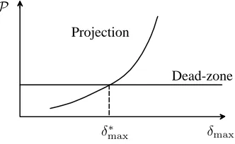
∀dmax≥, ∃δmax∗ ≥δsuch that∀δmax≥δmax∗ ,
P( Σ (X0(γ),Λ,D()),ΞP(δmax) )
>P( Σ (X0(γ),Λ,D()),ΞD0(dmax) ).
(14)
This theorem can be interpreted as stating that if the a-priori knowledge of the parametric uncertainty levelδmax is
suffi-ciently conservative (δmax ≥δmax∗ ), then the dead-zone based
design will out-perform the projection based design.
δmax
δ∗
max
Projection
Dead-zone
[image:3.612.355.521.478.580.2]P
Figure 1: Statement of the main result
5
Proof of Theorem 4.1
Firstly, we show thatP = ∞for the unmodified design (5), (Proposition 5.3). From this we can show that the projection modification design,ΞP(δmax)(10) has the property thatP →
∞asδmax → ∞(Proposition 5.4). Finally we show thatP <
∞for the dead-zone design,ΞD0(dmax)(7) (Propositions 5.5).
details of the proof for brevity. The complete proof can be found in [11].
In the following, we frequently use the coordinate transforma-tion matricesS, S−1defined by
S:=
B(CB)−1, T
, S−1=
CT, NTT
, N=
(bm−1/bm...b0/bm)T;I(m−1).
(15)
whereT ∈Rn×(n−1)is a basis matrix of kerC. Observe that
S, S−1depend continuously onθover∆(δ), and
¯
x(t) := (y(t), z(t)T)T =S−1x(t), (16)
therefore
˙
y(t) ˙
z(t)
=
¯
a1−bmk(t) A¯2
¯
A3 A¯4
y(t)
z(t)
(17)
where¯a1∈R,A¯T2,A¯3∈Rn−1andA¯4∈R(n−1)×(n−1). Note
that¯a1−bmk(t)<0, ∀t > t∗for sufficiently largek∗. It has
been shown that A¯4 is stable [3], i.e. there exists a positive
definite matrixR=RT >0satisfying the Lyapunov equation
RA¯4+ ¯AT4R=−In−1.
We also frequently use the compact notation D(k) := A−
kBC for some k > 0, and D¯ := S−1DS. Note that
¯
D(k∗)TP +PD¯(k∗) ≤ −Q, where the symmetric positive definite matricesP, Qare defined as
P =
1
2 0
0 R
, Q=
1 0
0 12In−1
. (18)
This can be shown by considering the Lyapunov functionV = ¯
xTPx¯and observing that ˙
V = ¯xT D¯(k)TP+PD¯(k) ¯
x
≤ −(bmk(t)−M)y(t)2− 1 2kz(t)k
2
≤x¯TQ¯x, (19)
for allk > k∗, whereM :=|¯a
1|+ kA¯2k+ 2kRk kA¯3k 2
/2,
andk∗:= (M+ 1/2)/b
m.
Lemma 5.1. Consider the systemz˙=f(z)wheref is contin-uous. Thenlimt→∞z(t) =z∗implies thatz∗is an equilibrium point.
Proof. See Lemma 4.3 in [11].
Proposition 5.1. Consider the closed loop system
(Σ(x0, θ, d(·)),Ξ) defined by (2), (5), where C1,C2 hold
andd(t) =for some6= 0. Then
kx(t)k →0 ast→ ∞ ⇐⇒δˆ(t)→ ∞ast→ ∞. (20)
Proof. →) Suppose for contradiction δˆ(t) 6→ ∞. Then
ˆ
δ(t)→δˆ∗<∞, sinceˆδ(t)is monotonic by (5). There-fore (x(t),ˆδ(t)) = (0,δˆ∗) is an equilibrium point of
closed loop (Σ(x0, θ, d(·)),Ξ) by Lemma 5.1. Hence
(0,δˆ∗)must be a solution of the following equations:
x2(t)−an−1x1(t) +bm(−ˆδ(t)x1(t)) = 0,
.. .
−a0x1(t) +b0(−ˆδ(t)x1(t)) = 0, (21)
x1(t)2 = 0.
Butb0 6= 0 since system is minimum phase. We also
have6= 0. Therefore(x(t),δˆ(t)) = (0,δˆ∗)cannot be a solution of (21), hence contradiction.
←) Define the Lyapunov functionV(¯x(t)) = ¯x(t)TP¯x(t),
wherex¯(t), P are defined by (16) and (18) respectively. DenoteB¯ =S−1Band¯b= (P+PT) ¯B. Define
ϕ(t) :=¯x(t)TPD¯(ˆδ(t)−k∗)
+ ¯D(ˆδ(t)−k∗)TPx¯(t). (22)
and note that asˆδ(t)→ ∞we haveϕ(t) → −∞for all
¯
x(t) 6= 0. A routine calculation of the time derivative of
V(¯x(t))implies:
˙
V(¯x(t))≤ −x¯(t)TQx¯(t) + ¯x(t)T¯b+ϕ(t), (23)
≤ −λ(Q)kx¯(t)k2+k¯x(t)k |¯b| ||+ϕ(t).(24) Applying Young’s inequality to (24), we observe thatV(·)
is decreasing if
λ(Q)kx¯(t)k2
2 −ϕ(t)≥ |¯b|2||2
2λ(Q). (25)
Now, we claim the convergence of ¯x(·): if kx¯(t)k 6→ 0 as t → ∞ then either 1. lim inf
t→∞ k¯x(t)k>0 or 2.
lim inf
t→∞ kx¯(t)k= 0: 1. Supposelim inf
t→∞ k¯x(t)k>0. Then there exists 0>
0 s.t. kx¯(t)k > 0 ∀t > 0. Sinceϕ(t)→ −∞as
ˆ
δ(t) → ∞, it follows by (23) that V˙ → −∞ as
t→ ∞, i.e.V → −∞. This contradicts the positive definiteness ofV(·).
2. Iflim inf
t→∞ k¯x(t)k= 0, then there must exists 0>0, and a positive divergent sequence{tk}k≥1such that
˙
V(¯x(tk)) > 0 andk¯x(tk)k > 0. Sinceϕ(tk) →
−∞ask→ ∞, it follows that (25) holds at timetk,
hence contradiction.
Thereforek¯x(t)k → 0as t → ∞; hencex(t) → 0 by (16).
Proposition 5.2. Consider the closed loop system
(Σ(x0, θ, d(·)),Ξ) defined by (2), (5), where C1,C2 hold
andd(t) =for some6= 0. Ifx(t)is uniformly continuous, then ast→ ∞
Proof. Firstly we show thaty(t) → 0ast → ∞. From this we will prove thatδˆ(t) → ∞and finally by Proposition 5.1, we conclude thatkx(t)k →0ast→ ∞. Suppose for contra-dictiony(t)6→0. Then there must exists a positive divergent sequence{tk}k≥1 for whichy(tk) ≥ M for someM > 0.
Sincex(t)is uniformly continuous, it follows thaty(t)is uni-formly continuous, i.e. for=M/2
∃ω >0s.t.∀τ∈[0, ω], ∀t >0, |y(t)−y(t+τ)|< M
2 .
(27) Therefore|y(tk)−y(tk+τ)|< M/2and sincey(tk)≥M, we
have thaty(tk+τ)> M/2i.e.y(t)≥M/2for allt∈[tk, tk+
ω]. With no loss of generality, we may assumetk+1−tk≥ω.
It follows that
ˆ
δ(tk+ω) = Z tk+ω
0
˙ˆ
δ(τ)dτ = Z tk+ω
0
y2(τ)dτ ≥ M
2
4 kω,
(28) soδˆ(tk+ω)→ ∞ask → ∞. It follows by Proposition 5.1
thatkx(t)k →0ast → ∞, thereforey(t)→0by (2), hence contradiction.
Now we have y(t) = x1(t) → 0 and we claimˆδ(t) → ∞.
Suppose for contradictionδˆ(t)6→ ∞. Thenδˆ(t)→ˆδ∗ <∞, sinceˆδ(t)is monotonic by (5). Substitute this into (2), we have
˙
x1(t) = x2(t)−(an−1+ ˆδ∗bm)x1(t) +bm, (29)
.. .
˙
xn(t) = −(a0+ ˆδ∗b0)x1(t) +b0, (30)
where by minimum phase property of system, bi 6= 0, i ∈ [0, m]. Asx1(t)→0, equation (30) implies thatxn(t)→ ∞,
sincex(·)is uniformly continuous. It follows thatxn−1(t)→
∞, and cascading the argument yields tox1(t)→ ∞ast →
∞, hence contradiction. Thereforeδˆ(t)→ ∞. From this and Proposition 5.1, the claim of the proposition follows.
Proposition 5.3. Consider the closed loop system
(Σ(x0, θ, d(·)),Ξ) defined by (2), (5) where C1,C2 hold.
Let Λ ⊂ ∆(δ) be compact. Consider the transient perfor-mance cost functional (12). Then
P( Σ (X0(γ),Λ,D()),Ξ) =∞. (31)
Proof. Let x0 ∈ X0(γ), θ ∈ Λ, and choose d(t) =
6= 0. Denotelim sup t→∞
bylim. Suppose for contradiction
P(Σ(x0, θ, d(·)),Ξ)<∞. Considerx˙(t). There are two cases
either 1.limkx˙(t)k=∞or 2.limkx˙(t)k<∞:
1. Suppose limkx˙(t)k = ∞, i.e.
limkAx(t) +Bu(t) +Bk=∞. Therefore either (a) limkx(t)k = ∞, which implies that kx(·)kL∞ =
∞, hence contradiction, or
(b) limkx(t)k < ∞, therefore lim u(t) = ∞ i.e.
ku(·)kL∞ =∞. Hence contradiction.
2. Supposelimkx˙(t)k <∞i.e. x(·)is uniformly continu-ous. Therefore by Proposition 5.2
kx(t)k →0, δˆ(t)→ ∞ as t→ ∞. (32) Consideringlim ˙u(t), we observe that
lim ˙u(t) =lim
−y(t)3− ˆ
δ(t)CAx(t)−CBˆδ(t)y(t)−i.
(33) Note thatCB 6= 0since the relative degreeρ= 1. Now there are two possible cases, either a)δˆ(t)y(t)6→ (in-cluding the possibility thatlimt→∞ˆδ(t)y(t)does not ex-ist), or b)limt→∞ δˆ(t)y(t) =
(a) Suppose limt→∞δˆ(t)y(t) does not exist or
ˆ
δ(t)y(t) 6→ as t → ∞. It follows by (32) that
ku˙(·)kL∞ =∞; hence contradiction.
(b) Supposelimt→∞δˆ(t)y(t) =. By (32) we have that
∀δˆ∗ >0 ∃T >0 s.t. ∀t > T δˆ(t)>δˆ∗. (34) Now we choose d2(t) := , ∀t ≤ T, d2(t) :=
−, ∀t > T. Note thatd2(t) = d(t)for all t ≤
T. With this choice, by continuity and causality, we have that
lim
t→T+x(t) =x(T), t→limT+
ˆ
δ(t) = ˆδ(T) (35)
wherelimt→T+denotelimt→T ,t>T. It follows that
lim t→T+u˙(t)
−u˙(T) = 2ˆδ(T)CB≥2ˆδ∗b
m.
(36) By choosing a suitableδˆ∗, it follows thatˆδ(T)can be made arbitrarily large and hence the difference (36) is arbitrarily large. Then either u˙(T)is large orlimt→T+u˙(t)is large, thereforeku˙(·)kL∞can be
made arbitrarily large. Hence contradiction.
Therefore at least one component of (12) diverges, hence
P(Σ (X0(γ),Λ,D()),Ξ)≥ P(Σ(x0, θ, d(·)),Ξ) =∞.
(37)
Proposition 5.4. Consider the closed
(Σ(x0, θ, d(·)),ΞP(δmax)) defined by (2), (10) where
C1,C2 hold. Let Λ ⊂ ∆(δ) be compact. Consider the transient performance cost functional (12). Then
P(Σ (X0(γ),Λ,D()),ΞP(δmax))→ ∞ as δmax→ ∞.
(38)
Proof. It is convenient to define
P[0,T](Σ(x0, θ, d(·)),Ξ)
=kx(·)kL∞
[0,T]+ku(·)kL∞
[0,T]+ku˙(·)kL∞
[0,T]
Now let M > 0. By Proposition 5.3 there existsx0 ∈ X0,
d(·)∈ D(),θ∈Λso that
P[0,∞)(Σ(x0, θ, d(·)),Ξ)≥2M. (40)
It follows that ∃T > 0 s.t. P[0,T](Σ(x0, θ, d(·)),Ξ) ≥ M.
Sinceδmaxdiverges, by choosingδmax = 2ˆδ(T), we have that
δmax > δˆ(T), i.e. the unmodified and the projection designs
are identical on[0, T], therefore
P(Σ (X0(γ),Λ,D()),ΞP(δmax))
≥ P[0,T](Σ(x0, θ, d(·)),ΞP(δmax))≥M.
(41)
Since this holds for allM >0, this completes the proof. Proposition 5.5. Consider the closed loop
(Σ(x0, θ, d(·)),ΞD0(dmax)) defined by (2), (7) where
C1,C2 hold. Let Λ ⊂ ∆(δ) be compact. Consider the transient performance cost functional (12). Then
P(Σ (X0(γ),Λ,D()),ΞD0(d
max))<∞, ∀dmax> . (42)
Proof. Let x0 ∈ X0(γ), θ ∈ Λandd ∈ D(). A direct
ap-plication of Property P2 of Theorem 3.1 guarantees the uni-formly boundedness ofx(·),δˆ(·), u(·)as a continuous function ofV∗(x
0, θ, dmax). It follows that
˙
u(t) =−D0
Ω0|y(t)|y(t)
2
−δˆ(t)CA−δˆ(t)BCx(t) +Bd(t), (43)
is uniformly bounded in terms of a continuous function of
V∗(x
0, θ, dmax). Therefore
P(Σ(x0, θ, d(·)),ΞD0(dmax))≤M(V∗(x0, θ, dmax)), (44)
for some continuous M(V∗(x
0, θ, dmax) < ∞. Taking the
supremum over system parametersx0, θ, dimplies that for all
dmax≥,
P(Σ (X0(γ),Λ,D())ΞD0(d
max))
≤ sup x0∈X0(γ)
sup θ∈Λ
sup d∈D()
M(V∗(x0, θ, dmax))<∞. (45)
Proof of Theorem 4.1.
This is a simple consequence of Proposition 5.4 and Proposi-tion 5.5.
6
Conclusion
In this paper we have established a rigourous result which demonstrate a situation in which we can compare the transient performance of projection and dead-zone based controllers of non identifier based adaptive designs. There are a number of directions in which the result can be generalised, for example: generalisation of the result for higher relative degrees and es-tablishing whether the same results can be given for the alter-native costs, for example, P =kx(·)kL∞+ku(·)kL∞.
Sim-ilarly we have developed results to demonstrate the contrary relationship between the controllers, ie. the results which show when the projection controllers outperform the dead-zone con-trollers, [11].
References
[1] C. I. Byrnes and J. C. Willems. Adaptive stabilization of multivariable linear systems. In Proc. 23rd IEEE Confer-ence on Decision and Control, pages 1574–1577, 1984.
[2] B. Egardt. Stability of adaptive controllers. Lecture notes in Control and Information Sciences, Springer–Verlag, New York, 1979.
[3] A. Ilchmann. Non–Identifier–Based High–Gain Adaptive Control. Lecture notes in Control and Information Sci-ences, Springer–Verlag, London, 1993.
[4] G. Kreisselmeier and K. S. Narendra. Stable model refer-ence adaptive control in the presrefer-ence of bounded distur-bances. IEEE Trans. on Automatic Control, 27(6):1169– 1175, 1982.
[5] M. Krsti´c, I. Kanellakopoulos, and P. Kokotovi´c. Nonlin-ear and Adaptive Control Design. John Wiley & Sons, New York, 1995.
[6] B. M˚artensson. The order of any stabilizing regulator is sufficient a priori information for adaptive stabilization. Systems and Control Letters, 6:87–91, 1985.
[7] A. S. Morse. An Adaptive Control for Globally Stabiliz-ing Linear Systems with Unknown High–frequency Gain. Springer–Verlag, Berlin, 1984.
[8] K. S. Narendra and A. M. Annaswamy. Stable Adaptive Systems. Prentice–Hall, 1989.
[9] R. D. Nussbaum. Some remarks on a conjecture in pa-rameter adaptive control. Systems and Control Letters, 3:243–246, 1983.
[10] B. B. Peterson and K. S. Narendra. Bounded error adaptive control. IEEE Trans. on Automatic Control, 27(6):1161–1168, 1982.