Abstract—In this paper, an integrated inventory model with preventive maintenance based on rapid was built Besides the common topics such as imperfect production process, preventive maintenance, repair, and rework for researches of production and inventory model in recent years, this study featured with the assumption that “How to check a production system fails or not?” which was seldom mentioned in the past. The minimal total cost could be figured out with an optimal inventory cycle and times of deliveries which derived from the algorithm in this paper. Finally, a numerical example and sensitivity analyses were demonstrated in the end of this paper.
Index Terms—Integrated inventory model, Preventive maintenance, Rapid inspection, Optimal
I. INTRODUCTION
S the beginning section, we would explain the structure of this paper: literature review would be shown in section II. An integrated preventive maintenance inventory model would illustrate in section III, the preventive maintenance (PM) program involved rapid inspection, perfect repair, and rework. The goal of this paper is to determine the optimal inventory cycle from the integrated inventory model and the related times of delivery, and figure out the minimal total cost—including the setup, holding, PM, perfect repair, rapid inspection, and rework cost. Section IV would provide numerical examples and sensitivity analysis. Finally, Section V concluded this paper.
II.LITERATUREREVIEW
Inventory management plays an important role in today’s business environment. According to Blevins et al., inventory is listed as an asset on a firm's balance sheet and consists of the stocks or items needed to maintain production, support activities such as maintenance and repair, and provide customer relations. Inventory typically is categorized based on its flow through the production cycle, using such designations as raw materials, work in process, and finished goods. maintenance, repair, and operating supplies also are Min-Der Ko is with the Department of Transportation Science, National Taiwan Ocean University, Keelung 20224 Taiwan (phone: +886-2-2462-2192 #7029; e-mail: [email protected]).
Chien-Chi Wang was with the Department of Transportation Science, National Taiwan Ocean University, Keelung 20224 Taiwan (phone: +886-2-2462-2192 #7011; e-mail: [email protected]).
Ming-Feng Yang is with the Department of Transportation Science, National Taiwan Ocean University, Keelung 20224 Taiwan (phone: +886-2-2462-2192 #7031; e-mail: [email protected]).
stocked to support the functionality of the firm [1]. A well-designed inventory and production policies for manufacturers are key factors to meet today’s highly competitive and uncertainty global market. Product reliability and uniformity must be incorporated into the equipment’s operating conditions. Through maintenance, a highly reliable system can be achieved. Hence, production policy is increasingly dependent on the maintenance programming [2]. The well-known economic order quantity (EOQ) model was proposed by Harris [3]. The economic production quantity (EPQ) model can be deemed as an extension of the EOQ model. By Employing this methodology can lead to a high-quality customer service. However, this model was restricted by many assumptions. The traditional EPQ model assumed defect-free production system output, however, random failure of production equipment is inevitable. Lot of results have been reported in the researches in which these assumptions could be relaxed. After periods of production runtime, the process would shift to an “out-of-control” state, and defective items would be produced until repair is performed to return the process to an “in-control” state. Such this production process is known as “imperfect production process” [4-7].
One way to keep production system stable and avoid manufacture process being out of control is Preventive Maintenance (PM). Barlow and Hunter [8] developed a model of preventive maintenance to keep the efficacy of the production system by regular maintenance. PM contains all operations intended to avoid the major failure or a higher cost at a later stage by maintaining the components of the machines used to manufacture the products at a safe and operational condition [9]. One of a major goal of production improvement is optimization for effectiveness of equipment. But PM is not always perfect. In practice, imperfect PM may result from many reasons and it may be even much more frequent than perfect PM. In several studies have ever considered the assumption of imperfect PM [10-12]. Liao developed an EPQ model of randomly failing process with minimal repair, backorder and preventive maintenance. This study found that enhancing maintenance ability reduced production related cost. The product system can be produced more efficiently using a PM program [13]. Then he modified this model and raised another integrated EPQ model which incorporated FRW, production, and maintenance programs. This model considered the effect of actions such as repair, rework, and PM on a deteriorating production system. The results of his paper demonstrated that such a policy is more flexible and widely applicable than previous policies [14].
Optimal Integrated Inventory Model with
Preventive Maintenance Program based on
Rapid Inspection
Min-Der Ko, Chien-Chi Wang, and Ming-Feng Yang
A
IAENG International Journal of Applied Mathematics, 49:4, IJAM_49_4_02
To keep competitive in today’s rapid-changing business environment, interaction and relationship between members in supply chain should be much closer. Supplier and buyer coordinate closely as the stable long-term relationship would be helpful for problem solving and gain more benefits together [15]. Such an integrated inventory model may be a solution for supply chain collaboration. Goyal illustrated the first integrated inventory model; he deduced that the optimal order time interval and production cycle time can be obtained by assuming that the supplier’s production cycle time is an integer multiple of the customer’s order time interval [16]. Lot of researches also noted that the integrated model with stronger cooperation between the buyer and the supplier would bring better performance [17-20]. Yang et al. [21] built an integrated inventory model with decreasing probability of imperfect maintenance, this model taken the assumptions of imperfect production process and imperfect preventive maintenance into consideration to vender-buyer. Base on earlier studies, Yang and Lin [22] extended and proposed an integrated inventory model with the consideration of incorporating production programs and two types of preventive maintenances to an imperfect process involving a deteriorating production system. They derived an optimal number of shipments and lower cost then found that the demand and production ratio influenced the holding cost and purchase cost and has the most obvious impact on the integrated model.
We have reviewed lot of relevant researches with the topics of integrated inventory model, imperfect production process, preventive maintenance program. Generally, the studies about preventive maintenance program were all based on the assumption of imperfect production process. But most of these papers did not describe that “How to confirm that whether the production system fails or not?”. So, that right the topic which is worthy to be extended. This paper was mainly extended from the study of Fang et al. [2] in International MultiConference of Engineers and Computer Scientists 2019. Apart from the topics we mentioned above, this study added more detailed setting on rapid inspection which was a different inspection method from the conference paper.
III. MODELBUILDING
The relevant assumptions of this study are defined and extended from the study of Fang et al. [2] in International MultiConference of Engineers and Computer Scientists 2019. At the beginning of this section, we would describe the difference between “inspection” of Fang’s model and “rapid inspection” in this study.
In Fang’s model, inspection activity was only conducted to defective item after production runtime period when system fail in the same inventory cycle. This study defined rapid inspection as an examining method for quality control and health of production system. It would classify every item into standard product or defective product while items completed its production process in production runtime no matter system fail or not. The definition of notation in the integrated inventory model were arranged in section B of Appendix. The assumptions to build the integrated inventory model in detail would be shown as below:
A. Assumptions
1. There is only one kind of product in the production system with single vender and single buyer.
2. Production rate, demand rate, setup cost, ordering cost, holding cost, PM cost, inspection cost, perfect repair cost, and rework cost are assumed known.
3. Lead time and delivery time are assumed as 0.
4. The term T denotes a whole inventory cycle and it could be divided into two periods:
a) (𝑑/𝑝)𝑇 represents the inventory building period (production running period).
b) (1 − 𝑑/𝑝)𝑇 represents the inventory depletion period (PM or perfect repair period).
5. Backorder is not permitted.
6. Once the vendor receives an order, the production operation will start until the quantity reach to QL. 7. The items would be delivered from vendor to buyer by
each Q unit, and there are L lots of items would be delivered in an inventory cycle.
8. The operation of original system begins at time 0, the production process begins in an “in-control” state, setup cost occurs at the start of each inventory cycle. 9. Rapid inspections are conducted to every item after it
complete the production process and inspection cost is incurred.
10. There may inevitably be few items which produced under “in-control” state defective but all of them are assumed negligible.
11. PM would be performed following the production running period at cumulative production runtime
𝑗(1 − 𝑑/𝑝)𝑇 for (j = 1, 2, …) by one of the following two results:
a) Perfect PM obtains an as-good-as-new units, with probability 𝜃𝑗= 1 − 𝑞𝑗.
b) Imperfect PM results in the units with the same failure rate as last PM, with probability 𝑞𝑗=
𝑃̅𝑗
𝑃̅𝑗−1
for (0 ≤ 𝑞𝑗≤ 1).
12. If system fail, it will shift into the “out-of-control” state, the items produced under this state are all assumed defective and there is no PM conducted in this inventory cycle.
13. Perfect repair would be performed to the failed system and defective items would be reworked after this production running period in the same cycle.
14. After perfect repair or perfect PM, the system would be refreshed as good as new. The system returns to time 0. 15. The time of PM or perfect repair are not a constant, but
they must be less than or equals to (1 − 𝑑/𝑝)𝑇. The general model of integrated inventory model would include function of vendor’s total expected cost (TECv), buyer’s total expected cost (TECb), and their combination: united total expected cost (UTEC). The assumption of the above function in mathematics would be shown as below:
IAENG International Journal of Applied Mathematics, 49:4, IJAM_49_4_02
B. Vendor’s Total Expected Cost
If the jth instance of the PM is performed, then it is either
imperfect or perfect. Let W denote the cumulative production runtime to a failure of a new system. For the present policy
𝑈𝑗= {
𝑊 − (𝑗 − 1) (𝑑
𝑝) 𝑇, 𝑖𝑓 (𝑗 − 1) ( 𝑑
𝑝) 𝑇 < 𝑊 < 𝑗 ( 𝑑 𝑝) 𝑇
(𝑑
𝑝) 𝑇, 𝑖𝑓 𝑊 ≥ 𝑗 ( 𝑑 𝑝) 𝑇
for j =1, 2, …
(1) Where Uj represents the in-control production runtime during the jth inventory cycle after (j–1) imperfect PMs. As
mentioned earlier, we use the concept of an imperfect PM. Note that the probability after (j–1) imperfect PMs is given by for ∑ 𝑃̅𝑗−1𝑃̅
𝑗−1 ∞
𝑗=1 for (j = 1, 2, …). Thus, expected time of an
in-control production run is:
∑ 𝐸[𝑈𝑗] ∞
𝑗=1
= ∑ 𝑃̅𝑗−1 ∑∞𝑗=1𝑃̅𝑗−1 ∞
𝑗=1
×
{
∫ [t − (𝑗 − 1) (𝑑
𝑝) 𝑇] 𝑓(𝑡)𝑑𝑡
𝑗(𝑑 𝑝)𝑇
(𝑗−1)(𝑑𝑝)𝑇
+ (𝑑 𝑝) 𝑇𝐹̅(𝑗(
𝑑 𝑝)𝑇)
}
= ∑(𝑃̅𝑗−1− 𝑃̅𝑗) ∑∞𝑗=1𝑃̅𝑗−1 ∞
𝑗=1
∫ 𝐹̅(𝑡)𝑑𝑡
𝑗(𝑑𝑝)𝑇
0 (2)
Let Rj denote the total PM costs, restoration costs (rework cost and perfect repair cost) during the jth inventory cycle, R
j could be presented as:
∑ 𝐸[𝑅𝑗] ∞
𝑗=1
= ∑ 𝐸 [𝑅𝑗, 𝑊 ≥ 𝑗 (
𝑑 𝑝) 𝑇]
∞
𝑗=1
+ ∑ 𝐸 [𝑅𝑗, (𝑗 − 1) (
𝑑
𝑝) 𝑇 < 𝑊 < 𝑗 ( 𝑑 𝑝) 𝑇]
∞
𝑗=1 (3)
According to the 11th point of the assumptions, PM would
be performed after the in-control production running period. That is, 𝑊 ≥ 𝑗 (𝑑
𝑝) 𝑇 for (j = 1, 2, …) following (j–1) imperfect PMs. So, the expected PM cost in an inventory cycle would be:
1
𝑇∑ 𝐸 [𝑅𝑗, 𝑊 ≥ 𝑗 ( 𝑑 𝑝) 𝑇] =
𝐾𝑝𝑚
𝑇 ∑ 𝑃̅𝑗−1
∑∞𝑗=1𝑃̅𝑗−1
𝐹̅(𝑗 (𝑑 𝑝) 𝑇)
∞
𝑗=1 ∞
𝑗=1 (4)
If the system falls into the “out-of-control” state, restoration activities will be conducted after this production running period. Perfect repair action can restore the production system to such as a brand-new state. The expected number of defective items would be:
𝑝 × (expected out-of-control production runtime)
= 𝑝
[ (𝑑
𝑝) 𝑇 − ∑
(𝑃̅𝑗−1− 𝑃̅𝑗)
∑∞𝑗=1𝑃̅𝑗−1 ∞
𝑗=1
∫ 𝐹̅(𝑡)𝑑𝑡
𝑗(𝑑 𝑝)𝑇
0
] (5)
According to the 13th point of the assumptions, the
expected restoration cost in an inventory cycle would be:
1
𝑇∑ 𝐸 [𝑅𝑗, (𝑗 − 1) ( 𝑑
𝑝) 𝑇 < 𝑊 < 𝑗 ( 𝑑 𝑝) 𝑇]
∞
𝑗=1
=1
𝑇(expected perfect repair cost + expected rework cost)
=𝐾𝑟 𝑇∑
𝑃̅𝑗−1
∑∞𝑗=1𝑃̅𝑗−1 ∞
𝑗=1
𝐹((𝑑 𝑝) 𝑇) +
𝐾𝑟𝑤𝑝
𝑇 {( 𝑑
𝑝) 𝑇 − ∑ 𝐸[𝑈𝑗]
∞
𝑗=1
} (6) Fig.1 displayed the idea of production system with PM and perfect repair strategy; and the accumulated inventory for buyer was illustrated in Fig.2. Once vendor receives an order, vendor will start to produce immediately until the quantity reach to QL. Products will be delivered from vendor to buyer by each Q unit, and there are L lots of products will be delivered in an inventory cycle. The average inventory of vendor could be evaluated as function (7):
Fig.1 Production system with PM and perfect repair strategy
Fig.2 Accumulated inventory for buyer
The routine cost of vendor in this model would contain setup cost, holding cost, and rapid inspection cost as following list:
Quantity
W - ( j-1)(d/p)T j(d/p)T Time
(d/p)T (1- d/p)T
production running period inventory depletion period
The jth Inventory Cycle ( for j = 1, 2, 3,…)
: Quantity of defective item.
: Time point that production system shifts into "out of control" state.
Quantity
LQ/p
QL
QL / d Time
Accumulated Inventory for Vendor
Accumulated Inventory for Buyer
IAENG International Journal of Applied Mathematics, 49:4, IJAM_49_4_02
1) Setup cost: 𝐾𝑠 𝑇
2) Holding cost(v): 𝐾ℎ𝐾𝑣[𝐼𝑣] 3) Inspection cost: 𝐾𝑖𝑑
According to the assumptions and idea of Fig.2, the accumulated inventory produced by vendor could be present as below:
𝐼𝑣=
{[𝑄𝐿 (𝑄
𝑝+ (𝐿 − 1) 𝑄 𝑑) −
𝑄2𝐿2
2𝑝 ] − [ 𝑄2
𝑑(1 + 2 + ⋯ + (𝐿 − 1))]}
(𝑄𝐿𝑑)
=𝑄𝐿 2 [(1 −
𝑑 𝑝) − 1 +
2𝑑
𝑝] (7)
Let TECv be the total expected cost of vendor, according to the above descriptions and notations, TECv could be present as below:
TECv = Routine cost + PM cost + Restoration cost
C.Buyer’s Total Expected Cost
Let TECb be total expected cost of buyer. It includes ordering cost and holding cost.Then TECb could be present as below:
1) Ordering cost: L𝐾𝑜 2) Holding cost(b): 𝐾ℎ𝐾𝑝
𝑄 2
According to Fig.2, 𝑇 = 𝑄𝐿/𝑑,so holding cost of vendor and buyer could be rewritten as:
𝐾ℎ𝐾𝑝
𝑄
2+ 𝐾ℎ𝐾𝑣[𝐼𝑣] = 𝑇𝑑
2𝐿(𝐾ℎ𝐾𝑝+ 𝐾ℎ𝐾𝑣{𝐿 [(1 − 𝑑 𝑝) − 1 +
2𝑑
𝑝]}) (8)
D.United Total Expected Cost
Let’s unite TECvand TECb and let {T, L} as the decision variables in this model, then we could get UTEC(T, L), the
function of united total expected cost in an inventory cycle as below:
𝑈𝑇𝐸𝐶(𝑇,𝐿) =𝑇𝑑
2𝐿(𝐾ℎ𝐾𝑝+ 𝐾ℎ𝐾𝑣{𝐿 [(1 − 𝑑 𝑝) − 1 +
2𝑑 𝑝]})
+1 𝑇
{
𝐾𝑠+ 𝐿𝐾𝑜+ 𝐾𝑖𝑇𝑑 + 𝐾𝑝𝑚∑
𝑃̅𝑗−1
∑∞𝑗=1𝑃̅𝑗−1
𝐹̅(𝑗 (𝑑 𝑝) 𝑇)
∞
𝑗=1
+𝐾𝑟∑
𝑃̅𝑗−1
∑∞𝑗=1𝑃̅𝑗−1 ∞
𝑗=1
𝐹((𝑑 𝑝) 𝑇)
+𝐾𝑟𝑤𝑝
[ (𝑑
𝑝) 𝑇 − ∑
(𝑃̅𝑗−1− 𝑃̅𝑗)
∑∞𝑗=1𝑃̅𝑗−1 ∞
𝑗=1
∫ 𝐹̅(𝑡)𝑑𝑡
𝑗(𝑑𝑝)𝑇
0
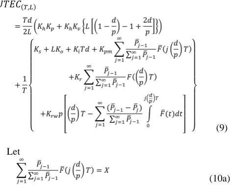
] } (9) Let
∑ 𝑃̅𝑗−1 ∑∞𝑗=1𝑃̅𝑗−1
𝐹̅(𝑗 (𝑑 𝑝) 𝑇)
∞
𝑗=1
= 𝑋
(10a)
∑ 𝑃̅𝑗−1 ∑∞𝑗=1𝑃̅𝑗−1 ∞
𝑗=1
𝐹(𝑗 (𝑑
𝑝) 𝑇) = 𝑌 (10b)
∑(𝑃̅𝑗−1− 𝑃̅𝑗) ∑∞𝑗=1𝑃̅𝑗−1 ∞
𝑗=1
∫ 𝐹̅(𝑡)𝑑𝑡
𝑗(𝑑𝑝)𝑇
0
= 𝑍
(10c) Then UTEC(T, L) could be show as bellows:
𝑈𝑇𝐸𝐶(𝑇,𝐿)
=𝑇𝑑
2𝐿(𝐾ℎ𝐾𝑝+ 𝐾ℎ𝐾𝑣{𝐿 [(1 − 𝑑 𝑝) − 1 +
2𝑑 𝑝]})
+1 𝑇{
𝐾𝑠+ 𝐿𝐾𝑜+ 𝐾𝑖𝑇𝑑
+𝐾𝑝𝑚𝑋 + 𝐾𝑟𝑌 + 𝐾𝑟𝑤𝑝 [(
𝑑 𝑝) 𝑇 − 𝑍]
}
(11)
Theorem 1:
Let’s take first-order partial derivative of UTEC(T ,L) by T
with the given L to get equation (12) and make it equal to zero, we could get the optimal T* where the mark “ * ” denoted the optimal value.
𝜕𝑈𝑇𝐸𝐶(𝑇,𝐿)
𝜕𝑇
= 𝑑
2𝐿(𝐾ℎ𝐾𝑝+ 𝐾ℎ𝐾𝑣{𝐿 [(1 − 𝑑 𝑝) − 1 +
2𝑑 𝑝]})
+1 𝑇2{
−𝐾𝑠− 𝐿𝐾𝑜+ 𝐾𝑝𝑚(−𝑋 + 𝑇𝑋′)
+𝐾𝑟𝑤𝑝(−𝑌 + 𝑇𝑌′) + 𝐾𝑟𝑤𝑝(𝑍 − 𝑇𝑍′)
}
(12) Then we toke second-order partial derivative of UTEC(T, L)
by T with the given L to get equation (13), if the result of equation (13) > 0, then there existed a finite and unique optimal solution {T*, L} to minimize UTEC
(T, L).
𝜕2𝑈𝑇𝐸𝐶 (𝑇,𝐿)
𝜕𝑇2 =
1 𝑇3{
𝐾𝑠+ 𝐿𝐾𝑜+ 𝐾𝑝𝑚(𝑋 − 2𝑇𝑋′+ 𝑇2𝑋′′)
+𝐾𝑟(𝑌 − 2𝑇𝑌′+ 𝑇2𝑌′′) + 𝐾𝑟𝑤𝑝(−𝑍 + 2𝑇𝑍′− 𝑇2𝑍′′)
} (13)
Proof : See Appendix
The process to gain the minimal UTEC(T*) and related
optimal T* had been shown on the above. In addition, we still wanted to figure out the optimal number of deliveries lots by the integrated inventory model. So, we built an algorithm to figure out the minimal UTEC(T, L) and related {T*, L*}. The
procedure to determine the minimal UTEC(T, L) and related
{T*, L*} in the integrated inventory model were showed on Algorithm 1 in Appendix:
IV. NUMERICALEXAMPLE
To demonstrate the integrated model, we applied the PM policy of Nakagawa who applied an imperfect PM model in which PM yields a system as bad as old with probability p
and as good as new with probability 𝑝̅ = 1 − 𝑝 [23]. Based on this PM policy, we presented three cases of sensitivity analyses in this policy. We set the case of probability imperfect PM q as Case 1; case of ratio of demand rate to production rate d/p as Case 2; and case of multiple of d and p
as Case 3. The general parameters setting was shown in table
IAENG International Journal of Applied Mathematics, 49:4, IJAM_49_4_02
[image:4.595.50.286.581.773.2]I. The result of Case 1 showed on Table II and Fig.3. The result of Case 2 showed on Table III, Table IV, Fig.4, and Fig.5, where p = 1,000 and fixed, L = 9 and fixed. The result of Case 3 showed on Table V and Fig.6, where d = 700, p = 1,000 for multiple = 1, L = 9 and fixed.
TABLEI
GENERAL SETTING OF SENSITIVITY ANALYSES
Parameters Setting
d 700 units per year
p 1,000 units per year
Ko $ 12 each order Kh $ 3 per unit Kv $ 20 per unit Kp $ 25 per unit Ki $ 0.1 per unit Krw $ 2 per unit
Ks $ 200 for each production run Kpm $ 300 per time of PM Kr $ 400 per time of perfect repair
𝐹(𝑡) Following a Gamma cumulative distribution
with α = 2, β = 1
TABLEII
SENSITIVITYANALYSISINCASE1
q
L
T* UTEC(T*, L)
0.01 0.25 0.4 0.01 0.25 0.4
1 0.1117 0.1115 0.1113 9,239 9,256 9,278 2 0.1370 0.1367 0.1363 7,722 7,744 7,772 3 0.1509 0.1505 0.1500 7,178 7,202 7,235 4 0.1602 0.1597 0.1591 6,916 6,942 6,977 5 0.1671 0.1666 0.1660 6,775 6,803 6,840 6 0.1727 0.1721 0.1715 6,697 6,726 6,765 7 0.1774 0.1768 0.1761 6,656 6,687 6,727 8 0.1815 0.1809 0.1802 6,639 6,671 6,712 9 0.1852 0.1846 0.1838 6,638 6,670 6,713 10 0.1886 0.1879 0.1871 6,648 6,681 6,725 11 0.1917 0.1910 0.1902 6,666 6,700 6,744 12 0.1947 0.1939 0.1931 6,690 6,725 6,770
TABLEIII
SENSITIVITY ANALYSIS IN CASE 2, RESULT OF T*
d 500 600 700 800 900
d/p 50% 60% 70% 80% 90%
q = 0.01 0.2512 0.2132 0.1852 0.1638 0.1468
q = 0.25 0.2504 0.2125 0.1846 0.1632 0.1462
q = 0.4 0.2494 0.2116 0.1838 0.1625 0.1456
TABLE IV
SENSITIVITY ANALYSIS IN CASE 2, RESULT OF UTEC(T*, L)
d 500 600 700 800 900
d/p 50% 60% 70% 80% 90%
q = 0.01 4,893 5,766 6,638 7,509 8,379
q = 0.25 4,915 5,794 6,671 7,547 8,422
q = 0.4 4,945 5,830 6,713 7,596 8,478
TABLEV
SENSITIVITY ANALYSIS IN CASE 3
multiple of d & p d/p = 0.6 d/p = 0.7 d/p = 08
0.25 0.4218 0.3664 0.3239
0.50 0.2995 0.2602 0.2300
0.75 0.2450 0.2129 0.1882
1 0.2125 0.1846 0.1632
2 0.1506 0.1308 0.1156
5 0.0954 0.0829 0.0733
10 0.0675 0.0586 0.0519
Fig.3 Sensitivity analysis in case 1
Fig.4 Sensitivity analysis in case 2, result of T*
Fig.5 Sensitivity analysis in case 2, result of UTEC(T*, L)
Fig.6 Sensitivity analysis in case 3 0.10 0.11 0.12 0.13 0.14 0.15 0.16 0.17 0.18 0.19 0.20
6,500 7,000 7,500 8,000 8,500 9,000 9,500
1 2 3 4 5 6 7 8 9 10 11 12
T*
U
T
EC
(T
*,
L
)
L
q = 0.01 q = 0.25 q = 0.4 q = 0.01 q = 0.25 q = 0.4
q= 0.4 The bottom line
q= 0.25 The middle line
0.14 0.16 0.18 0.20 0.22 0.24 0.26
50% 60% 70% 80% 90%
T*
d/p
q = 0.01 q = 0.25 q = 0.4
4,400 4,900 5,400 5,900 6,400 6,900 7,400 7,900 8,400 8,900
50% 60% 70% 80% 90%
U
T
EC
(T
*,
L
)
d/p
q = 0.01 q = 0.25 q = 0.4
0.00 0.05 0.10 0.15 0.20 0.25 0.30 0.35 0.40 0.45
0.25 0.5 0.75 1 2 5 10
T*
multiple of d and p
d/p = 0.6 d/p = 0.7 d/p = 0.8
q = 0.01 The top line
q = 0.25 The middle line
q = 0.4 The bottom line
q = 0.01 The top line
IAENG International Journal of Applied Mathematics, 49:4, IJAM_49_4_02
1. For result of Case 1, T* and deviation of T* between
different level of q rise by increasing of L. This result showed that more times of delivery would make longer of inventory cycle time.
2. By applied Algorithm 1 with the given parameter setting in Case 1, we could observe that when q = 0.01 and 0.25, the optimal {T*, L*} which bring the minimal UTEC occurs at L = 9. But when q rises to 0.4, optimal {T*, L*} which bring the minimal UTEC
occurs at L = 10. This mean the L* is not always fixed,
it may vary with different parameter input.
3. For result of Case 2, T* goes down by increasing of d/p, whereas UTEC(T*, L*) is opposite. This result
show that a shorter inventory cycle must be supported by a higher level of inventory cost. 4. In Case 3, we only showed the outcome of T* caused
under a same level of d/p, UTEC must rise by growth of both production rate and demand rate.
5. For result of Case 3, the T* goes shorter by growth of
multiples of production rate and demand rate, and the more multiples grown, the much slightly the T*
vary. By contrast, the more multiple shrink, the much obviously the T* vary.
V.CONCLUSIONS
There were few studies about the topic of imperfect production process considered about the method that how to determine a production system breaks down or not? So, this study built an integrated inventory model with preventive maintenance based on rapid. The assumption of this study was more detailed than the research of Fang et al. [2]. The result of this paper showed that producer should try to keep the production system well and enhance the reliability of products to reduce restoration cost. Furthermore, we also found that multiple times of deliveries would must better than just single time of delivery in an inventory cycle.
To make the proposed integrated inventory model much fit to the reality, such the restriction of unallowable backorder, variance of lead time, change of time value, quantity discount, and allowance of delay of payments could may be released. And to understand the performance of different inspection method, more inspection methods of product could be considered which may bring a higher level of reliability of product.
APPENDIX
A. Proof of Theorem 1
Let H be the Hessian matrix of UTEC(T,L), then UTEC(T,L)
would be concave if equation (13) > 0.
𝐻 =
[ 𝜕2𝑈𝑇𝐸𝐶
(𝑇,𝐿)
𝜕𝑇2
𝜕𝑈𝑇𝐸𝐶(𝑇,𝐿)
𝜕𝑇𝜕𝐿 𝜕𝑈𝑇𝐸𝐶(𝑇,𝐿)
𝜕𝐿𝜕𝑇
𝜕2𝑈𝑇𝐸𝐶 (𝑇,𝐿)
𝜕𝐿2 ]
=𝜕
2𝑈𝑇𝐸𝐶 (𝑇,𝐿)
𝜕𝑇2 ×
𝜕2𝑈𝑇𝐸𝐶 (𝑇,𝐿)
𝜕𝐿2 −
𝜕𝑈𝑇𝐸𝐶(𝑇,𝐿)
𝜕𝑇𝜕𝐿 ×
𝜕𝑈𝑇𝐸𝐶(𝑇,𝐿)
𝜕𝐿𝜕𝑇 (A1)
According to equation (11), (12), and (13): 𝜕2𝑈𝑇𝐸𝐶
(𝑇,𝐿)
𝜕𝑇2 = equation (13) (A2)
𝜕2𝑈𝑇𝐸𝐶 (𝑇,𝐿)
𝜕𝐿2 =
𝑇𝑑𝐾ℎ𝐾𝑝
𝐿3 (A3)
𝜕𝑈𝑇𝐸𝐶(𝑇,𝐿)
𝜕𝑇𝜕𝐿 =
𝜕𝑈𝑇𝐸𝐶(𝑇,𝐿)
𝜕𝐿𝜕𝑇 = −𝑑𝐾ℎ𝐾𝑝
2𝐿2 +
𝐾𝑜
𝑇2 (A4)
Let apply equation (A1), (A2), (A3), and (A4), we could obtain H as equation (A5):
𝐻 = (𝑑𝐾ℎ𝐾𝑝 𝑇2𝐿3) [
𝐾𝑠+ 𝐾𝑝𝑚(𝑋 − 2𝑇𝑋′+ 𝑇2𝑋′′)
+𝐾𝑜+ 𝐾𝑟(𝑌 − 2𝑇𝑌′+ 𝑇2𝑌′′)
+𝑝𝐾𝑟𝑤(−𝑍 + 2𝑇𝑍′− 𝑇2𝑍′′)
]
(A5) If both H and equation (13) > 0, then there existed a finite and unique optimal solution {T*, L} to minimize UTEC
(T, L).
B.Notation
Notation Definition
T Time of an inventory cycle, 𝑇 = 𝑄𝐿/𝑑
W Cumulative production runtime from “in-control” state to “out-of-control” state in a brand-new well system
p Production rate in units per year
d Demand rate in units per year; 𝑝 > 𝑑
Q Order quantity of each delivery
L Times of deliveries in an inventory cycle
Kh Inventory cost rate in unit per year Ks Vendor’s setup cost for each production run Kv Vendor’s production cost per unit, where Kp > Kv Ko Purchaser’s ordering cost for each order Kp Purchaser’s purchase cost per unit Kpm Cost of each PM, where Kr > Kpm Kr Perfect repair cost for each failure Ki Rapid inspection cost per unit
Krw Rework cost of per unit, where Kh > Krw > Ki
𝑃̅𝑗 Probability that the first j PMs are imperfect PMs; 𝑃̅0= 1
𝑞𝑗 Probability that the jth PM is an imperfect PM; 𝑞𝑗= 𝑃̅𝑗/𝑃̅𝑗−1
𝜃𝑗 Probability that the jth PM is a perfect PM; 𝜃𝑗= 1 − 𝑞𝑗
𝑝𝑗 Probability that PM is perfect following the (𝑗 − 1)
imperfect PM; 𝑝𝑗= 𝑃̅𝑗−1𝜃𝑗= 𝑃̅𝑗−1− 𝑃̅𝑗
𝐹(𝑡) Failure distribution function of W
𝑓(𝑡) Failure density function associated with 𝐹(𝑡)
𝐹̅(𝑡) Survival function associated with 𝐹(𝑡)
C.Algorithm 1
Algorithm 1. Determining process of {T*, L*
} and 𝑈𝑇𝐸𝐶∗ Results: {T*, L*
}, 𝑈𝑇𝐸𝐶∗
Step1. Make equation (12) equal to 0 to determine T(L)
Step2. Compute equation (13) with {T(L), L} If The outcome of Step2. > 0
Step3. Compute equation (11) with {T(L), L}
Step4. Repeat Step1. to Step3. with (L + 1)
If 𝑈𝑇𝐸𝐶{𝑇(𝐿),𝐿}< 𝑈𝑇𝐸𝐶(𝑇(𝐿+1),𝐿+1)
Step5. Let {T*, L*}={T(L), L},
and 𝑈𝑇𝐸𝐶∗= 𝑈𝑇𝐸𝐶
{𝑇(𝐿),𝐿} Else Restart from Step1.
Else Abandon the result of current data set, reset data and restart from Step1.
IAENG International Journal of Applied Mathematics, 49:4, IJAM_49_4_02
REFERENCES
[1] P. Blevins et al., C. Daniel Castle, CIRM, CSCP; F. Robert Jacobs, Ph.D., Ed. APICS Operations Management Body of Knowledge Framework, Third Edition ed. Chicao, IL 60631 USA: APICS The Association for Operations management, 2011, p. 48.
[2] H.-H. Fang, M.-D. Ko, and C.-C. Wang, "Integrated Preventive Maintenance Inventory Model Considering Rework, Inspection, Perfect Repair in a Supply Chain," Lecture Notes in Engineering and Computer Science: Proceedings of The International MultiConference of Engineers and Computer Scientists 2019, IMECS 2019, 13-15 March, 2019, Hong-Kong, pp. 391-396.
[3] F. W. Harris, "How Many Parts to Make at Once," Factory, The Magazine of Management, vol. 10, pp. 135-136, February 1913. [4] C.-S. Lin, C.-H. Chen, and D. E. Kroll, "Integrated
production-inventory models for imperfect production processes under inspection schedules," Computers & Industrial Engineering, vol. 44, no. 4, pp. 633-650, 2003.
[5] D. Das, A. Roy, and S. Kar, "A volume flexible economic production lot-sizing problem with imperfect quality and random machine failure in fuzzy-stochastic environment," Computers & Mathematics with Applications, vol. 61, no. 9, pp. 2388-2400, 2011.
[6] B. Pal, S. S. Sana, and K. Chaudhuri, "Maximising profits for an EPQ model with unreliable machine and rework of random defective items,"
International Journal of Systems Science, vol. 44, no. 3, pp. 582-594, 2013.
[7] H.-M. Wee, W.-T. Wang, and P.-C. Yang, "A production quantity model for imperfect quality items with shortage and screening constraint," International Journal of Production Research, vol. 51, no. 6, pp. 1869-1884, 2013.
[8] R. Barlow and L. Hunter, "Optimum Preventive Maintenance Policies," Operations Research, vol. 8, no. 1, pp. 90-100, 1960. [9] C. R. Cassady and E. Kutanoglu, "Integrating Preventive Maintenance
Planning and Production Scheduling for a Single Machine," IEEE Transactions on Reliability, vol. 54, no. 2, pp. 304-309, 2005. [10] R. I. Zequeira and C. Bérenguer, "Periodic imperfect preventive
maintenance with two categories of competing failure modes,"
Reliability Engineering & System Safety, vol. 91, no. 4, pp. 460-468, 2006.
[11] G.-L. Liao, Y. H. Chen, and S.-H. Sheu, "Optimal economic production quantity policy for imperfect process with imperfect repair and maintenance," European Journal of Operational Research, vol. 195, no. 2, pp. 348-357, 2009.
[12] X. Lu, M. Chen, M. Liu, and D. Zhou, "Optimal Imperfect Periodic Preventive Maintenance for Systems in Time-Varying Environments,"
IEEE Transactions on Reliability, vol. 61, no. 2, pp. 426-439, 2012. [13] G.-L. Liao, "Optimal economic production quantity policy for
randomly failing process with minimal repair, backorder and preventive maintenance," International Journal of Systems Science,
vol. 44, no. 9, pp. 1602-1612, 2013.
[14] G.-L. Liao, "Production and Maintenance Policies for an EPQ Model With Perfect Repair, Rework, Free-Repair Warranty, and Preventive Maintenance," IEEE Transactions on Systems, Man, and Cybernetics: Systems, vol. 46, no. 8, pp. 1129-1139, 2016.
[15] D. J. Thomas and P. M. Griffin, "Coordinated supply chain management," European Journal of Operational Research, vol. 94, no. 1, pp. 1-15, 1996.
[16] S. K. Goyal, "An integrated inventory model for a single supplier-single customer problem," International Journal of Production Research, vol. 15, no. 1, pp. 107-111, 1977.
[17] D. Ha and S.-L. Kim, "Implementation of JIT purchasing: An integrated approach," Production Planning & Control, vol. 8, no. 2, pp. 152-157, 1997.
[18] J. C.-H. Pan and J.-S. Yang, "A study of an integrated inventory with controllable lead time," International Journal of Production Research,
vol. 40, no. 5, pp. 1263-1273, 2002.
[19] B. Sarkar, H. Gupta, K. Chaudhuri, and S. K. Goyal, "An integrated inventory model with variable lead time, defective units and delay in payments," Applied Mathematics and Computation, vol. 237, pp. 650-658, 2014.
[20] M.-C. Lo, M.-F. Yang, T.-S. Hung, and S.-F. Wang, "Integrated Assembled Production Inventory Model," Lecture Notes in Engineering and Computer Science: Proceedings of The International MultiConference of Engineers and Computer Scientists 2016, IMECS 2016, 16-18 March, 2016, Hong Kong, pp. 902-906.
[21] M.-F. Yang, M.-C. Su, C.-M. Lo, H. H. Lee, and C.-W. Tseng, "Integrated Inventory Model with Decreasing Probability of Imperfect Maintenance in a Supply Chain," Lecture Notes in Engineering and Computer Science: Proceedings of The International MultiConference
of Engineers and Computer Scientists 2013, IMECS 2013, 13-15 March, 2013, Hong Kong, pp. 959-963.
[22] M.-F. Yang and Y. Lin, "Integrated inventory model with backorder and minimal repair in a supply chain," Proceedings of the Institution of Mechanical Engineers, Part B: Journal of Engineering Manufacture,
vol. 232, no. 3, pp. 546-560, 2016.
[23] T. Nakagawa, "Optimum Policies When Preventive Maintenance is Imperfect," IEEE Transactions on Reliability, vol. R-28, no. 4, pp. 331 - 332, Oct. 1979.