Abstract—Product reliability and uniformity play significant roles in manufacture. This article described an integrated preventive maintenance inventory model with restoration activities. When defective parts are produced, perfect repair, inspection, and rework are conducted after the production run period. Two types of preventive maintenance (PM) are performed after the “in-control” production run period. Additionally, we considered how number of shipments from producer to purchaser affected the whole inventory cost. The minimal total cost could be determined by an optimal inventory cycle. Finally, a numerical example and sensitivity analyses were illustrated in the end of this paper.
Index Terms—Inventory model, preventive maintenance, perfect repair.
I. INTRODUCTION
S the beginning section, we would explain the structure of this paper: literature review would be shown in section II. An integrated preventive maintenance inventory model would illustrate in section III, which incorporates two possible maintenance requirements: a) periodic PM and b) perfect repair. The breakdown policy involves inspection, rework, and perfect repair following failure. PM is performed after normal production runtime. The purpose of this paper is to combine the models of Liao [1] and Yang [2] by incorporating perfect repair, PM, and integer numbers of shipment. The goal of this paper was to determine the optimal inventory cycle in an integrated inventory model so that the total cost—including the setup, holding, PMs, repair, inspection, and rework, costs—could be minimized. Section IV provides numerical examples and sensitivity analysis. Finally, Section V concludes this paper.
II. LITERATUREREVIEW
The well-designed inventory and production policies for manufacturers are key factors to meet today’s highly
Manuscript received October 5, 2018; revised November 6, 2018. Hsin-Hsiung Fang is with the Department of Air & Sea Logistics and Marketing, Taipei University of Marine Technology, Tamsui District 251, New Taipei City Taiwan (phone: +886-2-2805-9999 # 5050; fax: 886-2-2805-2796; e-mail: [email protected]).
Min-Der Ko is with the Department of Transportation Science, National Taiwan Ocean University, Keelung 20224 Taiwan (phone: +886-2-2462-2192 # 7029; e-mail: [email protected]).
Chien-Chi Wang is with the Department of Transportation Science, National Taiwan Ocean University, Keelung 20224 Taiwan (phone: +886-2-2462-2192 #7011; e-mail: [email protected]).
competitive and uncertainty global market. Product reliability and uniformity must be incorporated into the equipment’s operating conditions. Through maintenance, a highly reliable system can be achieved. Hence, production policy is increasingly dependent on the maintenance programming. The well-known economic order quantity (EOQ) model was first proposed by Harris [3]. The economic production quantity (EPQ) model can be considered an extension of the EOQ model. Employing this methodology can result in high-quality customer service. However, this model is developed under many restricted assumptions. The traditional EPQ model assumes defect-free production system output; however, random failure of production equipment is inevitable. Many results have been reported in the literature in which these assumptions are relaxed. After a period of production runtime, the process shifts to an “out-of-control” state, and defective items are produced until repair is performed to return the process to an “in-control” state. Such a production process is known as an imperfect production [4]–[6]. Liao investigated imperfect production processes that require production correction and maintenance. Two states of the production process were performed, the out-of-control state and in-control state. The mean loss cost of reproduction until the first N + 1 out-of-control state was derived. By using these results, the optimal numbers N∗, which minimized the mean loss cost, were discussed [7].
Barlow and Hunter [8] proposed a paper of preventive maintenance (PM) to maintain the efficacy of the production system by regular maintenance. PM contains all operations intended to avoid the major failure or a higher cost at a later stage by maintaining the components of the machines used to manufacture the products at a safe and operational condition [9]. Optimizing equipment effectiveness is one of the major goals of production improvement activities. Although periodic PM [10]–[12] is conducted at fixed time intervals, sequential PM [13], [14] is not. In numerous PM models, the system is assumed to be “as good as new” following each PM operation. In practice, however, PM is imperfect because it does not make a system as good as new. PM can be a program intended to inspect a system regularly to reveal potential problems with a certain probability value. Ayed et al. [15] considered the random demand with joint optimization of maintenance and production policies. When the system fails, the process produces defective items. Repair and rework are performed after the out-of-control production run period. Perfect repair returns the system to “good-as-new” condition [16]. Cui et al. [17] studied whether the restored effect of a complex system that can be approximated using minimal
Integrated Preventive Maintenance Inventory
Model Considering Rework, Inspection, and
Perfect Repair in a Supply Chain
Hsin-Hsiung Fang, Min-Der Ko, and Chien-Chi Wang
repair or perfect repair, and studied the optimal repair policy that maximizes the expected system lifetime. Liao et al. presented an integrated EPQ model that incorporates EPQ and maintenance programs. This model included the considerations of imperfect repair, PM and rework on the damage of a deteriorating production system. Based on this, Liao describes an economic production quantity model with maintenance, production, and free-repair warranty (FRW) programs for an imperfect process to determine the minimal total cost and obtain an optimal production runtime. Various special cases were considered, including the maintenance learning effect [1].
The past research mainly focused on traditional single EOQ model. We believe that how to represent the real-world situation should be more concerned. In order to keep competitive in today’s rapid-changing business environment, interaction and relationship between members in supply chain should be much closer. Just-in-time (JIT) is an effective approach to reach this goal. Supplier and buyer coordinate closely as the stable long-term relationship which solved problems, negotiate, and gain benefits together in JIT environment. Goyal illustrated the first integrated inventory model; he deduced that the optimal order time interval and production cycle time can be obtained by assuming that the supplier’s production cycle time is an integer multiple of the customer’s order time interval [18]. Several researches have noted that the integrated model with stronger cooperation between the buyer and the supplier would bring better performance. Ramasesh divided the total order cost of the EOQ model into the cost of placing a contact order with multiple small lots shipments. Martinich found that the development of long-term sole supplier relationship with a supplier will gain substantial benefits [19], [20]. Banerjee [21] and Kim proposed a model which incorporated with JIT purchasing and JIT manufacturing. They also found that the benefit of a joint integrated inventory replenishment policy for the buyer and the supplier has been more significant than independently derived policies. Besides, they developed an integrated lot-splitting model of facilitating multiple shipments in small lots and compared with the existing approach in a simple JIT environment and showed that using the integrated approach can reduce the total cost for the vendor and the buyer over the existing approaches [22]. Yang and Lin proposed an integrated inventory model with the consideration of incorporating production programs and two types of preventive maintenances to an imperfect process involving a deteriorating production system. They derived an optimal number of shipments m and lower cost and found that the demand and production ratio influences the holding cost and purchase cost and has the highest impact on the integrated model [2].
III. MODELFORMULATION
This model considered the possibility of breakdown and two cases of PM in the production system. The relevant assumptions are defined by Liao [1]. Considering the production of a single product produced in batches. Production begins with a new production system, which is assumed to be in an in-control state, producing items that
conform to specifications. However, after a period of production runtime, the system fails and the production system shift into the out-of-control state. In the out-of-control state, the process produces nonconforming items. Perfect repair, inspection, and rework are conducted after this production run period. All these defective products will be reworked in the same cycle.
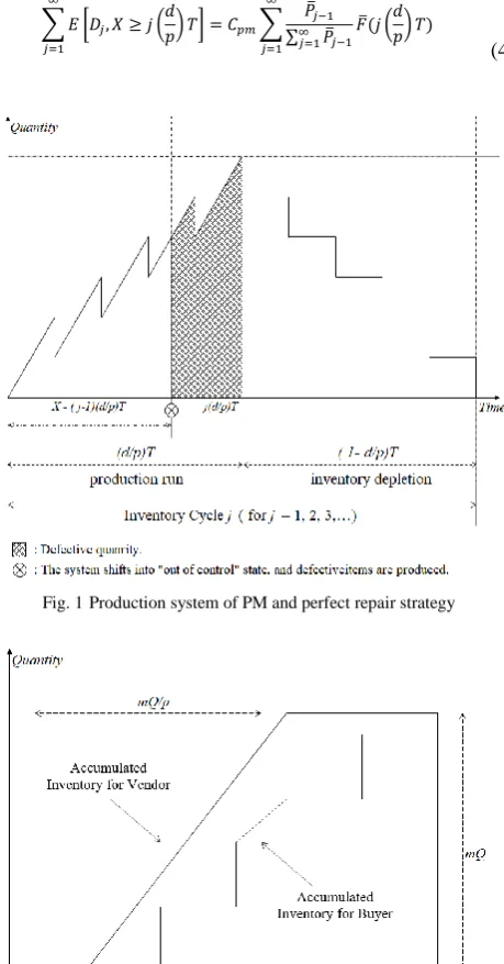
PM aims to reduce or eliminate unplanned downtime, thereby increasing machine efficiency. PM also helps to maintain a production system in optimal operating condition. Higher reliability increases the consistency of producing products with acceptable quality and performance characteristics (for example, MTBF) by avoiding production failures and ensuring product uniformity. Thus, it reduces costs associated with inspection, rework, and repair. To model the problem, the inventory cycle is separated into two periods [23]:
I. the inventory building period (production run period) II. the inventory depletion period (PM or repair period)
The Production system of PM and perfect repair strategy based on the general model is illustrated in Fig. 1, inventory model for vendor is illustrated in Fig. 2, and definition of notation of integrated model is shown on Table I. In last chapter, we show the necessary assumptions to develop the integrated inventory model for the joint determination of production, maintenance, and repair are as below:
A. Assumptions
1. There is only one type of product in the production system.
2. Production rate, demand rate, setup cost, ordering cost, and holding cost are known as constants. Backorder is not permitted.
TABLEI
DEFINITION OF NOTATION OF INTEGRATED MODEL
Notation Definition
T Time of an inventory cycle, 𝑇 = 𝑚𝑄/𝑑
X Cumulative production runtime to failure of a new system p Production rate in units per year
d Demand rate in units per year; 𝑝 > 𝑑 Q Order quantity of each delivery
m Integer number of lots of items delivered from vendor to purchaser in an inventory cycle
Ch Inventory cost rate per unit per year Cs Vendor’s setup cost for each production run Cv Vendor’s production cost per unit Co Purchaser’s ordering cost for each order Cp Purchaser’s purchase cost per unit Cpm Cost of each PM
Cr Perfect repair cost for each failure Ci Inspection cost of per unit Crw Rework cost of per unit
𝑃̅𝑗 Probability that the first j PMs are imperfect PMs; 𝑃̅0= 1
𝑞𝑗
Probability that the jth PM is an imperfect PM; 𝑞𝑗=
𝑃̅𝑗/𝑃̅𝑗−1
𝜃𝑗 Probability that the jth PM is a perfect PM; 𝜃𝑗= 1 − 𝑞𝑗
𝑝𝑗 Probability that PM is perfect following the (𝑗 − 1) imperfect PM; 𝑝𝑗= 𝑃̅𝑗−1𝜃𝑗= 𝑃̅𝑗−1− 𝑃̅𝑗
𝐹(𝑡) Failure distribution function of 𝑋
𝑓(𝑡) Failure density function associated with 𝐹(𝑡)
3. The term T denotes a whole inventory cycle, and further, it could be separated into two periods: a) (𝑑/𝑝)𝑇 represents the inventory building period
(production run period).
b) (1 − 𝑑/𝑝)𝑇 represents the inventory depletion period (PM period).
4. The original system begins to operate at time 0. The production process begins in an in-control state and conforming items are produced.
5. Setup cost Cs is incurred at the start of each inventory cycle.
6. The cost of each PM is Cpm. PM is performed
following the production run period. PM is performed at cumulative production runtime j(𝑑/𝑝)𝑇 for ( j = 1, 2, …). One of the following two cases results: a) Imperfect PM results in the unit having the same
failure rate as before PM, with probability 𝑞𝑗= 𝑃̅𝑗
𝑃̅𝑗−1 for(0 ≤ 𝑞𝑗≤ 1).
b) Perfect PM obtains an as-good-as-new units, with probability 𝜃𝑗= 1 − 𝑞𝑗.
7. If failure occurs, the system shifts into the
out-of-control state during which defective items are produced. Perfect repair, complete inspection, and rework are conducted after this run period. The term
Cr, Ci, Crw represent the perfect repair, inspection, and rework cost respectively.
8. After perfect repair or perfect PM, the system is as good as new. The system returns to age 0.
9. The time of PM or repair are not a constant, but it must be less than or equals to (1 − 𝑑/𝑝)𝑇.
If the jth instance of the PM is performed, then it is either
imperfect or perfect. Let X denotes the cumulative production runtime to a failure of a new system. For the present policy
(1) Where Uj represents the in-control production runtime during the jth inventory cycle after (j–1) imperfect PMs. As
mentioned earlier, we use the concept of an imperfect PM. Note that the probability after ( j–1) imperfect PMs is given by for ∑ 𝑃̅𝑗−1
𝑃̅𝑗−1 ∞
𝑗=1 for ( j = 1, 2, …). Thus, expected time of an in-control production run is:
(2)
B. Vendor’s Total Expected Cost
Let Dj denote the total PM and restoration costs during the
jth inventory cycle, including the restoration costs (inspection,
rework, and perfect repair costs) and the PM cost of the jth
PM. Furthermore, the expected PM and restoration costs for one inventory cycle are:
(3) PM is performed after the in-control production run period. That is, 𝑋 ≥ 𝑗 (𝑑
𝑝) 𝑇 for ( j = 1, 2, 3, …) following ( j–1) imperfect PMs. The expected PM cost is:
(4)
If the system is found to be out of control, restoration works are conducted after this production run period. Perfect repair action can restore the system operating condition to as
𝑈𝑗= {
𝑋 − (𝑗 − 1) (𝑑
𝑝) 𝑇, 𝑖𝑓 (𝑗 − 1) ( 𝑑
𝑝) 𝑇 < 𝑋 < 𝑗 ( 𝑑 𝑝) 𝑇
(𝑑
𝑝) 𝑇, 𝑖𝑓 𝑋 ≥ 𝑗 ( 𝑑 𝑝) 𝑇
for j = 1, 2, …
∑ 𝐸[𝑈𝑗] ∞
𝑗=1
= ∑ 𝑃̅𝑗−1 ∑∞𝑗=1𝑃̅𝑗−1 ∞
𝑗=1
× {∫ [t − (𝑗 − 1) (𝑑
𝑝) 𝑇] 𝑓(𝑡)𝑑𝑡 𝑗(𝑑𝑝)𝑇
(𝑗−1)(𝑑𝑝)𝑇 + (
𝑑 𝑝) 𝑇𝐹̅(𝑗(
𝑑 𝑝)𝑇)}
= ∑(𝑃̅𝑗−1− 𝑃̅𝑗) ∑∞𝑗=1𝑃̅𝑗−1 ∞
𝑗=1
∫ 𝐹̅(𝑡)𝑑𝑡
𝑗(𝑑𝑝)𝑇
0
∑ 𝐸[𝐷𝑗] ∞
𝑗=1
= ∑ 𝐸 [𝐷𝑗, 𝑋 ≥ 𝑗 (
𝑑 𝑝) 𝑇]
∞
𝑗=1
+ ∑ 𝐸 [𝐷𝑗, (𝑗 − 1) (
𝑑
𝑝) 𝑇 < 𝑋 < 𝑗 ( 𝑑 𝑝) 𝑇]
∞
𝑗=1
∑ 𝐸 [𝐷𝑗, 𝑋 ≥ 𝑗 (𝑑
𝑝) 𝑇] = 𝐶𝑝𝑚∑
𝑃̅𝑗−1
∑∞𝑗=1𝑃̅𝑗−1
𝐹̅(𝑗 (𝑑 𝑝) 𝑇)
∞
𝑗=1 ∞
𝑗=1
[image:3.595.312.542.227.666.2]Fig. 1Production system of PM and perfect repair strategy
[image:3.595.313.535.525.720.2]good as new. The defective items are observed by inspecting this lot. The process produces defective items only in the out-of-control state. The expected number of defective item is:
(5) All these defective products are reworked in the same cycle. The restoration costs are:
(6) = expected repair cost + expected inspection cost +
expected rework cost
(7) The inventory level of this model and production system is illustrated in Fig.2. Once vendor receives an order, vendor starts to produce immediately until the quantity reach to mQ. Products delivered from vendor to buyer by each Q unit, and there are m lots will deliver in an inventory cycle. The average inventory of vendor could be evaluated as following statement:
(8) According to the assumptions and notations, the total expected cost of vendor could be present as below:
TEC(v) = Setup Cost + Holding Cost + PM cost
+ Restoration costs 1) Setup cost: Cs
2) Holding Cost : 𝐶ℎ𝐶𝑣{𝑄2𝑚 [(1 −𝑑𝑝) − 1 +2𝑑𝑝]} 3) PM cost : 𝐶𝑝𝑚∑
𝑃̅𝑗−1 ∑∞𝑗=1𝑃̅𝑗−1𝐹̅(𝑗 (
𝑑 𝑝) 𝑇) ∞
𝑗=1
4) Restoration costs:
(𝐶𝑟+ 𝐶𝑖𝑇𝑑) ∑
𝑃̅𝑗−1 ∑∞𝑗=1𝑃̅𝑗−1 ∞
𝑗=1 𝐹((𝑑𝑝) 𝑇)
+ 𝐶𝑟𝑤𝑝 [(𝑑𝑝) 𝑇 − ∑
(𝑃̅𝑗−1−𝑃̅𝑗) ∑∞𝑗=1𝑃̅𝑗−1 ∞
𝑗=1 ∫ 𝐹̅(𝑡)𝑑𝑡
𝑗(𝑑𝑝)𝑇
0 ]
C. Purchaser’s Total Expected Cost
Let TEC(p) = Ordering Cost + Holding Cost, and the expected cost of purchaser could be present as below:
1) Ordering Cost : 𝑚𝐶𝑜 2) Holding Cost : 𝐶ℎ𝐶𝑝𝑄2
Cause 𝑇 = 𝑚𝑄/𝑑, so holding cost of purchaser could be rewritten as : 𝑇𝑑/2𝑚
D. Joint Expected Total Cost
Let’s combine TEC(v) with TEC(p), we could obtain the joint expected total cost in an inventory cycle as below:
(9) Let
∑ 𝑃̅𝑗−1 ∑∞𝑗=1𝑃̅𝑗−1𝐹̅(𝑗 (
𝑑 𝑝) 𝑇) ∞
𝑗=1 = A,
∑ 𝑃̅𝑗−1 ∑∞𝑗=1𝑃̅𝑗−1 ∞
𝑗=1 𝐹(𝑗 (𝑑𝑝) 𝑇) = 𝐵,
∑ (𝑃̅𝑗−1−𝑃̅𝑗) ∑∞𝑗=1𝑃̅𝑗−1 ∞
𝑗=1 ∫ 𝐹̅(𝑡)𝑑𝑡
𝑗(𝑑𝑝)𝑇
0 = 𝑍
Then JTEC(T) could be show as bellows:
(10) Let’s take first-order partial derivative of JTEC(T), we could get the optimal T* in an inventory cycle. Then let set the derivation to zero, we have:
(11)
Theorem 1: Let’s take second-order partial derivative, if equation (12) > 0, then there exists a finite and unique optimal solution T* that could minimizes JTEC
(T).
(12)
Proof. See Appendix 1.
IV. NUMERICALEXAMPLE
To illustrate the usage of the model, we present a simple case which applies the PM policy of Nakagawa [24] who used an imperfect PM model in which PM yields a system as bad as old with probability p and as good as new with probability 𝑃̅ = 1 − 𝑃. Based on this case, we presented three sensitivity analyses in this case and observed the variation by increase of number of shipments m. The general
𝑝 × (expected out-of-control production run time)
= 𝑝 [(𝑑𝑝) 𝑇 − ∑ (𝑃̅𝑗−1−𝑃̅𝑗) ∑∞𝑗=1𝑃̅𝑗−1 ∞
𝑗=1 ∫ 𝐹̅(𝑡)𝑑𝑡
𝑗(𝑑𝑝)𝑇
0 ]
∑ 𝐸 [𝐷𝑗, (𝑗 − 1) (
𝑑
𝑝) 𝑇 < 𝑋 < 𝑗 ( 𝑑 𝑝) 𝑇]
∞
𝑗=1
= (𝐶𝑟+ 𝐶𝑖𝑇𝑑) ∑
𝑃̅𝑗−1 ∑∞𝑗=1𝑃̅𝑗−1 ∞
𝑗=1 𝐹((
𝑑 𝑝) 𝑇)
+ 𝐶𝑟𝑤𝑝 {(𝑑𝑝) 𝑇 − ∑∞𝑗=1𝐸[𝑈𝑗]}
= (𝐶𝑟+ 𝐶𝑖𝑇𝑑) ∑
𝑃̅𝑗−1 ∑∞𝑗=1𝑃̅𝑗−1 ∞
𝑗=1 𝐹((𝑑𝑝) 𝑇)
+ 𝐶𝑟𝑤𝑝 [(𝑑𝑝) 𝑇 − ∑
(𝑃̅𝑗−1−𝑃̅𝑗) ∑∞𝑗=1𝑃̅𝑗−1 ∞
𝑗=1 ∫ 𝐹̅(𝑡)𝑑𝑡
𝑗(𝑑𝑝)𝑇
0 ]
𝐼𝑣 =
{[𝑚𝑄(𝑄𝑝+(𝑚−1)𝑄 𝑑)−
𝑚2𝑄2 2𝑝 ]−[
𝑄2
𝑑(1+2+⋯+(𝑚−1))]} (𝑚𝑄
𝑑)
=𝑄2𝑚 [(1 −𝑑𝑝) − 1 +2𝑑
𝑝]
𝐽𝑇𝐸𝐶(𝑇)=
𝑇𝑑
2𝑚(𝐶ℎ𝐶𝑝+ 𝐶ℎ𝐶𝑣{𝑚 [(1 −
𝑑 𝑝) − 1 +
2𝑑 𝑝]})
+ (1
𝑇)
{
𝐶𝑠+ 𝑚𝐶𝑜+ 𝐶𝑝𝑚∑ ∑∞𝑃̅𝑗−1𝑃̅𝑗−1 𝑗=1 𝐹̅(𝑗 (
𝑑 𝑝) 𝑇) ∞
𝑗=1
+ (𝐶𝑟+ 𝐶𝑖𝑇𝑑) ∑ ∑∞𝑃̅𝑗−1𝑃̅𝑗−1 𝑗=1 ∞
𝑗=1 𝐹(𝑗 (𝑑𝑝) 𝑇)
+ 𝐶𝑟𝑤𝑝 [(𝑑𝑝) 𝑇 − ∑ (𝑃̅𝑗−1−𝑃̅𝑗)∑∞ 𝑃̅𝑗−1 𝑗=1 ∞
𝑗=1 ∫ 𝐹̅(𝑡)𝑑𝑡
𝑗(𝑑𝑝)𝑇
0 ]}
𝑇𝑑
2𝑚(𝐶ℎ𝐶𝑝+ 𝐶ℎ𝐶𝑣{𝑚 [(1 − 𝑑 𝑝) − 1 +
2𝑑 𝑝]})
+ (𝑇1) {𝐶𝑠+ 𝑚𝐶𝑜+ 𝐶𝑝𝑚𝐴 + (𝐶𝑟+ 𝐶𝑖𝑇𝑑)𝐵 +
𝐶𝑟𝑤𝑝 [(𝑑𝑝) 𝑇 − 𝑍]}
𝑑
2𝑚(𝐶ℎ𝐶𝑝+ 𝐶ℎ𝐶𝑣{𝑚 [(1 − 𝑑 𝑝) − 1 +
2𝑑
𝑝]}) + 𝐶𝑖𝑑𝐵 ′
+ (𝑇12) [ −𝐶𝑠− 𝑚𝐶𝑜+ 𝐶𝑝𝑚(−𝐴 + 𝑇𝐴′) +𝐶𝑟(−𝐵 + 𝑇𝐵′) + 𝐶𝑟𝑤𝑝(𝑍 − 𝑇𝑍′)] = 0
𝐶𝑖𝑑𝐵′′+
(𝑇13) [
𝐶𝑠+ 𝑚𝐶𝑜+ 𝐶𝑝𝑚(𝐴 − 2𝑇𝐴′+ 𝑇2𝐴′′)
+𝐶𝑟(𝐵 − 2𝑇𝐵′+ 𝑇2𝐵′′)
+𝐶𝑟𝑤𝑝(−𝑍 + 2𝑇𝑍′− 𝑇2𝑍′′)
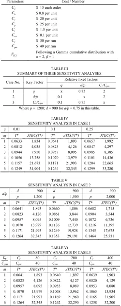
variables setting were shown in table II, and setting of key factors for every sensitivity analysis cases were shown in table III. The outcomes of three sensitivity analyses cases were shown on table IV-VI:
From the sensitivity analysis of the numerical example (Tables IV–VI), the following results are obtained.
1. For all cases of sensitivity analyses, the total cost rise sharp by increasing of integer number of shipments m.
2. For sensitivity analysis in case 1, the total cost and the optimal T* rise by increasing of probability of imperfect PM q.
3. For sensitivity analysis in case 2, the total cost rise by increasing of ratio of d/p. By contrast, the optimal
T* rise by decreasing of ratio of d/p.
4. For sensitivity analysis case 3, the total cost rise by increasing of proportion of Cr/Cpm when the integer number of shipment m is small (where m > 3 in this case), While the integer number of shipment m is getting larger, the total cost decrease by growth of proportion of of Cr/Cpm. Whereas, the optimal T*
descends simply by increasing of proportion of
Cr/Cpm.
5. Comparing the outcomes of three sensitivity analyses, sensitivity of total cost is relative high by variation of ratio of d/p. where the other are not. 6. For perspectives of managers in businesses, number
of shipments m, and production rate and demand rate may be the most important factors when they apply this model for the real production work.
V. CONCLUSIONS
This paper demonstrated that enhancing maintenance and production capabilities increases the reliability of goods, thereby reducing whole inventory costs. The rule of economies of scale was shown obviously in this model where total inventory cost rose by increasing of integer number of shipments m. Product reliability and product uniformity must be incorporated into equipment operating conditions to increase the production policy dependency on the maintenance program. Historical maintenance data can be used to determine failure trends and probability 𝑃̅𝑗, and the integrated inventory model can assist policy-makers in making appropriate decisions related to PM and production plans.
In order to test the performance and application of the integrated inventory model initially, this paper did not combine the setting of free-repair warranty from Liao [1]. Future studies can address problems to mixed this idea and relax the restrictions of this paper, such as allowing for shortages and imperfect inspections during the out-of-control state.
APPENDIX Proof of Theorem 1:
Let 𝑄(𝑇) be the left-hand side of equation (10) in origin form:
TABLEII
GENERALSETTINGOFTHREESENSITIVITYANALYSES
Parameters Cost / Number
Co $ 15 each order Ch $ 0.8 per unit Cv $ 20 per unit Cp $ 25 per unit Ci $ 1.5 per unit Crw $ 0.1 per unit Cs $ 30 per run Cpm $ 40 per run
𝐹(𝑡) Following a Gamma cumulative distribution with
α = 2, β = 1
TABLEIII
SUMMARYOFTHREESENSITIVITYANALYSES
Case No. Key Factor Relative fixed factors
q d/p Cr/Cpm
1 q x 0.75 2
2 d/p 0.1 x 2
3 Cr/Cpm 0.1 0.75 x
Where p = 1200; d = 900 for d/p = 0.75 in this table.
TABLEIV
SENSITIVITY ANALYSIS IN CASE 1
q 0.01 0.1 0.25
m T* JTEC(T*) T* JTEC(T*) T* JTEC(T*)
1 0.0633 1,834 0.0641 1,893 0.0657 1,992 2 0.0812 4,035 0.0823 4,126 0.0847 4,297 3 0.0944 7,950 0.0957 8,095 0.0985 8,385 4 0.1056 13,758 0.1070 13,979 0.1101 14,436 5 0.1157 21,673 0.1171 21,993 0.1204 22,665 6 0.1249 31,904 0.1264 32,345 0.1299 33,280
TABLEV
SENSITIVITY ANALYSIS IN CASE 2
d/p d 900 d ,900 d 900
p 1,200 p 1,500 p 2,000
m T* JTEC(T*) T* JTEC(T*) T* JTEC(T*)
1 0.0641 1,893 0.0660 1,806 0.0682 1,715 2 0.0823 4,126 0.0861 3,844 0.0904 3,544 3 0.0957 8,095 0.1009 7,440 0.1072 6,736 4 0.1070 13,979 0.1136 12,739 0.1216 11,395 5 0.1171 21,993 0.1249 19,928 0.1345 17,675 6 0.1264 32,345 0.1353 29,191 0.1464 25,731
TABLEVI
SENSITIVITY ANALYSIS IN CASE.3
𝐶𝑟
𝐶𝑝𝑚
Cr 80 Cr 200 Cr 400
Cpm 40 Cpm 40 Cpm 40
m T* JTEC(T*) T* JTEC(T*) T* JTEC(T*)
[image:5.595.46.297.131.762.2]∑∞𝑗=1𝑃̅𝑗[𝑗 (𝑑𝑝) 𝑇𝑓(𝑗 (𝑑𝑝) 𝑇)(𝐶𝑟− 𝐶𝑝𝑚+ 𝐶𝑖𝑇𝑑)]
− ∑∞𝑗=1𝑃̅𝑗−1[𝐹̅(𝑗 (𝑑𝑝) 𝑇)𝐶𝑝𝑚+ 𝐹(𝑗 (𝑑𝑝) 𝑇)𝐶𝑟] +
∑∞𝑗=1(𝑃̅𝑗−1− 𝑃̅𝑗)𝐶𝑟𝑤𝑝 [∫ 𝐹̅(𝑡)𝑑𝑡 𝑗(𝑑𝑝)𝑇
0 − 𝑗 (
𝑑
𝑝) 𝑇𝐹̅(𝑗 ( 𝑑 𝑝) 𝑇)]
is strictly increasing in (𝑑
𝑝) 𝑇, 𝑄(0) < 0 and 𝑄(∞) > 0
𝑄(𝑇) is strictly increasing from −𝐶𝑠− 𝑚𝐶𝑜 to ∞. Thus, there exists a unique and finite T*, (0 < T* < ∞) satisfying equation (10), which could minimize JTEC(T).
REFERENCES
[1] G.-L. Liao, “Production and Maintenance Policies for an EPQ Model with Perfect Repair, Rework, Free-Repair Warranty, and Preventive Maintenance,” IEEE T SYST MAN CY-S, vol. 46, no. 8, pp. 1129–1139, August 2016.
[2] M.-F. Yang and Y. Lin, “Integrated inventory model with backorder and minimal repair in a supply chain,” P I MECH ENG B-J ENG, pp. 1–15, May 2016.
[3] F. Harris, “How many parts to make at once?” Factory, the Magazine of Management, vol. 10, no. 2, pp. 135–136, Feb. 1913.
[4] D. Das, A. Roy, and S. Kar, “A volume flexible economic production lot-sizing problem with imperfect quality and random machine,” J. Comput. Math. Appl., vol. 61, no. 9, pp. 2388–2400, May 2011. [5] B. Pal, S. S. Sana, and K. Chaudhuri, “Maximizing profits for an EPQ
model with unreliable machine and rework of random defective items,” Int. J. Syst. Sci., vol. 44, no. 3, pp. 582–594, 2013.
[6] H.-M. Wee, W.-T. Wang, and P.-C. Yang, “A production quantity model for imperfect quality items with shortage and screening constraint,” Int. J. Prod. Res., vol. 51, no. 6, pp. 1869–1884, 2013. [7] G.-L. Liao, “Optimal production correction and maintenance policy for
imperfect process,” Eur. J. Oper. Res., vol. 182, no. 3, pp. 1140–1149, Nov. 2007
[8] R. Barlow and L. Hunter “Optimum preventive maintenance policies,” Oper. Res., pp. 90–100, 1959.
[9] C. R. Cassady and E. Kutanoglu, “Integrating preventive maintenance planning and production scheduling for a single machine,” IEEE Trans. Rel., vol. 54, no. 2, pp. 193–199, Jun. 2005.
[10] R. I. Zequeira and C. Berenguer, “Periodic imperfect preventive maintenance with two categories of competing failure modes,” Reliab. Eng. Syst. Safe., vol. 91, no. 4, pp. 460–468, Apr. 2006.
[11] S.-H. Sheu and C.-C. Chang, “An extended periodic imperfect preventive maintenance model with age-dependent failure type,” IEEE Trans. Rel., vol. 58, no. 2, pp. 397–405, Jun. 2009.
[12] X. Lu, M. Chen, M. Liu, and D. Zhou, “Optimal imperfect periodic preventive maintenance for systems in time-varying environments,” IEEE Trans. Rel., vol. 61, no. 2, pp. 426–439, Jun. 2012.
[13]D. Lin, M. Zuo, and R. Yam, “Sequential imperfect preventive maintenance models with two categories of failure modes,” Naval Res. Logist., vol. 48, no. 2, pp. 172–183, Mar. 2001.
[14] J. Schutz, N. Rezg, and J.-B. Léger, “Periodic and sequential preventive maintenance policies over a finite planning horizon with a dynamic failure law,” J. Intell. Manuf., vol. 22, no. 4, pp. 523–532, Aug. 2011.
[15] S. Ayed, S. Sofiene, and R. Nidhal, “Joint optimization of maintenance and production policies considering random demand and variable,” Int. J. Prod. Res., vol. 50, no. 23, pp. 6870–6885, 2012.
[16] E. Y. Lee and J. Lee, “An optimal proportion of perfect repair,” Oper. Res. Lett., vol. 25, no. 3, pp. 147–148, Oct. 1999.
[17] L. Cui, W. Kuo, H. T. Loh, and M. Xie, “Optimal allocation of minimal & perfect repairs under resource constraints,” IEEE Trans. Rel., vol. 53, no. 2, pp. 193–199, Jun. 2004.
[18] S.K. Goyal,“An integrated inventory model for a single supplier single customer problem,” Int. J. Prod. Res., pp. 107–111, 1976.
[19] R.V. Ramasesh, “Recasting the traditional inventory model to implement just-in-time purchasing,” Prod. Inventory. Manag. J., pp. 71–75, Jan. 1990.
[20] J.C. Martinich, Production and operations management. New York: Wiley, 1997.
[21] A. Banerjee, “A joint economic-lot-size model for purchaser and vendor,” Decision Science, vol. 17, no. 3, pp. 292–311, Jul. 1986. [22] D. Ha and S.-L. Kim, “Implementation of JIT purchasing: an integrated
approach,” Prod Plan Control, vol. 8, no. 2, pp. 152–157, 1997. [23] G.-L. Liao, “Joint production and maintenance strategy for economic
production quantity model with imperfect production processes,” J. Intell. Manuf., vol. 24, no. 6, pp. 1229–1240, Dec. 2013.
[24] T. Nakagawa, “Optimum policies when preventive maintenance is imperfect,” IEEE Trans. Rel., vol. R-28, no. 4, pp. 331–332, Oct. 1979.
𝑄(𝑇) =2𝑚𝑑 (𝐶ℎ𝐶𝑝+ 𝐶ℎ𝐶𝑣{𝑚 [(1 −𝑑𝑝) − 1 +2𝑑𝑝]}) + 1
𝑇(𝐶𝑟+ 𝐶𝑖𝑇𝑑 −
𝐶𝑝𝑚) ∑ 𝑃̅𝑗 ∑∞𝑗=1𝑃̅𝑗𝑗 (
𝑑 𝑝) 𝑓(𝑗 (
𝑑 𝑝) 𝑇) ∞
𝑗=1 +
1
𝑇2{−𝐶𝑠− 𝑚𝐶𝑜−
𝐶𝑝𝑚∑
𝑃̅𝑗−1 ∑∞𝑗=1𝑃̅𝑗−1𝐹̅(𝑗 (
𝑑 𝑝) 𝑇) ∞
𝑗=1 −
𝐶𝑟∑
𝑃̅𝑗−1 ∑∞𝑗=1𝑃̅𝑗−1 ∞
𝑗=1 𝐹(𝑗 (𝑑𝑝) 𝑇) +
𝐶𝑟𝑤𝑝 [∑
(𝑃̅𝑗−1−𝑃̅𝑗) ∑∞𝑗=1𝑃̅𝑗−1 ∞
𝑗=1 ∫ 𝐹̅(𝑡)𝑑𝑡
𝑗(𝑑𝑝)𝑇
0 −
∑ (𝑃̅𝑗−1−𝑃̅𝑗) ∑∞𝑗=1𝑃̅𝑗−1𝑗 (
𝑑 𝑝) ∞
𝑗=1 𝑇𝐹̅(𝑗 (
𝑑 𝑝) 𝑇)]}
= −𝐶𝑠− 𝑚𝐶𝑜+𝑇 2𝑑
2𝑚(𝐶ℎ𝐶𝑝+ 𝐶ℎ𝐶𝑣{𝑚 [(1 − 𝑑
𝑝) − 1 + 2𝑑
𝑝]}) + (𝐶𝑟− 𝐶𝑝𝑚+
𝐶𝑖𝑇𝑑) ∑ 𝑃̅𝑗 ∑∞𝑗=1𝑃̅𝑗𝑗 (
𝑑 𝑝) 𝑇𝑓(𝑗 (
𝑑 𝑝) 𝑇) ∞
𝑗=1 −
𝐶𝑝𝑚∑
𝑃̅𝑗−1 ∑∞𝑗=1𝑃̅𝑗−1𝐹̅(𝑗 (
𝑑 𝑝) 𝑇) ∞
𝑗=1 −
𝐶𝑟∑
𝑃̅𝑗−1 ∑∞𝑗=1𝑃̅𝑗−1 ∞
𝑗=1 𝐹(𝑗 (𝑑𝑝) 𝑇) +
𝐶𝑟𝑤𝑝 [∑
(𝑃̅𝑗−1−𝑃̅𝑗) ∑∞𝑗=1𝑃̅𝑗−1 ∞
𝑗=1 ∫ 𝐹̅(𝑡)𝑑𝑡
𝑗(𝑑𝑝)𝑇
0 −
∑ (𝑃̅𝑗−1−𝑃̅𝑗) ∑∞𝑗=1𝑃̅𝑗−1𝑗 (
𝑑 𝑝) ∞
𝑗=1 𝑇𝐹̅(𝑗 (𝑑𝑝) 𝑇)]
𝑄(0) = −𝐶𝑠− 𝑚𝐶𝑜 < 0