Identification Of Temporal Dynamics Of Vegetation Coverage Using Remote Sensing And Gis (A Case Study Of Western Part Of West Bengal, India)

(1)

Identification Of Temporal Dynamics Of Vegetation Coverage Using Remote Sensing And Gis (A

Case Study Of Western Part Of West Bengal, India)

1

_{Gouri Sankar Bhunia and}

1

_{Rajendra Memorial Research Institutes of Medical Sciences (ICMR), Agamkuan, Patna}

2

_{Department of Geography and Environment Management, Vidyasagar University,}

Medinipur

ARTICLE INFO ABSTRACT

Monitoring vegetation coverage changes using multi evaluation of anthropogenic

spatio-temporal changes in vegetation cover using the potential multi 2002, 2005 and 2009 in Kangswati (Cossi) river and Dw

changes were determined using image differencing of normalized difference vegetation index (NDVI) in that time series. The highest maximum NDVI value was found in 2009 (maximum NDVI of 0.99), and lowe

recorded in 1999 (maximum NDVI of 0.48). By 2002

and in 2009, it grew to 1.03%. In 2002 and 2005, highest percent of surface area is coved with the low density vegetation zone. By 1999

was an increased in trend. Between 1999 and 2009, the low density vegetation zone portrayed increased in trend. Assessment conducted on the generated thematic images sign

However, the NDVI results indicated the vegetated area decreased and it may be due to the anthropogenic intervention.

INTRODUCTION

Vegetation or forest is the most important factors governing the ecology of an area, providing inferences to derive parameters like land use, water table, soil information etc (Bakr et al., 2010). Forest and wild life are essential biological components for maintaining the ecological balance of a geographical area. The importance of mapping, quantifying, and monitoring changes in the physical characteristics of forest cover has been widely recognized as a key element in the study of global change (Nemani and

The vegetation mapping is to recognize and characterize the different vegetation cover on the earth surface and it appraises particular vegetation characteristics and its coverage. The change in vegetation pattern has a feedback influence on the local and regional climate by reducing evaporative water losses from surface to atmosphere.

Study of vegetation characteristics over a long time periods of an area provide an inimitable opportunity to recognize vegetation dynamics, including interannual variability in vegetation composition and spatial changes (Rahman et al., 2011; Pen˜ uelas et al., 2007; Root 2003). A difficulty often encountered in vegetation resource mapping is of demarcation of plant cover from other varieties of veget

bushes, agriculture, etc., when they are stirring contiguously or in the locality (Neldner et al., 2012; Chastan et al., 2006). However, the reflectance pattern from tree cover and soft stem vegetation like agriculture crops illustrates emblematic tones on the satellite imagery due to topographical and phonological variations. Consequently, because of occurrences of vegetation characteristics of transitional gradations, severance of tree vegetation from bushy or herbaceous vegetation becomes tricky. Digitally processing of remote sensing data provides tools for investigating the satellite data through various

*Corresponding author:[email protected]

ISSN: 0975-833X

International Journal of Current Research

Vol.

Article History:

Received 07th

December, 2012 Received in revised form 28th

January, 2013 Accepted 24th

February, 2013 Published online 19th

March, 2013 Key words: Vegtation coverage, Spatio-temporal, NDVI, Change detection.

RESEARCH ARTICLE

Identification Of Temporal Dynamics Of Vegetation Coverage Using Remote Sensing And Gis (A

Of Western Part Of West Bengal, India)

Gouri Sankar Bhunia and Pravat Kumar Shit

Rajendra Memorial Research Institutes of Medical Sciences (ICMR), Agamkuan, Patna-800007, Bihar, India

Department of Geography and Environment Management, Vidyasagar University,

Medinipur-721102, West Bengal, India

ABSTRACT

Monitoring vegetation coverage changes using multi-temporal remotely-sensed data offers an efficient and exact evaluation of anthropogenic intervention on the natural environment. Study was conducted to explore the temporal changes in vegetation cover using the potential multi-temporal satellite data captured in 1999, 2002, 2005 and 2009 in Kangswati (Cossi) river and Dwarakeswar river interfluves area, West Bengal. Temporal changes were determined using image differencing of normalized difference vegetation index (NDVI) in that time series. The highest maximum NDVI value was found in 2009 (maximum NDVI of 0.99), and lowe

recorded in 1999 (maximum NDVI of 0.48). By 2002 - 2005, the area of surface waterbody decreased to 0.89% and in 2009, it grew to 1.03%. In 2002 and 2005, highest percent of surface area is coved with the low density vegetation zone. By 1999 – 2005, there was decreased in trend of bare surface area, while in 2005

was an increased in trend. Between 1999 and 2009, the low density vegetation zone portrayed increased in trend. Assessment conducted on the generated thematic images signifies accuracies of 86.0%

However, the NDVI results indicated the vegetated area decreased and it may be due to the anthropogenic intervention.

Copyright, IJCR, 2013, Academic Journals

Vegetation or forest is the most important factors governing the ecology of an area, providing inferences to derive parameters like land ., 2010). Forest and r maintaining the ecological balance of a geographical area. The importance of mapping, quantifying, and monitoring changes in the physical characteristics of forest cover has been widely recognized as a key Running, 1996). The vegetation mapping is to recognize and characterize the different vegetation cover on the earth surface and it appraises particular vegetation characteristics and its coverage. The change in vegetation on the local and regional climate by reducing evaporative water losses from surface to atmosphere.

Study of vegetation characteristics over a long time periods of an area provide an inimitable opportunity to recognize vegetation dynamics, annual variability in vegetation composition and spatial ., 2007; Root et al., 2003). A difficulty often encountered in vegetation resource mapping is of demarcation of plant cover from other varieties of vegetation like bushes, agriculture, etc., when they are stirring contiguously or in the ., 2006). However, the reflectance pattern from tree cover and soft stem vegetation like ic tones on the satellite imagery due to topographical and phonological variations. Consequently, because of occurrences of vegetation characteristics of transitional gradations, severance of tree vegetation from bushy or herbaceous ky. Digitally processing of remote sensing data provides tools for investigating the satellite data through various

[email protected]

algorithms and mathematical indices of spectral bands (Roy and Ravan, 1996; Goslee, 2011). Based on the reflectance properties, indices have been formulated to emphasize features of interest on the remote sensing data. There are numerous indices for accent vegetation-bearing areas on a satellite data, and Normalized Difference Vegetation Index (NDVI) is a general and extensively used

index (Yin et al., 2012; Joshi, 2011; Drissi

1985). Several change detection studies have shown

changes in vegetation properties are best identified when image data are enhanced using vegetation indices prior to image differencing (Coppin and Bauer, 1996; Fung, 1990; Mas, 1999; Radeloff 2000).

Assessment of vegetation vigour with remotely sensed imagery has been fairly triumphant. Both mechanistic and experimental methods are extensively employed in modeling vegetation dynamics (Carmel

et al., 2001; Qi et al., 2000). The vegetation mapping is to recognize and characterize the different vegetation cover on the earth surface and it appraises particular vegetation characteristics and its coverage. The change in vegetation pattern has a feedback influence on the local and regional climate by reducing evaporative water losses fro surface to atmosphere. In the present study, we explored the spatio temporal changes in vegetation cover using the potential multi temporal satellite data in Kangswati (Cossi) river and Dwarakeswar river interfluves area, West Bengal (India).

Study area

The study area is extended between 23°12´44.87˝

latitude and 86°50´06.83˝ E to 87°49´49.65˝

area of 7,512.62 km2. The present study represents regional diversities

in terms of physiographic, agro-climatic char development and social composition etc. region can be categorized into three parts, ternational Journal of Current Research

Vol. 5, Issue, 03, pp. 652-658, March,2013

INTERNATIONAL

OF CURRENT RESEARCH

Identification Of Temporal Dynamics Of Vegetation Coverage Using Remote Sensing And Gis (A

800007, Bihar, India

Department of Geography and Environment Management, Vidyasagar University,

sensed data offers an efficient and exact intervention on the natural environment. Study was conducted to explore the

temporal satellite data captured in 1999, arakeswar river interfluves area, West Bengal. Temporal changes were determined using image differencing of normalized difference vegetation index (NDVI) in that time series. The highest maximum NDVI value was found in 2009 (maximum NDVI of 0.99), and lowest value was 2005, the area of surface waterbody decreased to 0.89% and in 2009, it grew to 1.03%. In 2002 and 2005, highest percent of surface area is coved with the low density 2005, there was decreased in trend of bare surface area, while in 2005 – 2009, there was an increased in trend. Between 1999 and 2009, the low density vegetation zone portrayed increased in trend. ifies accuracies of 86.0%–92.0% were attained. However, the NDVI results indicated the vegetated area decreased and it may be due to the anthropogenic

algorithms and mathematical indices of spectral bands (Roy and Ravan, 1996; Goslee, 2011). Based on the reflectance properties, indices have been formulated to emphasize features of interest on the remote sensing data. There are numerous indices for accent bearing areas on a satellite data, and Normalized Difference Vegetation Index (NDVI) is a general and extensively used ., 2012; Joshi, 2011; Drissi et al., 2009; Justice et al., 1985). Several change detection studies have shown that inter-date changes in vegetation properties are best identified when image data are enhanced using vegetation indices prior to image differencing

Bauer, 1996; Fung, 1990; Mas, 1999; Radeloff et al.,

with remotely sensed imagery has been fairly triumphant. Both mechanistic and experimental methods are extensively employed in modeling vegetation dynamics (Carmelm

The vegetation mapping is to recognize he different vegetation cover on the earth surface and it appraises particular vegetation characteristics and its coverage. The change in vegetation pattern has a feedback influence on the local and regional climate by reducing evaporative water losses from surface to atmosphere. In the present study, we explored the spatio-temporal changes in vegetation cover using the potential multi-temporal satellite data in Kangswati (Cossi) river and Dwarakeswar river interfluves area, West Bengal (India).

s extended between 23°12´44.87˝ N to 22°22´01.09˝ N

to 87°49´49.65˝ E longitude, and with an

. The present study represents regional diversities climatic characteristics, economic nt and social composition etc. Physiographically, of the

region can be categorized into three parts, viz Chotonagpur flanks

(2)

with hills, mounds and rolling lands in the western part, Rahr Plain with lateritic uplands in the middle part and alluvial plain of the east with recent deposits. The area is drained by the Dwarkeswar, Silabati, Kangsawati river. Drought-affected dry areas have found in the west but the eastern part is characterized by highly wet flood-affected areas. Dense dry deciduous forest in the west is replaced by semi-aquatic vegetations of marsh lands in the east.

MATERIALS AND METHODS

Image acquisition and processing

Landsat 4 and 5 imageries were used for this present study. Four periods of satellite data were selected to extract the vegetation vigor of the study area: Landsat-4 Thematic Mapper (TM) November 06, 1999; Landsat-5 TM October 29, 2002; November 14, 2005 and November 18, 2009. The details of the data were described in Table 1. All these images were rectified to Universal Transverse Mercator (UTM) coordinate system, Datum World Geodetic System (WGS) 84, Zone 45 North and based on second order Nearest Neighbour algorithm for matching the geographic projection of the reference data. The images were subtracted based on the Area of Interest (AOI) of the Kangswati and Dwarakeswar river interfluves area for further analysis.

Normalized Difference Vegetation Index (NDVI)

Green and vigorous vegetation reflects lesser amount of solar radiation in the visible wavelength (Channel3) contrasted to those in

near-infrared spectrum (Channel4). The Normalized Difference

Vegetation Index (NDVI) is defined by Rouse et al., (1974) and

Tucker (1979) as: NDVI = (Channel4 – Channel3) / (Channel4 +

Channel3). Four NDVI continuous images, for all dates, resulted from

this step with float data type (continuous real numbers). Each image at each date was recoded to only two values: 0 and 1. Zero for the non-vegetated land and one for non-vegetated land. The healthy and intense vegetation demonstrate a large and positive NDVI. In compare,

clouds, water and snow have better visible reflectance than those of near-infrared (NIR). Accordingly, those features acquiesces negative index values. Rock and bare soil enclosed areas have comparable reflectance in the VIS/NIR bands and consequence in vegetation indices near zero. Because of these possessions, NDVI has suit the principal tool for mapping changes in vegetation cover and analysis of the impacts of environmental phenomena.

The colour density slicing technique was pertained to the data provided by the NDVI images in order to codify the classes and compare vegetation changes of the interfluves areas and its surroundings in 1999 and 2009.

Change detection analysis

Alteration in canopy cover or vegetation biomass can be perceived by analyzing NDVI values between separated dates using image differencing. It entails subtracting one date of original or transformed (e.g. vegetation indices) imagery from a second date that has been precisely registered to the first (Banner and Lynham, 1981; Serneels

et al., 2001). It is normally carried out on the basis of gray values. The altered region and unchanged region is established by choosing the appropriate threshold values of gray levels in the difference image. The gray value of the difference image illustrates the changes of corresponding pixels of two images.

DIF [1999, 2000] =NDVI [1999] – NDVI [2000] DIF [2000, 2005] =NDVI [2000] – NDVI [2005] DIF [2005, 2009] =NDVI [2005] – NDVI [2009] DIF [1999, 2009] =NDVI [1999] – NDVI [2009]

Accuracy assessment

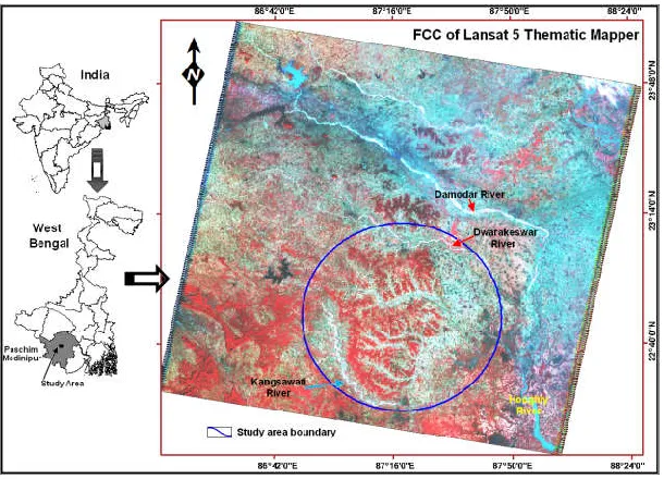
[image:2.612.157.462.126.346.2]

Accuracy of the vegetation coverage area was established empirically, by autonomously picking fifty random samples of pixels from each resulting map, from each technique at each date, and examining their labels aligned with classes dogged from reference data. The results of the analyses were articulated in an error matrix table, previously

Figure 1. Map of the study area

Table 1. Details characteristics of satellite data

Date of acquisition Scene ID Sensor Sun Azimuth Sun Elevation Spatial resolution

Cloud cover Geometric RMSE 06th November 1999 LE71390441999310SGS00 ETM+ 146.72 47.40 30 m 0.00 2.623

29th October 2002 LE71390442002302SGS00 ETM+ 150.09 45.90 30 m 0.00 3.655 14th November 2005 LT51390442005318BKT00 TM 150.22 43.21 30 m 2.00 4.432 25th November 2009 LT51390442009329KHC00 TM 151.68 40.93 30 m 0.00 4.026

[image:2.612.63.549.555.614.2]

(3)

offered by Congalton (1991). Kappa coefficient is also calculated to measure the map accuracy (Congalton and Green, 1999).

RESULTS AND DISCUSSION

NDVI analysis results

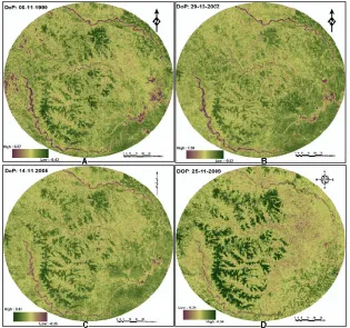
[image:3.612.148.463.239.534.2]

NDVI images was created using Landsat TM and ETM+ data for each image at each date (1999, 2002, 2005 and 2009) using band 3 (R) and band 4 (NIR) and used in the analysis of variation in NDVI. Vegetation index and difference images were generated for the 1 years study period (Figure 2a). Results showed that the vegetation index map derived by NDVI transformation within each computational group were dissimilar in terms of spatial distributional pattern and statistical characteristics. The highest maximum ND value was found in 2009, and lowest value was recorded in 1999. The mean NDVI value of the study area is gradually increasing during the period between 1999 and 2009 (Figure 2b).

Figure 2. Vegetation characteristics derived through NDVI at different period in the study area

Figure 2a. Temporal coverage of vegetation characteristics duri

offered by Congalton (1991). Kappa coefficient is also calculated to map accuracy (Congalton and Green, 1999).

NDVI images was created using Landsat TM and ETM+ data for each image at each date (1999, 2002, 2005 and 2009) using band 3 (R) and band 4 (NIR) and used in the analysis of variation in NDVI. Vegetation index and difference images were generated for the 10 years study period (Figure 2a). Results showed that the vegetation index map derived by NDVI transformation within each computational group were dissimilar in terms of spatial distributional pattern and statistical characteristics. The highest maximum NDVI value was found in 2009, and lowest value was recorded in 1999. The mean NDVI value of the study area is gradually increasing during the

Vegetation characteristics derived through NDVI at different

Monitoring spatial and temporal changes of vegetation coverage

The NDVI values were divided into seven main classes: surface waterbody, bare surface, very low density vegetation zone, low density vegetation zone, medium density vegetation zone, high density vegetation zone and very high density vegetation zone. negative values of NDVI represented the surface waterbody, and the value between 0.01 and 0.100 represented bare surface. However, the positive values of 0.101 – 0.250, represented agricultural/crop land, while the higher positive value represented the vege

Figure 2a and Table 2 explain the NDVI continuous images and the area coverage for the NDVI classes by square kilometer and percentage on different dates, respectively. Results showed that in 1999, the interfluves area were 44.70% (3358.28 km

(2537.28 km2) very low density vegetation zone and low density

vegetation zone respectively. By 2002 waterbody decreased to 0.89% (66.72km

1.03% (77.57km2). In 2002 and 2005, highest perc

is coved with the low density vegetation zone (44.15% and 41.28% respectively). By 2009, very low density vegetation zone increased to

59.54% (4472.68 km2_{), while the low density vegetation zone}

decreased (13.56%, 1018.50 km2). High density vegetation zone is

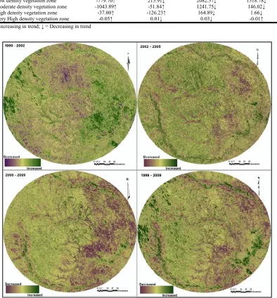
also decreased in 2009. However, very less percent of area covered with the very high density vegetation zone in the study site. According to the preceding results from the NDVI analysis, monitoring the alterations of vegetation converges between two dates were delineated. Table 3 and Figure 3a show the incessant vegetation coverage transform images using the outputs of NDVI analysis at two different dates and the differences between the are

from one land cover class to another by areas, respectively. The results showed that in 1999 and 2005, interfluves area of 153.21km

and 122.41km2 were decreased in surface waterbody; while in 2005

2009, 10.85 km2 _{areas were increased. H}

during the period between 1999 and 2009 showed decreased in trend

Temporal coverage of vegetation characteristics during the period from 1999 to 2009

Monitoring spatial and temporal changes of vegetation coverage

The NDVI values were divided into seven main classes: surface waterbody, bare surface, very low density vegetation zone, low density vegetation zone, medium density vegetation zone, high density vegetation zone and very high density vegetation zone. The egative values of NDVI represented the surface waterbody, and the value between 0.01 and 0.100 represented bare surface. However, the 0.250, represented agricultural/crop land, while the higher positive value represented the vegetated areas. Figure 2a and Table 2 explain the NDVI continuous images and the area coverage for the NDVI classes by square kilometer and percentage on different dates, respectively. Results showed that in

1999, the interfluves area were 44.70% (3358.28 km2_{) and 33.77%}

) very low density vegetation zone and low density vegetation zone respectively. By 2002 - 2005, the area of surface

waterbody decreased to 0.89% (66.72km2) and in 2009, it grew to

). In 2002 and 2005, highest percent of surface area

density vegetation zone (44.15% and 41.28% respectively). By 2009, very low density vegetation zone increased to

), while the low density vegetation zone ). High density vegetation zone is also decreased in 2009. However, very less percent of area covered with the very high density vegetation zone in the study site. According to the preceding results from the NDVI analysis,

onitoring the alterations of vegetation converges between two dates were delineated. Table 3 and Figure 3a show the incessant vegetation coverage transform images using the outputs of NDVI analysis at two different dates and the differences between the areas which changed from one land cover class to another by areas, respectively. The

results showed that in 1999 and 2005, interfluves area of 153.21km2

were decreased in surface waterbody; while in 2005 – areas were increased. However, the overall analysis during the period between 1999 and 2009 showed decreased in trend

[image:3.612.62.299.565.693.2]

(4)

[image:4.612.67.547.70.173.2]

Table 2. Surface characteristics of vegetation vigor derived through NDVI

Surface Characteristics NDVI Value

1999 2002 2005 2009

Area

(sq. km) Percent

Area (sq. km) Percent

Area (sq. km) Percent Surface waterbody <0.00 342.34 4.56 189.13 2.52 66.72 0.89 77.57 1.03 Bare surface 0.01 - 0. 100 598.28 7.96 337.85 4.50 291.83 3.88 1415.07 18.84 Very low density vegetation zone 0.101 -0. 250 3358.28 44.70 1911.25 25.44 2117.48 28.19 4472.68 59.54 Low density vegetation zone 0.251 - 0.350 2537.28 33.77 3316.98 44.15 3101.07 41.28 1018.50 13.56 Moderate density vegetation zone 0.351 - 0.450 669.72 8.91 1713.61 22.81 1765.45 23.50 523.70 6.97 High density vegetation zone 0.451 - 0.550 6.76 0.09 43.76 0.58 169.99 2.26 5.10 0.07 Very High density vegetation zone >0.551 0.01 0.00 0.06 0.00 0.05 0.00 0.02 0.00

[image:4.612.100.512.206.288.2]

Total 7512.67 100.00 7512.63 100.00 7512.59 100.00 7512.63 100.00

Table 3. Change detection analysis of vegetation vigor derived through NDVI during the period from 1999 – 2009

NDVI Value 1999 – 2002 2002 – 2005 2005 – 2009 1999 – 2009 Area (km2

) Area (km2

)

Surface waterbody 153.21↓ 122.41↓ -10.85↑ 264.77↓

Bare surface 260.43↓ 46.02↓ -1123.24↑ -816.79↑

Very low density vegetation zone 1447.03↓ -206.23↑ -2355.20↑ -1114.40↑ Low density vegetation zone -779.70↑ 215.91↓ 2082.57↓ 1518.78↓ Moderate density vegetation zone -1043.89↑ -51.84↑ 1241.75↓ 146.02↓

High density vegetation zone -37.00↑ -126.23↑ 164.89↓ 1.66↓

Very High density vegetation zone -0.05↑ 0.01↓ 0.03↓ -0.01↑

↑ = Increasing in trend; ↓ = Decreasing in trend

Figure 3a. Change detection map during different periods

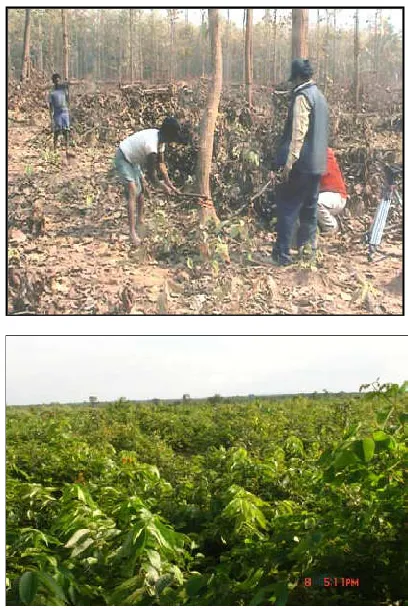
[image:4.612.113.507.257.681.2]

(5)

of surface waterbody (Table 3). By 1999 – 2005, there was decreased in trend of bare surface area, while in 2005 – 2009, there was an increased in trend. Between 1999 and 2009, the low density vegetation zone portrayed increased in trend (i.e., 1114.40 km2), it may be due to the development of settlement and agricultural land and as a result of reclamation process. From 2005 to 2009, the amend of low density and medium density vegetation zone was noteworthy. In the study area, low, medium and high density vegetation showed decreased in trend in the study area. However, some specious results were found in Table 3 and Figure 3b, such as surface waterbody and bare surface areas were increased in 2009. It may be due to fact that the ephemeral streams or irrigation/drainage canals are frequently dry/fill, especially in the monsoonal climate due to heavy rainfall and/or dry environmental conditions. Several erroneous patterns were also obtained in the 2009 results, explicitly, reduce in vegetated land. However, it may be due to anti-social activity and low economic condition in the study area played an important role to diminish the moderate to high density vegetation for their livelihood and to strengthen their economy. In reality, some portion of the study areas (Salboni, Lalgrah, Binpur etc.), vegetated land increased and non-vegetated land decreased (Figure 4).

Accuracy assessment results

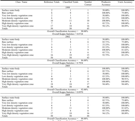
To validate the accuracy of classification procedures of vegetation characteristics accuracy assessment analysis was performed. Tables 4

[image:5.612.80.527.72.473.2]

identify the error matrices resulted from NDVI analysis on different dates. In Table 4, the overall classification accuracy and Kappa statistics were 90.0% and 0.8724, respectively, in 1999. By 2002, the overall accuracy and Kappa statistics of NDVI classes became 86.0% and 0.7934, respectively. Accordingly, the overall classification accuracy and Kappa statistic increased to 92.0%, and 0.8974, respectively in 2009. In 2009, the impressive change among the NDVI classes made due to anthropogenic intervention, and resulting in an

Figure 3b. Surface covered by different group of vegetation at different period (1999-2009) in the study area

Table 4. Error matrices for continuous images for NDVI on different dates in Kangswati (Cossi) river and Dwarakeswar river interfluves area

Class Name Reference Totals Classified Totals Number Correct

Producers Accuracy

Users Accuracy

1999

Surface water body 2 1 1 50.00% 100.00%

Bare surface 6 8 6 100.00% 75.00%

Very low density vegetation zone 2 1 1 50.00% 100.00%

Low density vegetation zone 6 5 5 83.33% 100.00%

Moderate density vegetation zone 10 11 10 100.00% 90.91%

High density vegetation zone 7 6 6 85.71% 100.00%

Very High density vegetation zone 17 18 16 94.12% 88.89%

Totals 50 50 45

Overall Classification Accuracy = 90.00% Overall Kappa Statistics = 0.8724

2002

Bare surface 7 8 6 85.71% 75.00%

Totals 50 50 43

2005

Bare surface 7 8 6 85.71% 75.00%

Totals 50 50 46

2009

Bare surface 7 8 6 85.71% 75.00%

Totals 50 50 44

[image:5.612.317.550.581.712.2]

(6)

[image:6.612.77.281.48.353.2]

Figure 4. Vegetation destruction due to human intervention

overall classification accuracy and Kappa statistics decreased to 88.0% and 0.8472, respectively. The temporal variation of vegetation coverage divulges the time period that key development and alters cropped up. During the last 11 years (1999 – 2009), a remarkable amend of vegetation vigor was observed in the Kangswati and Dwarakeswar river interfluves area. In this research, NDVI analyses were exercised to examine the characteristics of vegetation coverage during this period. According to the research results, the NDVI technique presented more consistent and precise information to scrutinize the modification of vegetation vigor in this area, except during 2009. High commission errors within the vegetation increase class may be apparent due to inter annual dissimilarity in precipitation between 2005 and 2009. However, the procedures botched to accurately differentiate fallow and newly cultivated fields from barren land during this period. The mixed classes with medium resolution Landsat Imagery necessitate information about the actual ground cover types to attain acceptable results.

Acknowledgement

We thank to USGS Earth Explorer Community for freely providing satellite data. We also thank to Geography and Environment Management Department of Vidyasagar University, Midnapur, West Bengal for providing Laboratory facility for Satellite data analysis.

REFERENCES

Bakr N, Weindorf DC, Bahnassy MH, Marei SM, El-Badawi MM 2010. Monitoring land cover changes in a newly reclaimed area

of Egypt using multi-temporal Landsat data. Applied

Geography, 30 (2010) 592–605.

Banner, A., and Lynham, T., 1981, Multitemporal analysis of Landsat data for forest cutover mapping—a trial of two procedures. Proceedings of the 7th Canadian Symposium on Remote Sensing, Winnipeg, Canada, pp. 233–240.

Carmel Y, Kadmon R, Nirel R 2001. Spatiotemporal predictive

models of mediterranean vegetation dynamics. Ecological

Applications, 11(1), 268–280.

Congalton RG 1991. A review of assessing the accuracy of

classifications of remotely sensed data. Remote Sensing of

Environment, 37(1), 35–46.

Congalton RG, Green K (1999). Assessing the accuracy of remotely sensed data: Principles and practices. Boca Raton: Lewis Publishers.

Coppin, P. R., and Bauer, M. E. 1996. Digital change detection in

forest ecosystems with remote sensing imagery. Remote Sensing

Reviews, 13, 207– 234.

Drissi R, Goutouly JP, Forget D, Gaudillere JP, 2009. Nondestructive Measurement of Grapevine Leaf Area by Ground Normalized

Difference Vegetation Index. Agronomy Journal, 101(1): 226 –

231.

Fung, T. 1990. An assessment of TM imagery for land-cover change

detection. IEEE Transactions in Geoscience and Remote

Sensing, 28 (4), 681– 684.

Goslee SC 2011. Analyzing Remote Sensing Data in R: The landsat

Package. Journal of Statistical Software, 43(4): 1-25.

Joshi, PC, 2011. Performance evaluation of vegetation indices using

remotely sensed data. International Journal of Geomatics and

Geosciences, 2(1): 231-240

Justice, C.O., J.R. Townsend, B.N. Holben, C.J. Tucker, 1985. Analysis of the phenology of global vegetation using

meteorological satellite data. International Journal of Remote

Sensing 6(8): 1319-1334

Kogan, F.N. 1990. Remote Sensing of weather impacts on vegetation

in nonhonogeneous areas. International Journal of Remote

Sensing, 11, 1405-1419.

Mas, J. F. 1999. Monitoring land-cover changes: a comparison of

change detection techniques. International Journal of Remote

Sensing, 20 (1), 139– 152.

Neldner, V.J., Wilson, B.A., Thompson, E.J. and Dillewaard, H.A. 2012. Methodology for Survey and Mapping of Regional Ecosystems and Vegetation Communities in Queensland. Version 3.2. Updated August 2012. Queensland Herbarium,

Queensland Department of Science, Information Technology,

Innovation and the Arts, Brisbane. pp.124

Nemani, R., and Running, S. W. 1996. Global vegetation cover

changes from coarse resolution satellite data. Journal of

Geophysical Research, 101, 7157– 7162.

Pen˜ uelas J, Prieto P, Beier C, Cesaraccio C, de Angelis P, de Dato G, Emmett BA, Estiarte M, Garadnai J, Gorissen A, Lang EK, Kroel-Dulay G, Llorens L, Pellizzaro G, Riis-Nielsen T, Schmidt IK, Sirca C, Sowerby A, Spano D, Tietema A. 2007. Response of plant species richness and primary productivity in shrublands along a northsouth gradient in Europe to seven years of experimental warming and drought: reductions in primary

productivity in the heat and drought year of 2003. Global

Change Biology 13: 2563–2581.

Qi J, Marsett RC, Moran MS, Goodrich DC, Heilman P, Kerr YH, Dedieu G, Chehbouni A, Zhang XX 2000. Spatial and temporal dynamics of vegetation in the San Pedro River basin area. Agricultural and Forest Meteorology. 105, 55–68.

Radeloff, V. C., Mladenoff, D. J., and Boyce, M. S. 2000. Effects of interacting disturbances on landscape patterns: budworm

defoliation and salvage logging. Ecological Applications, 10 (1),

233– 247.

Rahman S, Hasan SMR, Islam MA, Maitra MK. Temporal change detection of vegetation coverage of Dhaka using Remote

Sensing. International Journal of Geomatics and Geosciences,

2(2): 481-490, 2011.

Root TL, Price JT, Hall KR, Schneider SH, Rosenzweig C, Pounds JA. 2003. Fingerprints of global warming on wild animals and

plants. Nature, 421: 57–60.

Rouse, J. W., Haas, R. H., Schell, J. A., Deering, D. W., and Harlan, J.C. (1974). Monitoring the vernal advancements and

(7)

retrogradation (greenwave effect) of nature vegetation. NASA/GSFC Final Report. Greenbelt, MD: NASA.

Roy PS, Ravan SA 1996. Biomass estimation using satellite remote sensing data—An investigation on possible approaches for natural forest. J. Biosci., 21(4): 535-561.

Serneels S, Said M, Lambin EF, 2001, Land-cover changes around a major East African wildlife reserve: the Mara ecosystem.

International Journal of Remote Sensing, 22, 3397–3420. Singh RP, Roy S, Kogan F 2003. Vegetation and temperature

condition indices from NOAA AVHRR data for drought monitoring over India. Int. J. Remote Sensing, 24(22): 4393 – 4402.

Tucker, C. J. (1979). Red and photographic infrared linear

combinations for monitoring vegetation. Remote Sensing of

Environment, 8(2), 127–150.

Yin H, Udelhoven T, Fensholt R, Pflugmacher D, Hostert P. How Normalized Difference Vegetation Index (NDVI) Trendsfrom Advanced Very High Resolution Radiometer (AVHRR) and Système Probatoire d’Observation de la Terre VEGETATION (SPOT VGT) Time Series Differ in Agricultural Areas: An

Inner Mongolian Case Study. Remote Sensing. 2012;

4(11):3364-3389.