On Trivial Solution and High Correlation Problems in Deep Supervised Hashing

On Trivial Solution and High Correlation Problems in Deep Supervised Hashing

Yuchen Guo

, Xin Zhao

, Guiguang Ding

, Jungong Han

†_{School of Software, Tsinghua University, Beijing 100084, China}

‡_{School of Computing and Communications, Lancaster University, Lancaster, LA1 4YW, UK}

{yuchen.w.guo,zhaoxin19,jungonghan77}@gmail.com, [email protected]

Abstract

Deep supervised hashing (DSH), which combines binary learning and convolutional neural network, has attracted con-siderable research interests and achieved promising perfor-mance for highly efficient image retrieval. In this paper, we show that the widely used loss functions, pair-wise loss and triplet loss, suffer from the trivial solution problem and usu-ally lead to highly correlated bits in practice, limiting the per-formance of DSH. One important reason is that it is difficult to incorporate proper constraints into the loss functions under the mini-batch based optimization algorithm. To tackle these problems, we propose to adopt ensemble learning strategy for deep model training. We found out that this simple strategy is capable of effectively decorrelating different bits, making the hashcodes more informative. Moreover, it is very easy to par-allelize the training and support incremental model learning, which are very useful for real-world applications but usually ignored by existing DSH approaches. Experiments on bench-marks demonstrate the proposed ensemble based DSH can improve the performance of DSH approaches significant.

Introduction

The number of images on the Internet has been growing rapidly in recent years, necessitating highly efficient index-ing techniques to facilitate large-scale image retrieval. The recent works have demonstrated that hashing is a powerful technique for efficient and accurate image retrieval (Wang et al. 2016). In particular, hashing transforms real-valued image representations into binary hashcodes. Then, based on the extremely fast basic CPU operations, like bit XOR, the hamming distance between hashcodes can be obtained with little time cost. In this way, linearly scanning the the database is fast and the memory cost for storing the database is low. Suppose we have1 billion images and each image is represented as a128-bit binary sequence. It requires just

16GB memory to load all images’ hashcodes and comput-ing the hammcomput-ing distance between a query image and al-l database images takes onal-ly a few seconds (Wang et aal-l. 2015). Because of its outstanding efficiency and accuracy,

∗

This research was supported by the National Natural Science Foundation of China (Grant No. 61571269) and the Royal Society Newton Mobility Grant (IE150997). Yuchen Guo and Xin Zhao contributed equally. Corresponding author: Jungong Han.

Copyright c2018, Association for the Advancement of Artificial

Intelligence (www.aaai.org). All rights reserved.

0.0 0.2 0.4 0.6 0.8 1.0

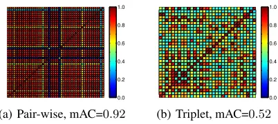
(a) Pair-wise, mAC=0.92

0.0 0.2 0.4 0.6 0.8 1.0

(b) Triplet, mAC=0.52

Figure 1: The correlation matrix (absolute value) of hash-code bits. Different hashhash-code bits are highly correlated.

hashing has been applied to many computer vision tasks, in-cluding not only image retrieval, but also large-scale cluster-ing (Gong et al. 2015), classification (Mu et al. 2014), and re-identification (Zheng and Shao 2016).

Inspired by the great success of convolutional neural networks (CNN) for many computer vision tasks (He et al. 2016), the researchers have made attempt to combine CNN with hashing (Lai et al. 2015; Liong et al. 2015; Liu et al. 2016; Xia et al. 2014). In particular, by slightly modifying the network structure of CNN, especially the out-put layer, we can train a CNN model using the similarity su-pervision as a very effective hashing model which takes the raw image as input and outputs the hashcodes for this im-age. Based on the power of CNN, the deep supervised hash-ing (DSH) model can effectively exploit the semantic simi-larity structure of images and produce better hashcodes than non-deep hashing approaches. For example, Xia et al. (2014) has shown that a simple and straightforward DSH model can improve the mean Average Precision (mAP) over the state-of-the-art non deep approaches by15%(from about35%to about50%) on CIFAR10 (Krizhevsky 2009). With elaborate designs, the mAP achieves60%and more (Liu et al. 2016).

Problem Statement

Howev-er, significantly increasing the hashcode length (say, to128

bits) can only lead to marginal performance gain while many non-deep hashing approaches can be improved a lot, which violates the intuition that longer hashcodes can encode more information such that the intrinsical similarity structure can be better preserved. In practice, we sometimes need longer hashcodes in order to improve the retrieval accuracy if larg-er memory or fastlarg-er computing devices are available. But it seems to be difficult to obtain a better model by simply appending more output units in existing DSH approaches.

To make DSH more practical, it is worth investigating this phenomenon while previous works paid little attention to it. In this paper, we argue that the widely used loss functions in DSH learning, pair-wise loss and triplet loss, are prone to achieving trivial solution, which consequently leads to high-ly correlated bits. Obvioushigh-ly, we cannot expect good perfor-mance using highly correlated hashcodes. For example, if all bits are totally (positively or negatively) correlated, the128 -bit hashcodes will perform just like the1-bit hashcodes. This problem gets more serious for longer hashcodes. To demon-strate it, we first train a DSH model using pair-wise loss (Liu et al. 2016) or triplet loss (Lai et al. 2015). Then the hash-codes for images are extracted. Now we can compute the correlation between different bits. The correlation matrices for different loss functions are shown in Figure 1. We also compute the mean Absolute Correlation for the hashcodes:

mAC= 2

Pk

i=1

P

j>i|Cij|

k(k−1) (1)

wherekis the length of hashcodes andCij is the

correla-tion coefficient between bitiandj. Obviously mAC∈[0,1]

and a larger mAC indicates that the hashcodes have higher correlation. From the figure we can evidently observe that hashcodes are highly correlated even with48bits, and the mAC values also validate the same point. Clearly, it is hard to encode more information by using the highly correlated hashcodes as presented here. In this circumstance, it seem-s reaseem-sonable that exiseem-sting DSH approacheseem-s fail to achieve much better results by simply increasing hashcode length.

Our Contributions

The problems are clear but the solution is not that trivial. In non-deep hashing approaches, some extra constraints and regularizations can be incorporated into the learning objec-tive such that the learned hashcodes are less correlated, like the orthogonality constraint and regularization. However, it is not straightforward to apply these constraints and regu-larizations to DSH because the mini-batch based optimiza-tion algorithm is adopted for deep model training and the model is not aware of the hashcodes of samples out of the mini batch. In this paper, we propose a simple yet effective learning strategy based on ensemble learning which learn-s different bitlearn-s ulearn-sing different training learn-setlearn-s and modellearn-s. We found out that this simple strategy is capable of effectively decorrelating different bits such that the learned hashcodes are more informative, especially for long hashcodes. In this way, given longer hashcodes, more information about the data can be encoded such that more performance

improve-ment can be achieved. Theoretically, we make the following contributions in this paper:

1. We show that the loss functions adopted by existing DSH approaches, pair-wise loss and triplet loss, are prone to trivial solution and produce highly correlated and redundan-t hashcodes. In redundan-this circumsredundan-tance, increasing redundan-the hashcode length can only marginally improve the retrieval accuracy.

2. We propose a simple yet effective ensemble learning based strategy which decorrelates bits and reduces redun-dancy such that longer hashcodes can encode more informa-tion, leading to better performance. To our knowledge, this is the first work noticing the trivial solution and high corre-lation problems in DSH and systematically solve them.

3. Our approach supports incremental learning while ex-isting DSH approaches fail to do so. In particular, when new labeled samples are given, or when longer bits are required, e.g., we change the hashcode length from48to64because better devices are given, existing DSH approaches have to totally retrain a new hashing model for 64-bit hashcodes with all training data. On the contrary, our approach only needs to learn hashing functions for the extra16bits.

4. It is straightforward to parallelize the training which makes the deep model training more efficient and cheap.

Related Work

By representing images as binary codes and taking advan-tage of fast bit operations, hashing can reduce the memo-ry cost and accelerate the search speed with orders of mag-nitudes. Earlier works mostly focused on data-independent hashing, like Locality Sensitive Hashing (Gionis, Indyk, and Motwani 1999) which adopts random splits to bina-rize image features. Because no prior about the data is taken into account, the data-independent approaches usu-ally requires very long hashcodes for satisfactory perfor-mance (Zhang et al. 2010). To design more effective hash-codes, the researchers turned their focus to data-dependent hashing which utilizes the data distribution information. Some widely used priors include the variance of data (Gong et al. 2013; Xu et al. 2013), manifold structure (Guo et al. 2017b; Liu et al. 2014; 2011), the cluster structure (He, Wen, and Sun 2013), and etc. For image retrieval, the user-s care more about the user-semantic user-similarity between imageuser-s. Therefore, many supervised hashing approaches are pro-posed that use the semantic similarity (like the similarity matrix) as supervision to guide the hashing function learn-ing (Ge, He, and Sun 2014; Liu et al. 2012; Shen et al. 2015; Zhang et al. 2014). Because the supervised knowledge is available, the supervised ones yield better retrieval perfor-mance, especially evaluated from the semantic perspective.

CN-Training data

……

0 1 1 0 1 0 0 1

Convolution and

pooling layers fc layers Hashing

layer

Loss Computation

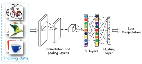
Figure 2: The basic architecture of DSH.

N with the supervised information, deep supervised hash-ing (DSH) achieves promishash-ing retrieval accuracy. Xia et al. (2014) propose a simple CNN based hashing approach that has a disjoint learning procedure and only employs CN-N as a mapping model. Despite its simplicity, it outperform-s outperform-state-of-the-art non-deep haoutperform-shing approacheoutperform-s with outperform- signif-icant margin. To make better use of the power of CNN, Lai et al. (2015) propose an end-to-end architecture that si-multaneously learns the feature mapping functions and the binary codes which minimize the triplet loss. The results demonstrate that the end-to-end learning is better than dis-joint learning. Liu et al. (2016) propose to consider the pair-wise loss and the quantization loss during model learning. Zhang et al. (2015) adopt the similarity regularized triplet loss and achieve state-of-the-art performance for image re-trieval. Generally, the DSH approaches have dominated the leaderboard of hashing based image retrieval in recent years. Please refer to (Wang et al. 2016) for more elaborate survey.

The Proposed Model

Trivial Solution and High Correlation

To clarify the problems, we firstly briefly introduce the basic architecture of DSH, which is illustrated in Fig-ure 2. Typically, there are three components in the net-work modified from some well-established architectures, like AlexNet (Krizhevsky, Sutskever, and Hinton 2012) and VGG (Szegedy et al. 2015). The first component contain-s the convolutional and pooling layercontain-s which adopt nonlin-ear transformation to extract basic image features. The sec-ond component consists of fully connected layers and hash-ing/quantization layers which produce (approximate) binary codes for images. The last component is the loss computa-tion which computes the loss using the hashcodes and the supervised information. Specifically, the supervised knowl-edge is given as the semantic similarity matrix S where sij = +1or−1indicating imagesIi andIj are similar or

not. The objective of DSH learning is to make similar im-ages have similar hashcodes (small hamming distance) and dissimilar images have dissimilar hashcodes (large hamming distance). A simple loss function is pair-wise loss (Li, Wang, and Kang 2016; Liong et al. 2015; Liu et al. 2016) direct translating this objective as below:

Jp₌X

i,jsijd(hi,hj) (2)

wherehi,hj ∈ {−1,1}k are the hashcodes of training

im-age Ii andIj andk is the length of hashcodes (the

num-ber of output units in the hashing network).d(·,·)denotes a distance measure between hashcodes, such as squared Eu-clidean distanced(hi,hj) = khi−hjk22 in (Liong et al.

2015; Liu et al. 2016). In addition, noticing that the retrieval cares more about the ranking than the absolute distance, ranking based loss functions are often used. The most pop-ular one is triplet loss (Lai et al. 2015; Zhang et al. 2015) which considers the relationship of a positive sample and a negative sample to a target sample, which is defined as:

Jt₌X

i,p,nd(hi,h p

i)−d(hi,hni) (3)

wherep andn denote a positive sample (sip = 1) and a

negative sample (sin=−1) to target imageIirespectively. Trivial solution. Looking back to the network architec-ture introduced above, we can notice an important property about the hashcodes. After the final fc layer, the models to generate each hashcode bit are independent to each other. In fact, the last fc layer and the hashing layer are also fully connected. Suppose the output of the last fc layer isgi, the

l-th bit is generated ashil =Q(givl0), whereQis a

quanti-zation function likesignfunction, andvlare the connection

weights between thel-th hashing layer unit and all units of the last fc layer. Forl1 6= l2, becausevl1 andvl2 are free

from each other, they can have totally different or identi-cal values. It is not a critiidenti-cal issue for some other tasks like classification because minimizing the loss functions will as-sign proper values to them. However, for pair-wise loss and triplet loss, the network favors to assign identical values to them. The reason is not that clear, which is discussed below. Firstly, we can see the loss functions in Eq. (2) and Eq. (3) are bit-wise decoupled such that they can be divided intok sub-problems. For example, the pair-wise loss with squared Euclidean distance (Liu et al. 2016) can be rewritten as:

Jp₌X

i,j

sijkhi−hjk22=

X

i,j

X

l

sij(hil−hjl)2

=X

l

X

i,j

sij(hil−hjl)2=

X

l J_lp

(4)

whereJ_lp = P

i,jsij(hil−hjl)

2_{is thel-th sub-loss.}

Af-ter training the DSH network by minimizing the lossJp_,

we obtain the parameters vl and the sub-loss Jlp can

al-so be computed. Now let lm = argminlJ p

l. If we assign

the parametersvlm to all other bits while fixing the

previ-ous layers, we can obtain a new network. Obviprevi-ously, for this network, we haveJp

new=kJ p lm ≤

P

lJ p l =J

p

old. Clearly, Jp

new = J p

old if and only ifJ p l = J

p

lm(∀l = 1, ..., k). In

this circumstance , if we have the optimal solution for one bit, copying its solution to other bits leads to the global opti-mum, which indicates the multi-bit model training problem can be solved trivially by simply learning one bit and then directly assigning its solution to all other bits. In practice, it is an undesired and bad property for multi-bit hashcodes.

The triplet loss has the same problem as the pair-wise loss. In fact, Eq. (3) can also be rewritten in the same way:

Jt₌X

l

X

i,p,n

(hil−hpl)2−(hil−hnl)2=

X

l Jt

Data group 1

……

0 1 1 0

Shared layers

Layer group 1

Data group 2

Data group m

... D

D

Daaattttaaaa ggggrrr u

D D

Daaaattttttttaa gggggrrrorrorrrrrouououuuuuuuupppppppp 22222222222

D

Daaattttaaaa ggggrrrrroooouuu

D D

Daaatattttttaa ggrggggrrrrrrroo

1 1 0 0

Layer group 2 ...

1 0 1 0

Layer group m

Loss Loss

Loss

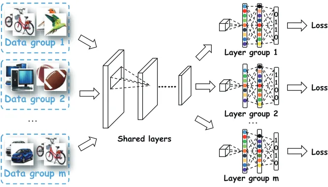
Figure 3: Ensemble based DSH. Several training subsets are sampled from the original training set (different data). Each subset is used to train a DSH sub-model producing _mk-bit hashcode(different models). To speed up the training and code generation, we freeze the first few layers and share them among all sub-models. Each sub-model only needs to optimize its specific part.

Like the case of pair-wise loss, triplet loss also suffers from trivial solution problem due to its bit-wise decoupled loss.

In non-deep hashing, it is easy to incorporate proper con-straints or regularizations into the loss function, such as the orthogonality constraintH0H = nIk or regularization kH0H−nIkk2Fon all bits to avoid the trivial solution.

How-ever, in DSH, the mini-batch based optimization algorithm is adopted such that the network can see only a small batch of data. In this way, it cannot compute the orthogonality loss which needs all data to compute or backpropagate it.

High correlation.Eq. (2) and Eq. (3) are the simplest loss functions. In practice, several works attempt to perform a further nonlinear transformation on the distance. For ex-ample, a distance margin can be incorporated. For pair-wise loss, Liuet al.(Liu et al. 2016) reformulate Eq.(2) as below:

Jp₌ X

sij=1

d(hi,hj) +

X

sij=−1

max(0, λ−d(hi,hj)) (6)

whereλ ≤ k is the margin parameter. The triplet loss can also be reformulated using the margin (Lai et al. 2015):

Jt₌ X

i,p,n

max(0, λ+d(hi,hpi)−d(hi,hni)) (7)

The nonlinear transformation can theoretically prevent the learning from trivial solution. However, the model usually achieve a near trivial solution at last, which appears to have highly correlated hashcodes. As shown in Figure 1, the mAC of 32-bit hashcodes is 0.52 with the margin based triplet loss (Lai et al. 2015), and it gets larger for longer codes.

Ensemble based DSH

To address this issue, we propose an ensemble based strategy for DSH learning. Inspired by the classifier ensemble (Diet-terich 2000), we can consider three different ways to decor-relate bits. The first is random initialization. Although the

global optimum for each bit should be identical, the deep model adopts gradient descent for optimization such that different initializations are likely to result in different lo-cal optimum, which reduces the correlation between bits. In fact, the existing DSH approaches benefit from the ran-dom initialization and they perform well with short hash-codes. However, when the hashcodes are too long (say,128

bits), the random initialization does not work well, leading to high correlation. The second is to use different training data. This is widely used for classifier ensemble, including many boosting algorithms. It is very easy to construct differ-ent sub training sets for hashing model learning as hashing is designed for large-scale problem such that there are always sufficient training data. The third is to utilize different mod-els. In DSH, we can achieve this goal by simply changing the network architecture, like the number of fc layer units.

Based on the above discussion, we consider to use differ-ent training data and models, as illustrated in Figure 3. Giv-en a training set, we randomly samplemgroups where each group is utilized to train one model. As there aremgroups, each model only needs to output _mk bits. For example, if our target is128-bit hashcode, we can trainm= 8sub-models and each sub-model outputs16bits. Then we can concate-nate the 16-bit sub-hashcode produced by each sub-model to obtain the final128-bit hashcode for an image.

should be task independent. In this way, all sub-models can share these layers to reduce computational cost. Only the last few layers, such as the fc layers and the hashing layer which are more related to the specific tasks, need further tuning by its corresponding data group. It is also simple to change the architecture of these layers. For example, we can reduce the number of hidden units in a fc layer by half, or the number of filters in the last convolutional layer by half, which can respectively lead to different models. Obviously, the models with different network architectures have different optimum such that their hashcodes have less inter-group correlation.

Parallelization and Incremental Learning

Parallelization. We can notice that training the t-th sub-model using thet-th data group has no influence on the other m−1groups. So we can parallelize the model training and train each sub-model independently. As a sub-model only has _mk output units, which are far fewer than that of one u-nified model as in existing approaches, and the training set is also relatively smaller because we only sample a subset from the training data, the training can converge faster. In this way, the training procedure is somehow accelerated.

Incremental Learning.Incremental learning is very im-portant in practice. For example, when some new training samples are given, we can use it to update the hashing model. However, existing DSH approaches have to use all training data, including previous data and new data, to re-train the whole model. If only new data is utilized, the model may “forget” the previous knowledge. In the ensemble learning, we can use the new samples as a data group and only up-date one sub-model. In this way, the abundant knowledge from previous training data can be maintained by the other sub-models, and the new knowledge can be included by the updated sub-model. In addition, if better computing devices are available such that we can increase the hashcode length for more accurate retrieval. Existing DSH approaches have to re-train all bits from scratch while the proposed ensemble based DSH only needs to train more sub-models and reuse the previous ones. In this way, the previous knowledge and sub-models can be fully reused to save the training expense.

Experiment

Datasets and Settings

CIFAR10(Krizhevsky 2009). CIFAR10 has10kinds of ob-jects such as “bird”, “ship”, and “frog”. For each category there are6,000images belonging to it. For this dataset, we randomly sample1,000images (100images per category) as the query set, and the remaining59,000images form the database. Moreover, in the database, we further randomly sample10,000images as training set for model learning.

Animals with Attributes (Lampert, Nickisch, and Harmeling 2014). AwA dataset is collected from Web which consists of50animal species. There are30,475images in AwA. We randomly sample 1,000 images (20 images per category) as the query set, and the remaining29,475images as database where10,000images are used for training.

ImageNet(Russakovsky et al. 2015). ImageNet is a well-known benchmark dataset for the Large Scale Visual

Recog-nition Challenge (ILSVRC). It has1,000object categories with about1.2million training images and50thousand val-idation images. Following (Guo et al. 2017a), we randomly select100 categories which leads to a database with about

120thousand images and a query set with about5,000 im-ages. In this dataset,10,000images (100 per category) are randomly selected from the database for training models.

We adopt the widely used mean Average Precision (mAP) as the numeric evaluation metric. We also report the precision-recall curve to compare the retrieval performance. Following the widely used setting in previous works (Guo, Ding, and Han 2017; Liong et al. 2015; Liu et al. 2016; Xia et al. 2014; Zhuang et al. 2016; Zheng, Tang, and Shao 2016; Zheng and Shao 2016), a database image is considered as a true positive of a query image if they share the same label.

Implementation Details

Our ensemble based DSH can be regarded as a general framework such that it can be combined with previous DSH approaches. In the experiment, we basically consider the pair-wise loss (Liu et al. 2016) and the triplet loss (Lai et al. 2015). To construct different data groups for training, we adopt a random complementary sampling strategy. In partic-ular, we randomly sample half of training data (5,000 im-ages in our experiment) for the first data group and then we use the other half for the second group. Next, we again ran-domly sample half of training data for the third group and the other half for the fourth group. We continue the procedure untilmgroups are obtained. In this way, we can guarantee that all data are equally used for training form/2times and each group can be as different from the others as possible.

In the experiment, we utilize theCaffe(Jia et al. 2014) tool and we adopt AlexNet (Krizhevsky, Sutskever, and Hin-ton 2012) pre-trained on ImageNet classification task as the base network which has5convolutional layers (withReLU

layers and pooling layers) and2fully connected layers. We further add another hashing layer at the end of the network to producek-bit hashcodes. In fact, we can surely adopt more complicated network such as ResNet (He et al. 2016). But it is unclear whether the performance gain over the other approaches is given by our method or a powerful network. Hence, we adopt a relatively simple but effective network.

How Many Layers to Share?

As introduced before, the ensemble learning based DSH needs to trainmdifferent sub-models where each produces

k

m bits. If all sub-models are totally different, the training

Table 1: mAP Comparison on benchmark datasets.

ImageNet CIFAR10 AwA

32bits 64bits 96bits 128bits 32bits 64bits 96bits 128bits 32bits 64bits 96bits 128bits

LSH 0.2350 0.3596 0.4172 0.4584 0.2553 0.2940 0.3224 0.3380 0.1870 0.2249 0.2617 0.2889 KSH 0.2976 0.3943 0.4472 0.4851 0.5080 0.5572 0.5666 0.5798 0.3279 0.3751 0.4089 0.4262 SDH 0.2804 0.3897 0.4592 0.5016 0.5140 0.5520 0.5644 0.5879 0.3279 0.3751 0.4089 0.4262 LFH 0.2349 0.3417 0.4105 0.4484 0.2665 0.3519 0.4128 0.4493 0.2420 0.2977 0.3472 0.3689

CNNH 0.4498 0.5038 0.5294 0.5380 0.4720 0.4990 0.5133 0.5370 0.4498 0.4831 0.4942 0.5099 DeSH 0.4651 0.5132 0.5287 0.5472 0.6390 0.6441 0.6473 0.6520 0.5174 0.5300 0.5347 0.5380 DNNH 0.4931 0.5343 0.5431 0.5576 0.6199 0.6317 0.6489 0.6531 0.5285 0.5484 0.5577 0.5607 DRSCH 0.4752 0.5277 0.5301 0.5399 0.6287 0.6326 0.6338 0.6390 0.5010 0.5075 0.5159 0.5190 Ours 0.4946 0.5631 0.5831 0.6156 0.6421 0.6622 0.6989 0.7051 0.5494 0.5804 0.5960 0.6078

0.0 0.2 0.4 0.6 0.8 1.0

(a) 32 bits, mAC= 0.38

0.0 0.2 0.4 0.6 0.8 1.0

(b) 64 bits, mAC= 0.52

0.0 0.2 0.4 0.6 0.8 1.0

(c) 96 bits, mAC= 0.64

0.0 0.2 0.4 0.6 0.8 1.0

(d) 32 bits, mAC= 0.73

0.0 0.2 0.4 0.6 0.8 1.0

(e) 32 bits, mAC= 0.17

0.0 0.2 0.4 0.6 0.8 1.0

(f) 64 bits, mAC= 0.21

0.0 0.2 0.4 0.6 0.8 1.0

(g) 96 bits, mAC= 0.23

0.0 0.2 0.4 0.6 0.8 1.0

(h) 128 bits, mAC= 0.25

Figure 4: The correlation matrix and mAC values of (Lai et al. 2015) (the first row) and ours (the second row).

in Table 2. Generally, we can observe that the results change a little if we only fix the first3layers, which is consistent with our intuition because the first few layers focus on the low-level features, like edges and corners of images. More-over, if some layers likeconv5are fixed, the retrieval per-formance drops significantly because these layers are more task-specific. From the results we can see that fixingconv1

toconv3is a good balance between efficiency and accuracy. In the following experiments, we keepconv1toconv3fixed for each sub-model if no more statement is given.

The Correlation of Hashcodes

The reason why existing DSH approaches fail to achieve sig-nificant gain using longer hashcode is because their hash-codes are highly correlated such that longer hash-codes cannot encode more information. To address this issue, we adopt an ensemble based strategy for DSH. In this part we investigate the ability of ensemble based DSH to decorrelate bits. We use AwA dataset and triplet loss (Lai et al. 2015).

We also use16bits for each sub-model. The correlation matrices and the corresponding mAC values by Eq. (1) are shown in Figure 4. Benefiting from the random initialization and the margin in the loss function, (Lai et al. 2015) can achieve about 0.20mAC with16bits and 0.38mAC with

Table 2: The influence of fixed layers. This table shows the mAP when fixing layers between the first to the target layer.

layers pair-wise triplet layers pair-wise triplet

none 0.5871 0.6022 conv1 0.5852 0.5991 conv2 0.5793 0.5942 conv3 0.5717 0.5831 conv4 0.5434 0.5668 conv5 0.5173 0.5412 fc6 0.4647 0.5082 fc7 0.4190 0.4378

32bits. However, when we increase the hashcode length to

64and more, the correlation increases very fast and reaches

0.73mAC with128bits. On the contrary, with the ensemble based strategy, we can significantly suppress the correlation and the mAC only reaches0.25with128bits, indicating our approach can encode more information in the hashcodes.

Benchmark Comparison

Now we compare our approach against existing hashing ap-proaches on benchmark datasets. Based on the results shown in Table 2, we use triplet loss and freezeconv1 to conv3

0 0.5 1 0

0.3 0.6 0.9

Recall

Precision

Ours DNNH DeSH DRSCH CNNH

(a) ImageNet, 64 bits

0 0.5 1

0 0.3 0.6 0.9

Recall Precision Ours_DNNH

DeSH DRSCH CNNH

(b) CIFAR10, 64 bits

0 0.5 1

0 0.3 0.6 0.9

Recall

Precision

Ours DNNH DeSH DRSCH CNNH

(c) AwA, 64 bits

0 0.5 1

0 0.3 0.6 0.9

Recall

Precision

Ours DNNH DeSH DRSCH CNNH

(d) ImageNet, 128 bits

0 0.5 1

0 0.3 0.6 0.9

Recall Precision Ours

DNNH DeSH DRSCH CNNH

(e) CIFAR10, 128 bits

0 0.5 1

0 0.3 0.6 0.9

Recall Precision Ours

DNNH DeSH DRSCH CNNH

(f) AwA, 128 bits

Figure 5: The precision-recall curves of DSH approaches.

As our approach supports incremental learning, we train our model in an incremental way. For example, we train2 sub-models for 32-bit experiment. Then for 64-bit experimen-t, we reuse these 2 sub-models and only train2 new sub-models. On the other hand, for other approaches, we totally train a new model for each hashcode length.

We select the following hashing approaches as baselines. Locality Sensitive Hashing (LSH) (Gionis, Indyk, and Mot-wani 1999), and three state-of-the-art supervised hashing approaches, Kernelized Supervised Hashing (KSH) (Liu et al. 2012), Supervised Discrete Hashing (SDH) (Shen et al. 2015), and Latent Factor Hashing (LSH) (Zhang et al. 2014). For these non-deep approaches, we use the output of fc7

layer of pre-trained AlexNet as input features. More impor-tantly, we select four state-of-the-art deep supervised hash-ing approaches, CNNH (Xia et al. 2014), DeSH (Liu et al. 2016), DNNH (Lai et al. 2015), and DRSCH (Zhang et al. 2015). For all approaches, including all baselines and ours, we use the same query-database-train split for fairness.

The mAP comparison are summarized in Table 1 and the precision-recall curves of all DSH approaches are shown in Figure 5. Clearly, the deep approaches significantly out-perform non-deep approaches, especially with short hash-code length, like 32 bits, which is consistent with the re-sults in previous literatures (Lai et al. 2015; Liu et al. 2016; Xia et al. 2014; Zhang et al. 2015). However, there is one important observation we need to highlight, which is not fully discussed in previous works, that the DSH approach-es’ performance increases very slowly. From32bits to128

bits, the end-to-end DSH approaches, DeSH, DNNH, and DRSCH increase mAP by3.86%,4.33%, and 3.10% re-spectively in average. The reason is that they obtain highly correlated bits in long hashcodes such that they fail to en-code more information, which has been discussed heavily in

this paper. Our approach is comparable to the baselines with

32bits, which is much better than non-deep approaches. But we can observe that our approach is able to further improve its performance with longer hashcodes. In particular, our ap-proach increases mAP from32bits to128bits by 8.07%, which is far larger than the other DSH approaches. More-over, the average performance gap between our approach and best DSH approach is2.63%,4.28%, and5.24%with

64bits,96bits, and128bits respectively, getting larger with longer codes. Both observations, together with the results in Figure 4, demonstrate that our approach can effectively decorrelate bits and prevent the triplet loss and from triv-ial solution and high correlation problems, making the hash-codes more informative. Moreover, the results also show our approach works well in the incremental learning, which is very useful for real-world applications.

Conclusion

References

Dietterich, T. G. 2000. Ensemble methods in machine learning. In

Multiple Classifier Systems, First International Workshop, 1–15. Ge, T.; He, K.; and Sun, J. 2014. Graph cuts for supervised binary

coding. InECCV.

Gionis, A.; Indyk, P.; and Motwani, R. 1999. Similarity search in

high dimensions via hashing. InVLDB.

Gong, Y.; Lazebnik, S.; Gordo, A.; and Perronnin, F. 2013. Iterative quantization: A procrustean approach to learning binary codes for

large-scale image retrieval.IEEE TPAMI.

Gong, Y.; Pawlowski, M.; Yang, F.; Brandy, L.; Bourdev, L. D.; and Fergus, R. 2015. Web scale photo hash clustering on a single

machine. InCVPR.

Guo, Y.; Ding, G.; Han, J.; and Gao, Y. 2017a. Sitnet: Discrete

similarity transfer network for zero-shot hashing. InIJCAI.

Guo, Y.; Ding, G.; Liu, L.; Han, J.; and Shao, L. 2017b. Learning to

hash with optimized anchor embedding for scalable retrieval.IEEE

TIP.

Guo, Y.; Ding, G.; and Han, J. 2017. Robust quantization for

general similarity search.IEEE TIP.

He, K.; Zhang, X.; Ren, S.; and Sun, J. 2016. Deep residual

learn-ing for image recognition. InCVPR.

He, K.; Wen, F.; and Sun, J. 2013. K-means hashing: An affinity-preserving quantization method for learning binary compact codes.

InCVPR.

Jia, Y.; Shelhamer, E.; Donahue, J.; Karayev, S.; Long, J.; Girshick, R.; Guadarrama, S.; and Darrell, T. 2014. Caffe:

Convolution-al architecture for fast feature embedding. arXiv preprint

arX-iv:1408.5093.

Krizhevsky, A.; Sutskever, I.; and Hinton, G. E. 2012. Imagenet

classification with deep convolutional neural networks. InNIPS.

Krizhevsky, A. 2009. Learning multiple layers of features from

tiny images. InTech Report. University of Toronto.

Lai, H.; Pan, Y.; Liu, Y.; and Yan, S. 2015. Simultaneous feature

learning and hash coding with deep neural networks. InCVPR.

Lampert, C. H.; Nickisch, H.; and Harmeling, S. 2014. Attribute-based classification for zero-shot visual object categorization.

IEEE TPAMI.

Li, W.; Wang, S.; and Kang, W. 2016. Feature learning based deep

supervised hashing with pairwise labels. InIJCAI.

Liong, V. E.; Lu, J.; Wang, G.; Moulin, P.; and Zhou, J. 2015. Deep

hashing for compact binary codes learning. InCVPR.

Liu, W.; Wang, J.; Kumar, S.; and Chang, S. 2011. Hashing with

graphs. InICML.

Liu, W.; Wang, J.; Ji, R.; Jiang, Y.; and Chang, S. 2012. Supervised

hashing with kernels. InCVPR.

Liu, W.; Mu, C.; Kumar, S.; and Chang, S. 2014. Discrete graph

hashing. InNIPS.

Liu, H.; Wang, R.; Shan, S.; and Chen, X. 2016. Deep supervised

hashing for fast image retrieval. InCVPR.

Mu, Y.; Hua, G.; Fan, W.; and Chang, S. 2014. Hash-svm: Scalable

kernel machines for large-scale visual classification. InCVPR.

Russakovsky, O.; Deng, J.; Su, H.; Krause, J.; Satheesh, S.; Ma, S.; Huang, Z.; Karpathy, A.; Khosla, A.; Bernstein, M. S.; Berg, A. C.; and Li, F. 2015. Imagenet large scale visual recognition challenge.

IJCV.

Shen, F.; Shen, C.; Liu, W.; and Shen, H. T. 2015. Supervised

discrete hashing. InCVPR.

Szegedy, C.; Liu, W.; Jia, Y.; Sermanet, P.; Reed, S. E.; Anguelov, D.; Erhan, D.; Vanhoucke, V.; and Rabinovich, A. 2015. Going

deeper with convolutions. InCVPR.

Wang, J.; Wang, J.; Song, J.; Xu, X.; Shen, H. T.; and Li, S. 2015.

Optimized cartesian k-means.IEEE TKDE.

Wang, J.; Zhang, T.; Song, J.; Sebe, N.; and Shen, H. T. 2016. A

survey on learning to hash.CoRRabs/1606.00185.

Xia, R.; Pan, Y.; Lai, H.; Liu, C.; and Yan, S. 2014. Supervised hashing for image retrieval via image representation learning. In

AAAI.

Xu, B.; Bu, J.; Lin, Y.; Chen, C.; He, X.; and Cai, D. 2013.

Har-monious hashing. InIJCAI.

Yosinski, J.; Clune, J.; Nguyen, A. M.; Fuchs, T. J.; and Lipson, H. 2015. Understanding neural networks through deep visualization.

CoRRabs/1506.06579.

Zhang, D.; Wang, J.; Cai, D.; and Lu, J. 2010. Self-taught hashing

for fast similarity search. InSIGIR.

Zhang, P.; Zhang, W.; Li, W.; and Guo, M. 2014. Supervised

hashing with latent factor models. InSIGIR.

Zhang, R.; Lin, L.; Zhang, R.; Zuo, W.; and Zhang, L. 2015. Bit-scalable deep hashing with regularized similarity learning for

im-age retrieval and person re-identification.IEEE TIP.

Zheng, F., and Shao, L. 2016. Learning cross-view binary identities

for fast person re-identification. InIJCAI.

Zheng, F.; Tang, Y.; and Shao, L. 2016. Hetero-manifold

regular-ization for cross-modal hashing.IEEE TPAMI.

Zhuang, B.; Lin, G.; Shen, C.; and Reid, I. 2016. Fast training of