ISSN Online: 2327-7203 ISSN Print: 2327-7211
Evaluating Common Strategies for the
Efficiency of Feature Selection in the
Context of Microarray Analysis
Melania Pintilie1, Jenna Sykes2
1Department of Biostatistics, University Health Network, Toronto, Canada 2Department of Respirology, St. Michael’s Hospital, Toronto, Canada
Abstract
The recent explosion of high-throughput technology has been accompanied by a corresponding rapid increase in the number of new statistical methods for developing prognostic and predictive signatures. Three commonly used feature selection techniques for time-to-event data: single gene testing (SGT), Elastic net and the Maximizing R Square Algorithm (MARSA) are evaluated on simulated datasets that vary in the sample size, the number of features and the correlation between features. The results of each method are summarized by reporting the sensitivity and the Area Under the Receiver Operating Cha-racteristic Curve (AUC). The performance of each of these algorithms de-pends heavily on the sample size while the number of features entered in the analysis has a much more modest impact. The coefficients estimated utilizing SGT are biased towards the null when the genes are uncorrelated and away from the null when the genes are correlated. The Elastic Net algorithms per-form better than MARSA and almost as well as the SGT when the features are correlated and about the same as MARSA when the features are uncorrelated.
Keywords
Elastic Net, MARSA, LASSO, Feature Selection
1. Introduction
Discovering prognostic or predictive signatures is a worthwhile endeavor as it is well known that the effect of a treatment is largely heterogeneous. The medical research has witnessed a recent explosion of high-throughput technology, ren-dering the measurement of a large number of genetic features possible. Corres-pondingly, new analytical techniques are constantly being developed to process How to cite this paper: Pintilie, M. and
Sykes, J. (2017) Evaluating Common Strat-egies for the Efficiency of Feature Selection in the Context of Microarray Analysis. Journal of Data Analysis and Information Processing, 5, 11-32.
https://doi.org/10.4236/jdaip.2017.51002
Received: October 6, 2016 Accepted: February 6, 2017 Published: February 9, 2017
Copyright © 2017 by authors and Scientific Research Publishing Inc. This work is licensed under the Creative Commons Attribution International License (CC BY 4.0).
and draw associations from this daunting amount of information. However, the rapid development of both aspects—the measurement and analysis of features— has made it difficult to determine the best analytical technique for finding a ge-netic signature.
To find a genetic signature, an algorithm is applied which ultimately com-bines several features into a single risk score, associated with the outcome [1] [2] [3] [4] [5]. The strength of the association between the risk score and the out-come depends heavily on the features which defines it. If the selected genes have little or no value in explaining the outcome, it is unlikely that a signature created using their values would be useful. Thus, the selection process is of paramount importance in the process of defining a signature. The selected features are typi-cally studied in the laboratory (in vitro and in vivo). Thus, a well-chosen subset of features is contributing to a rapid development of new treatment strategies.
In this paper, we present several algorithms for feature selection for a time-to- event outcome. By using simulated data, we know which features are associated with patient outcome and therefore are able to assess the performance of a tech-nique by calculating the sensitivity and the Area Under the Receiver Operating Characteristic Curve (AUC). Throughout the paper, we use the term “gene” to represent the feature of a high-throughput analysis, which can be a probe set, clone, gene expression or any other molecular feature measured in a continuous manner. The primary aim of this paper is to evaluate the performance of the se-lection process and not the performance of the signature itself.
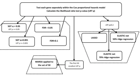
Three algorithms are chosen for evaluation (Figure 1): single gene testing (SGT), Least Absolute Shrinkage and Selection Operator (LASSO) [6] and its extension, the Elastic Net [7] and the Maximizing R Square Algorithm (MARSA, [5]). Each algorithm is applied to the same simulated data in which a number of genes are known to be associated with patient survival.
These algorithms were chosen because they are commonly used in the litera-ture [8] and they are considered substantially different from each other. SGT is used extensively by itself or in combination with other strategies. LASSO and Elastic Net are well-defined statistical algorithms which have been recently gaining in popularity. MARSA is an in-house strategy developed at the Princess Margaret Cancer Centre. This strategy was used to find a signature which could separate patients with low vs. high risk of dying from non-small lung cancer [9]. The signature found using this strategy was validated in 5 independent datasets [9].
Figure 1. The diagram of the algorithms used.
750 which is a reasonable number of genes to start any of the latter selection al-gorithms.
To our knowledge, the MARSA technique has not been properly evaluated until now and this paper is the first to compare feature selection algorithms for time-to-event outcomes using completely simulated datasets with varying sam-ple sizes, with both positive and negative association with outcome and different levels of correlations between predictors.
the association between the predictors and the outcome and the strength of cor-relation between predictors. Their conclusion was that in general, LASSO was preferable, but the differences between the algorithms were small.
In the next section, we present the theoretical formulation for each of these algorithms. The details on simulations can be found in Section 3 and the results in Section 4. In Section 5, we summarize the results and provide conclusions.
2. Description of the Three Strategies
2.1. Single Gene Testing (SGT)
Single gene testing (SGT) is a simple algorithm in which each gene is tested for its association with patient survival separately using the most common tech-nique for survival analysis: the Cox proportional hazards (PH) model [12]. In this approach, the hazard for developing the outcome is assumed to have the form:
( )
| 0( )
i x i
h t x =h t eβ (1)
where h0(t) refers to the baseline hazard, xi is the value for the gene expression for a specific patient i and β is the coefficient obtained by maximizing the partial likelihood:
( )
1 ij i x n x i j R e L e β β β = ∈ =
∏
∑
(2)with Ri being the risk set at time ti. In this paper, all genes with a Likelihood Ra-tio Test (LRT) p-value of less than a particular value α (0.05 and 0.001 [13]) are considered significant and henceforth retained as part of the signature. A stricter α level would have a higher rate of false negative genes while a more relaxed al-pha will have a higher rate of false positives. Alternatively, the genes are also se-lected based on the False Discovery Rate (FDR) [14] using a FDR of 0.05 and 0.1. In this paper, the analysis is performed using the survival package in R but any standard statistical software can be employed.
2.2. Least Absolute Shrinkage and Selection Operator (LASSO) and the Elastic Net
LASSO is a penalized likelihood regression model introduced originally by Tib-shirani (1997). This method has exhibited increased popularity as a feature se-lection technique in the biomedical field with more than 30 articles using this method either alone or in combination with another method [15]-[45]. This method is applied to the Cox PH model with the following restriction imposed on the coefficients:
1
p j
j= β ≤s
∑
(3)this way as a selection process. A larger s will allow fewer non-zero coefficients as compared to a smaller s.
More recently [7], LASSO was extended to incorporate ridge regression using the following restriction:
(
)
( )
21 1 1
p p
j j
j j c
α
∑
= β + −α∑
= β ≤ (4)The parameter α balances how much LASSO restriction is involved in com- parison to ridge-type restriction. When α=1 there is a purely LASSO restriction and when α = 0 there is a ridge-type restriction. When 0 < α < 1, this technique is known as Elastic Net. As α decreases and the ridge restriction component in-creases, more covariates are selected.
In essence, the estimate of the coefficients are found as [46]:
( )
1
2
ˆ arg max log j
i x m
i
i x j Re P
n
β
β α
β=
∑
= β− ∑
∈ −λ β (5)
where
( )
(
)
21 1 1 1 2 p p i i i i Pα
λ β =λ α = β + −α = β
∑
∑
, m is the number of events,nthe number of observations and p the number of covariates. The bold items represent vectors and the xT represents the transpose of vector x.
The parameter λ is chosen such that it maximizes the K-fold cross validation log partial likelihood (CVL) introduced by Verveij and van Houwelingen [47].
( )
( )
(
)
( )(
( )( )
)
{
1,}
ˆ arg max ˆ ˆ
k k k
k K l β λ l β
λ=
∑
= − − − − λ (6)where the subscript (-k) indicates that the k-th subset of the data is left out. LASSO and Elastic Net are recommended when the number of covariates in the model is large, often exceeding the number of observations, and the cova-riates are correlated. To mimic a real life scenario only the genes with a p-value <= 0.2 were considered for this algorithm. By choosing a relaxed α level of 0.2 we want to ensure that all the genes with some potential are included while keeping the false negative rate to a minimum.
The two methods can be performed using the glmnet package in R. The pa-rameter λˆ is based on cross-validation. Since each run of the cross-validation will produce a slightly different value for λ, the cross-validation was repeated 5 times and the median of the 5 resulting values was the one utilized in the subse-quent steps.
2.3. Maximizing R Square Algorithm (MARSA)
2
1.645 S R
S
β β β β
=
+ (7) where β is the coefficient obtained in the CoxPH model and S is the variance of the covariate.
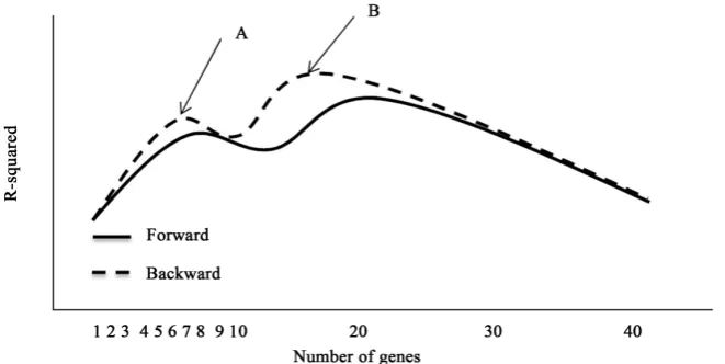
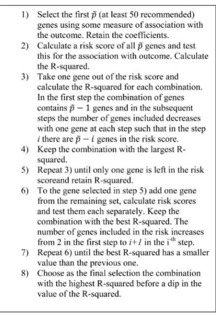
[image:6.595.210.541.523.689.2]The first step is to select a number of candidate genes. To order the genes, we used the LRT p-value when each single gene is tested and selected the first p = 50 genes when 10 genes were associated with outcome (case A) and p = 60 when 20 genes were associated with outcome (case B) and p = 120 when 60 genes were associated with outcome (case C, please Section 3 for the description of the cases A-C). The run-time for the algorithm increases (approximately n2) with the number of genes included. The selection process starts with a risk score based on all genes. In a backward selection fashion, all risk scores which are based on all genes but one (that is, p − 1 genes) are fitted using Cox proportional hazards model and the set with the best R-squared is kept. Next, all the risk scores based on the sets of p − 2 genes obtained from the winner of the p − 1 sets is calcu-lated, tested and the model with the highest R-squared is kept. This process is repeated until the risk score is based on just a single gene. A forward selection is then applied by starting with this one gene and adding each one of the genes not yet in the risk score. At each step the R-squared is retained. In this way, a series of R-squared values are obtained for each number of genes from p to 1 in the backward phase of selection and another series in the forward phase of the selec-tion. The smallest set of genes for which the R-squared value does not drop by adding another gene is selected as the constituent parts of the signature. Figure 2 presents a graphical display of this criterion. Although the highest R-squared is at B with approximately 18 genes in the risk score, our algorithm would choose point A with approximately 6 genes in the risk score. When the R-squared de-creases as the number of genes inde-creases, it is a sign that the R-squared has reached its full potential. The high value at point B is due to overfitting rather than due to a real signal (Figure 3).
Figure 3. The steps for MARSA algorithm.
3. Description of the Simulation
In this paper, the term “correlated genes” refers to the genes which are corre-lated among themselves and “association with survival” refers to the relationship of the genes with patients’ survival. The number of generated genes is realistic as all algorithms, except the SGT based on the p-value, are usually applied on a subset of the genes and not on the whole array.
3.1. Case A (Table 1)
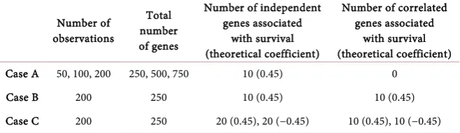
To investigate the performance of the three algorithms described above in rela-tion to the sample size and the number of genes in the dataset, nine datasets were generated from a standard normal distribution with different number of genes (p = 250, 500 and 750) and different number of patients (n = 50, 100 and 200). The genes were simulated to be independent of each other. For each of these sets, survival data were generated such that the first 10 genes were asso-ciated with survival with a coefficient of 0.45. The rest of p-10 genes were not associated with survival.
3.2. Case B (Table 1)
Table 1. Summary of the parameters used for the simulations.
Number of observations
Total number of genes
Number of independent genes associated
with survival (theoretical coefficient)
Number of correlated genes associated
with survival (theoretical coefficient)
Case A 50, 100, 200 250, 500, 750 10 (0.45) 0
Case B 200 250 10 (0.45) 10 (0.45)
Case C 200 250 20 (0.45), 20 (−0.45) 10 (0.45), 10 (−0.45)
Thus, it was considered that 20 genes were associated with survival (coefficient 0.45) and 10 of these were correlated among themselves.
3.3. Case C (Table 1)
For the same situation of p = 250 and n = 200 we considered the situation where 60 genes were associated with survival; 30 positively associated with death (coef-ficient 0.45) and 30 negatively associated with death (coef(coef-ficient −0.45). Ten of the first 30 were correlated among themselves as well as 10 of the second group of 30. The correlation coefficients varied as before (0, 0.4, 0.6, 0.8).
3.4. Generating the Survival Times
The survival times were generated as exponentially distributed with the hazard:
(
)
101 | 0.2 i i ix h t X = e∑=β
with βi the coefficient of the ith covariate. To obtain approximately 50% events in each dataset, the censoring time was generated as uniformly distributed between 2 and 5, representing an accrual time of 3 years and a follow-up time of 2 years. The coefficients (0.45 and −0.45) were chosen such that the power to detect sig-nificance for one covariate with 50, 100 and 200 records varies and reflects real- life situations. For α = 0.001 the power for n = 50, 100 and 200 is 15%, 46% and 89% respectively and for alpha = 0.05 the power is 61%, 89% and 99% respec-tively.
All simulations were performed 2000 times. Each algorithm (SGT, LASSO, Elastic Net (α = 0.3), Elastic Net (α = 0.7), and MARSA) was applied to each of the simulated dataset. Data presented in this paper is based solely on simulation and do not contain any piece of information collected from patients. As such, consent was not necessary.
4. Evaluation of the Simulation
positive and false negative genes. Arguably, of the two types of false results, the false negative may be more damaging since the false positive genes could be weeded out through a second process of validation using a different platform (like Polymerase Chain Reaction (PCR)). On the other hand, the false negative genes are lost completely. Sensitivity is a good measure to assess which scenarios would minimize the false negative genes.
A gene was considered as selected if it was significant and the direction of the detected association corresponded to the theoretical one. A disregard of the di-rection of significance would inappropriately inflate the results. For example if one of these methods has the tendency to select a positive gene but to estimate the effect in the opposed direction then it may appear that it is better than another method which selects fewer genes but with the correct direction.
5. Results of the Simulation
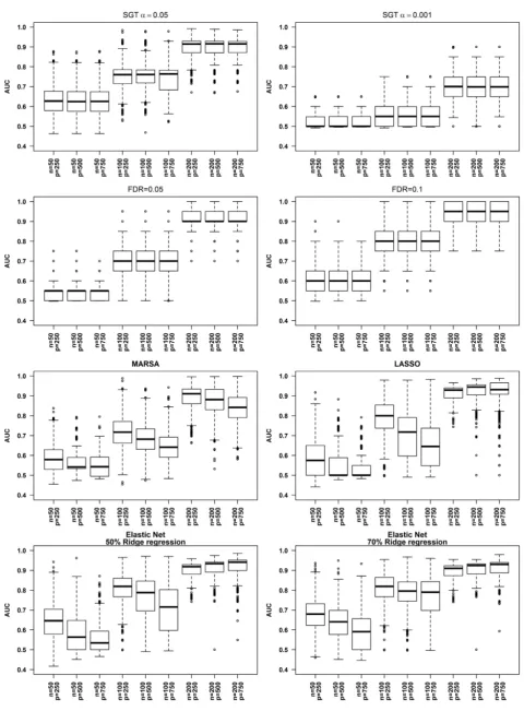
The performance of each of these algorithms depends heavily on the sample size. Regardless of the number of genes entered in the analysis, the AUC is higher for n = 200 than for lower n, while the difference made by the number of genes en-tered in the analysis has a much more modest impact. The number of genes con-sidered for each of these analyses is small in comparison to any high throughput data. This choice is considered realistic as FDR, MARSA and the penalized like-lihood methods are typically applied to a subset of features, chosen through a marginal method as the unadjusted p-value of the SGT method. Figure 4 shows the distributions of the AUC for the 9 situations of Case A for each of the algo-rithms.
Choosing α = 0.001 seems overly conservative with AUC around 0.7 even for n = 200 while for the rest of the algorithms the AUC is around 0.9 for n = 200 and around 0.6 for n = 50. With the exception of the SGT strategy, the other four algorithms exhibit a modest decrease in performance with the number of genes entered in the analysis. The performance increases slightly with the amount of ridge regression included in the Elastic Net. Choosing the genes based on FDR = 0.1 seems to be an excellent choice when the number of observations is adequate. It is important to note that the specificity is in general high (>0.8) and thus the level of AUC depends greatly on the level of sensitivity (Supplementary Tables 1(a)-(c)). In most cases, the sensitivity is tremendously poor (<0.4) for n = 50. This low sensitivity suggests that the sample size is extremely important and ar-gues against dividing an already small dataset into two subsets for training and validation.
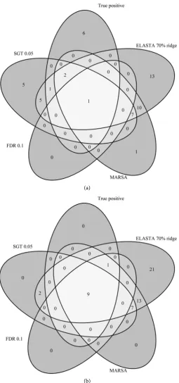
(a)
[image:11.595.248.504.67.613.2](b)
Figure 5. Examples of two datasets and the number of selected genes by each algorithm: (a) the number of records is 50; (b) the number of records is 200.
0.05. However, the number of genes selected by at least one of the algorithms but not associated with the outcome is quite large (43).
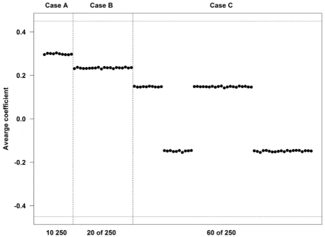
It was observed that the estimated coefficients for each strategy are sometimes biased, depending on the number of genes theoretically associated with outcome and on the correlation structure between these genes (Figure 6). When the genes were independent of each other, the estimated coefficients were always smaller in absolute value than the theoretical coefficient. As the number of genes asso-ciated with the outcome increased, the estimated coefficients were further from the theoretical value. Figure 6 presents the averages over the 2000 simulations of the estimated coefficients (based on SGT) when 10, 20 and 60 genes were asso-ciated with the outcome. In this figure all genes were independent of each other. The horizontal lines are drawn at the theoretical coefficients of ±0.45. The thicker vertical broken lines divide the different datasets.
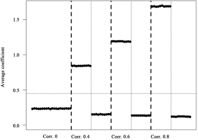
The coefficients obtained from SGT for the correlated genes were biased away from the null while for those uncorrelated (but in the presence of some corre- lated genes) the bias was slightly towards the null (Figure 7 for Case B and Sup-plementary Figure 1 for Case C).
[image:12.595.209.535.463.700.2]Thus, in the presence of correlated genes, the overall performance is mislead- ing as it will average the performance of the correlated genes more likely to be selected with the performance of the uncorrelated genes less likely to be selected. Table 2 shows the sensitivity for Case B for the two groups of genes: 10 corre-lated and 10 independent. As expected, the SGT algorithms have a sensitivity of 1 when the genes were correlated, but the sensitivity was very poor when the genes were independent. Note that for the SGT algorithms even a poor correla-tion like 0.4 can have a tremendous effect on the significance of the correlated
Table 2. The sensitivity for Case B.
SGT
MARSA Penalized likelihood α = 0.05 α = 0.001 FDR = 0.05 FDR = 0.1 LASSO ELASTA5* ELASTA3**
CCorrelation 0 10 genes 0.649 0.17 0.554 0.702 0.692 0.85 0.852 0.854
10 genes 0.654 0.171 0.564 0.71 0.696 0.853 0.856 0.857
Correlation 0.4 10 correlated genes 1 1 1 1 0.585 0.981 0.994 0.998
10 independent genes 0.334 0.04 0.106 0.227 0.551 0.588 0.596 0.598
Correlation 0.6 10 correlated genes 1 1 1 1 0.479 0.955 0.986 0.996
10 independent genes 0.274 0.026 0.045 0.128 0.493 0.515 0.524 0.528
Correlation 0.8 10 correlated genes 1 1 1 1 0.331 0.874 0.97 0.994
10 independent genes 0.224 0.018 0.019 0.069 0.443 0.459 0.47 0.473
*Elastic Net with 50% ridge regression. **Elastic Net with 70% ridge regression.
Figure 7. The average of the coefficients for the first the 20 genes associated with out-come (10 correlated among themselves and 10 independent) over the 2000 simulations for Case B.
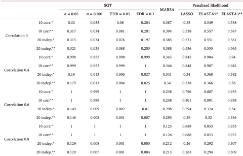
gene. On the other hand, the LASSO and Elastic Net algorithms perform better than MARSA and almost as well as the SGT algorithms for the correlated genes and about the same as MARSA for the uncorrelated genes. The pattern is the same for the Case C (Supplementary Table 2) and the direction of the associa-tion with outcome has no influence on the sensitivity.
6. Conclusions
[image:13.595.210.539.291.523.2]knowledge are at the patient level as well as the social and economic level. How-ever, extracting this information from a large amount of data can be challenging. Several statistical algorithms exist which attempt to find important genetic fea-tures to describe a specific condition or to explain an outcome. This paper presents a comparison of three major strategies for feature selection with surviv-al as outcome. The SGT strategy is present either as the main strategy or as part of a more elaborate algorithm in the majority of papers analyzing high- throughput data. The alpha level of 0.001 is considered more informative as it guards against inflated type I error, ubiquitous in this type of data. This paper also presents the results for an alpha level of 0.05 which is traditionally used in medical statistics as well as 2 levels for FDR (0.05 and 0.1). As the need for more elaborate techniques increases, the LASSO/Elastic Net technique gains populari-ty. It was created specifically to mitigate the disparity between the large number of covariates included in a model and the relatively small number of observa-tions. MARSA is an algorithm created in Princess Margaret Cancer Centre to obtain a genetic signature which explains the difference in survival for appar-ently homogeneously non-small cell lung cancer patients. While not widely used, this algorithm proved to be valuable as the genetic signature found with this technique was successfully validated in independent datasets.
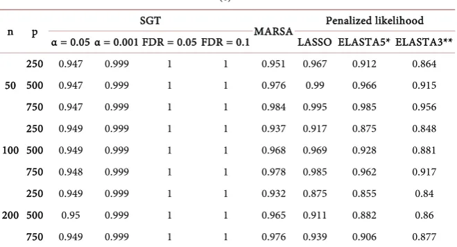
Using simulated data the AUC and the sensitivity for each method under sev-eral scenarios are calculated and presented, suggesting under which conditions each of these strategies is most beneficial. The specificity (for case A, Supple-mentary Table 1(c)) is high in general due to the large number of genes gener-ated under the null hypothesis (no association with survival).
To replicate realistic datasets, several parameters were varied in the process of simulation: the number of observations, the number of genes entered in the al-gorithm, the number of associated genes, the strength and the direction of asso-ciations of the genes with survival and the level of the correlation between genes. The combination of the different sample sizes, the different strengths of associa-tion with survival and the level of significance, α, covers a wide range of the sta-tistical power with which a gene can be detected (15% to 99%).
Our simulations indicate that the number of observations is extremely impor-tant when analyzing this type of data. Thus, regardless of the chosen strategy or number of genes the AUC is higher when the sample size is 200. The ability to select the correct genes is affected by the number of genes when MARSA or one of the Elastic Net methods is used. Therefore, there is no real advantage to divide a small dataset into two very small datasets to obtain training and validation da-tasets. A far better choice is to obtain another independent sample on which to validate the results. Increasingly, datasets with genetic and outcome information can be found in the public domain, and can be used for validation. In the ab-sence of such a dataset, applying more than one method and utilizing a cross- validation technique might help in choosing the appropriate algorithm.
be lower than the theoretical coefficients. This attenuation implies that the SGT technique is unlikely to select these genes and an algorithm which considers more genes at the same time in the model is more desirable (like MARSA or pe-nalized likelihood). On the other hand, the correlation between genes (even a poor correlation of 0.4), when each one of them contributes to the outcome, could make each gene appear more interesting than it really is, due to an overes-timation of the real coefficient. Thus, the correlations between the genes which are entered into MARSA or penalized likelihood need to be calculated.
As in any simulation study, it was possible to judge the efficiency of a method because we had information on the true underlying relationship in the data, in-formation which is not usually available in the process of analyzing a real data-set. However, this study could give information on how these methods behave such that one could interpret the results easier.
It was not considered necessary to present examples as each of these strategies has been applied to real datasets in the past. Moreover, the main objective for this paper was to determine the suitability of these strategies in correctly select-ing as many of the associated genes as possible. The underlyselect-ing assumption is that the appropriate set of features would also validate in an independent study. In addition, we do not wish to recommend a specific strategy for use in all situa-tions as, indeed, this is unrealistic, but present situasitua-tions when each of these strategies may be more suitable than another. We also recommend that any new strategy needs to be thoroughly investigated in simulated environment and eva-luated against other common strategies.
In conclusion, one has to employ not only methodologies which test for asso-ciation with outcome but also for correlations between the features considered. This paper is intended to guide a statistician or bioinformatician in the daunting task of finding genes associated with outcome.
Competing Interests
The authors declare that they have no competing interests. None of the authors have any financial competing interests to disclose.
Authors’ Contribution
MP: initiated the research, performed statistical analysis, drew conclusions, drafted the manuscript
JS: drew conclusions, critically revised the manuscript. All authors read and approved the final manuscript.
References
[1] Potti, A., Mukherjee, S., Petersen, R., Dressman, H.K., Bild, A., Koontz, J., et al.
(2006) A Genomic Strategy to Refine Prognosis in Early-Stage Non-Small-Cell Lung Cancer. The New England Journal of Medicine, 355, 570-580. (Retracted Article, 2007, 356, 201)
Adenocarci-noma. Clinical Cancer Research, 14, 5565-5570.
https://doi.org/10.1158/1078-0432.CCR-08-0544
[3] Chen, G., Kim, S., Taylor, J.M.G., Wang, Z., Lee, O., Ramnath, N., et al. (2011) De-velopment and Validation of a Quantitative Real-Time Polymerase Chain Reaction Classifier for Lung Cancer Prognosis. Journal of Thoracic Oncology, 6, 1481-1487.
https://doi.org/10.1097/JTO.0b013e31822918bd
[4] Bueno, R., Hughes, E., Wagner, S., Gutin, A.S., Lanchbury, J.S., Zheng, Y., et al.
(2015) Validation of a Molecular and Pathological Model for Five-Year Mortality Risk in Patients with Early Stage Lung Adenocarcinoma. Journal of Thoracic On-cology, 10, 67-73. https://doi.org/10.1097/JTO.0000000000000365
[5] Zhu, C., Ding, K., Strumpf, D., Weir, B.A., Meyerson, M., Pennell, N., et al. (2010) Prognostic and Predictive Gene Signature for Adjuvant Chemotherapy in Resected Non-Small-Cell Lung Cancer. Journal of Clinical Oncology, 28, 4417-4424.
https://doi.org/10.1200/JCO.2009.26.4325
[6] Tibshirani, R. (1997) The Lasso Method for Variable Selection in the Cox Model.
Statistics in Medicine, 16, 385-395.
https://doi.org/10.1002/(sici)1097-0258(19970228)16:4<385::aid-sim380>3.0.co;2-3
[7] Zou, H. and Hastie, T. (2005) Regularization and Variable Selection via the Elastic Net. Journal of the Royal Statistical Society Series B—Statistical Methodology, 67, 301-320. https://doi.org/10.1111/j.1467-9868.2005.00503.x
[8] Song, Q. and Liang, F. (2015) A Split-and-Merge Bayesian Variable Selection Ap-proach for Ultrahigh Dimensional Regression. Journal of the Royal Statistical So-ciety Series B—Statistical Methodology, 77, 947-972.
https://doi.org/10.1111/rssb.12095
[9] Zhu, C., Strumpf, D., Li, C., Li, Q., Liu, N., Der, S., et al. (2010) Prognostic Gene Expression Signature for Squamous Cell Carcinoma of Lung. Clinical Cancer Re-search, 16, 5038-5047. https://doi.org/10.1158/1078-0432.CCR-10-0612
[10] Pavlou, M., Ambler, G., Seaman, S., De Iorio, M. and Omar, R.Z. (2016) Review and Evaluation of Penalised Regression Methods for Risk Prediction in Low-Dimensional Data with Few Events. Statistics in Medicine, 35, 1159-1177.
https://doi.org/10.1002/sim.6782
[11] Buehlmann, P. and Mandozzi, J. (2014) High-Dimensional Variable Screening and Bias in Subsequent Inference, with an Empirical Comparison. Computational Sta-tistics, 29, 407-430. https://doi.org/10.1007/s00180-013-0436-3
[12] Cox, D.R. (1972) Regression Models and Life-Tables. Journal of the Royal Statistical Society Series B—Statistical Methodology, 34, 187.
[13] Simon, R.M., Korn, E.L., McShane, L.M., Radmacher, M.D., Wright, G.W. and Zhao, Y. (2003) Design and Analysis of DNA Microarray Investigations. Springer- Verlag, New York.
[14] Benjamini, Y. and Hochberg, Y. (1995) Controlling the False Discovery Rate—A Practical and Powerful Approach to Multiple Testing. Journal of the Royal Statistic-al Society Series B—Methodological, 57, 289-300.
[15] Aben, N., Vis, D.J., Michaut, M. and Wesseis, L.F.A. (2016) TANDEM: A Two- Stage Approach to Maximize Interpretability of Drug Response Models Based on Multiple Molecular Data Types. Bioinformatics, 32, 413-420.
https://doi.org/10.1093/bioinformatics/btw449
[16] Aguirre-Gamboa, R., Martinez-Ledesma, E., Gomez-Rueda, H., Palacios, R., Fuentes- Hernandez, I., Sanchez-Canales, E., et al. (2016) Efficient Gene Selection for Cancer Prognostic Biomarkers Using Swarm Optimization and Survival Analysis. Current
[17] Algamal, Z.Y., Lee, M.H. and Al-Fakih, A.M. (2016) High-Dimensional Quantita-tive Structure-Activity Relationship Modeling of Influenza Neuraminidase a/PR/8/34 (H1N1) Inhibitors Based on a Two-Stage Adaptive Penalized Rank Re-gression. Journal of Chemometrics, 30, 50-57. https://doi.org/10.1002/cem.2766
[18] Amene, E., Hanson, L.A., Zahn, E.A., Wild, S.R. and Dopfer, D. (2016) Variable Se-lection and Regression Analysis for the Prediction of Mortality Rates Associated with Foodborne Diseases. Epidemiology & Infection, 144, 1959-1973.
https://doi.org/10.1017/S0950268815003234
[19] Blomfeldt, A., Aamot, H.V., Eskesen, A.N., Monecke, S., White, R.A., Leegaard, T.M., et al. (2016) DNA Microarray Analysis of Staphylococcus aureus Causing Bloodstream Infection: Bacterial Genes Associated with Mortality? European Jour-nal of Clinical Microbiology & Infectious Diseases, 35, 1285-1295.
https://doi.org/10.1007/s10096-016-2663-3
[20] Bowman, F.D., Drake, D.F. and Huddleston, D.E. (2016) Multimodal Imaging Sig-natures of Parkinson’s Disease. Frontiers in Neuroscience, 10, 131.
https://doi.org/10.3389/fnins.2016.00131
[21] Badsha, M.B., Kurata, H., Onitsuka, M., Oga, T. and Omasa, T. (2016) Metabolic Analysis of Antibody Producing Chinese Hamster Ovary Cell Culture under Dif-ferent Stresses Conditions. Journal of Bioscience and Bioengineering, 122, 117- 124.
https://doi.org/10.1016/j.jbiosc.2015.12.013
[22] Cui, Y., Song, J., Pollom, E., Alagappan, M., Shirato, H., Chang, D.T., et al. (2016) Quantitative Analysis of F-18-Fluorodeoxyglucose Positron Emission Tomography Identifies Novel Prognostic Imaging Biomarkers in Locally Advanced Pancreatic Cancer Patients Treated with Stereotactic Body Radiation Therapy. International Journal of Radiation Oncology Biology Physics, 96, 102-109.
https://doi.org/10.1016/j.ijrobp.2016.04.034
[23] De Vos, F., Schouten, T.M., Hafkemeijer, A., Dopper, E.G.P., van Swieten, J.C., de Rooij, M., et al. (2016) Combining Multiple Anatomical MRI Measures Improves Alzheimer’s Disease Classification. Human Brain Mapping, 37, 1920-1929.
https://doi.org/10.1002/hbm.23147
[24] Frost, H.R., Shen, L., Saykin, A.J., Williams, S.M., Moore, J.H. and The Alzheimer’s Disease Neuroimaging Initiative (2016) Identifying Significant Gene-Environment Interactions Using a Combination of Screening Testing and Hierarchical False Dis-covery Rate Control. Genetic Epidemiology, 40, 544-557.
https://doi.org/10.1002/gepi.21997
[25] Gim, J., Cho, Y.B., Hong, H.K., Kim, H.C., Yun, S.H., Wu, H., et al. (2016) Predict-ing Multi-Class Responses to Preoperative Chemoradiotherapy in Rectal Cancer Pa-tients. Radiation Oncology, 11, 50.
https://doi.org/10.1186/s13014-016-0623-9
[26] Gong, H., Zhang, S., Wang, J., Gong, H. and Zeng, J. (2016) Constructing Structure Ensembles of Intrinsically Disordered Proteins from Chemical Shift Data. Journal of Computational Biology, 23, 300-310. https://doi.org/10.1089/cmb.2015.0184
[27] Hwang, W., Choi, J., Kwon, M. and Lee, D. (2016) Context-Specific Functional Module Based Drug Efficacy Prediction. BMC Bioinformatics, 17, 275.
https://doi.org/10.1186/s12859-016-1078-6
[28] Iniesta, R., Malki, K., Maier, W., Rietschel, M., Mors, O., Hauser, J., et al. (2016) Combining Clinical Variables to Optimize Prediction of Antidepressant Treatment Outcomes. Journal of Psychiatric Research, 78, 94-102.
https://doi.org/10.1016/j.jpsychires.2016.03.016
(2016) Changes in Expression of Genes Representing Key Biologic Processes after Neoadjuvant Chemotherapy in Breast Cancer, and Prognostic Implications in Re-sidual Disease. Clinical Cancer Research, 22, 2405-2416.
https://doi.org/10.1158/1078-0432.CCR-15-1488
[30] Knight, A.K., Craig, J.M., Theda, C., Baekvad-Hansen, M., Bybjerg-Grauholm, J., Hansen, C.S., et al. (2016) An Epigenetic Clock for Gestational Age at Birth Based on Blood Methylation Data. Genome Biology, 17, 206.
https://doi.org/10.1186/s13059-016-1068-z
[31] Lenters, V., Portengen, L., Rignell-Hydbom, A., Jonsson, B.A.G., Lindh, C.H., Piersma, A.H., et al. (2016) Prenatal Phthalate, Perfluoroalkyl Acid, and Organoch-lorine Exposures and Term Birth Weight in Three Birth Cohorts: Multi-Pollutant Models Based on Elastic Net Regression. Environmental Health Perspectives, 124, 365-372.
[32] Leung, J.M., Chen, V., Hollander, Z., Dai, D., Tebbutt, S.J., Aaron, S.D., et al. (2016) COPD Exacerbation Biomarkers Validated Using Multiple Reaction Monitoring Mass Spectrometry. PLoS ONE, 11, e0161129.
https://doi.org/10.1371/journal.pone.0161129
[33] Li, Z., Tang, J. and Guo, F. (2016) Identification of 14-3-3 Proteins Phosphopeptide- Binding Specificity Using an Affinity-Based Computational Approach. PLoS ONE, 11, e0147467. https://doi.org/10.1371/journal.pone.0147467
[34] Martin, O., Ahedo, V., Ignacio, S.J., De Tiedra, P. and Manuel, G.J. (2016) Quality Assessment of Resistance Spot Welding Joints of AISI 304 Stainless Steel Based on Elastic Nets. Materials Science and Engineering A—Structural Materials Properties Microstructure and Processing, 676, 173-181.
https://doi.org/10.1016/j.msea.2016.08.112
[35] Park, J., Kim, J.H., Seo, E., Bae, D.H., Kim, S., Lee, H., et al. (2016) Identification and Evaluation of Age-Correlated DNA Methylation Markers for Forensic Use. Fo-rensic Science International-Genetics, 23, 64-70.
https://doi.org/10.1016/j.fsigen.2016.03.005
[36] Pineda, S., Real, F.X., Kogevinas, M., Carrato, A., Chanock, S.J., Malats, N., et al.
(2015) Integration Analysis of Three Omics Data Using Penalized Regression Me-thods: An Application to Bladder Cancer. PLOS Genetics, 11, e1005689.
https://doi.org/10.1371/journal.pgen.1005689
[37] Reps, J.M., Aickelin, U. and Hubbard, R.B. (2016) Refining Adverse Drug Reaction Signals by Incorporating Interaction Variables Identified Using Emergent Pattern Mining. Computers in Biology and Medicine, 69, 61-70.
https://doi.org/10.1016/j.compbiomed.2015.11.014
[38] Shahabi, A., Lewinger, J.P., Ren, J., April, C., Sherrod, A.E., Hacia, J.G., et al. (2016) Novel Gene Expression Signature Predictive of Clinical Recurrence after Radical Prostatectomy in Early Stage Prostate Cancer Patients. Prostate, 76, 1239-1256.
https://doi.org/10.1002/pros.23211
[39] Sokolov, A., Carlin, D.E., Paull, E.O., Baertsch, R. and Stuart, J.M. (2016) Path-way-Based Genomics Prediction Using Generalized Elastic Net. PLOS Computa-tional Biology, 12, e1004790. https://doi.org/10.1371/journal.pcbi.1004790
[40] Tapak, L., Mahjub, H., Sadeghifar, M., Saidijam, M. and Poorolajal, J. (2016) Pre-dicting the Survival Time for Bladder Cancer Using an Additive Hazards Model in Microarray Data. Iranian Journal of Public Health, 45, 239-248.
[41] Trzepacz, P.T., Hochstetler, H., Yu, P., Castelluccio, P., Witte, M.M., Dell’Agnello,
G., et al. (2016) Relationship of Hippocampal Volume to Amyloid Burden across
[42] Ueki, M., Tamiya, G. and Alzheimer’s Disease Neuroimaging Initiative (2016) Smooth-Threshold Multivariate Genetic Prediction with Unbiased Model Selection.
Genetic Epidemiology, 40, 233-243. https://doi.org/10.1002/gepi.21958
[43] Yabu, J.M., Siebert, J.C. and Maecker, H.T. (2016) Immune Profiles to Predict Re-sponse to Desensitization Therapy in Highly HLA-Sensitized Kidney Transplant Candidates. PLoS ONE, 11, e0153355. https://doi.org/10.1371/journal.pone.0153355
[44] Yang, R., Xiong, J., Deng, D., Wang, Y., Liu, H., Jiang, G., et al. (2016) An Inte-grated Model of Clinical Information and Gene Expression for Prediction of Sur-vival in Ovarian Cancer Patients. Translational Research, 172, 84-95.
https://doi.org/10.1016/j.trsl.2016.03.001
[45] Yuan, H., Paskov, I., Paskov, H., Gonzalez, A.J. and Leslie, C.S. (2016) Multitask Learning Improves Prediction of Cancer Drug Sensitivity. Scientific Reports, 6, Ar-ticle No. 31619. https://doi.org/10.1038/srep31619
[46] Simon, N., Friedman, J., Hastie, T. and Tibshirani, R. (2011) Regularization Paths for Cox’s Proportional Hazards Model via Coordinate Descent. Journal of Statistical Software, 39, 1-13.
[47] Verweij, P.J.M. and Vanhouwelingen, H.C. (1993) Cross-Validation in Survival Analysis. Statistics in Medicine, 12, 2305-2314.
[48] Der, S.D., Sykes, J., Pintilie, M., Zhu, C., Strumpf, D., Liu, N., et al. (2014) Valida-tion of a Histology-Independent Prognostic Gene Signature for Early-Stage, Non-Small-Cell Lung Cancer Including Stage IA Patients. Journal of Thoracic On-cology, 9, 59-64.
Supplementary
Table 1. (a) The average AUC for each scenario of Case A; (b) The average sensitivity for each scenario of Case A; (c) The average specificity for each scenario of Case A.
(a)
n p SGT MARSA Penalized likelihood
α = 0.05 α = 0.001 FDR = 0.05 FDR = 0.1 LASSO ELASTA5* ELASTA3**
50
250 0.634 0.517 0.542 0.601 0.585 0.588 0.644 0.675 500 0.631 0.517 0.54 0.602 0.56 0.548 0.585 0.638 750 0.633 0.517 0.541 0.598 0.551 0.533 0.554 0.594
100
250 0.752 0.557 0.709 0.789 0.716 0.783 0.805 0.808 500 0.751 0.556 0.705 0.788 0.675 0.698 0.756 0.794 750 0.748 0.556 0.702 0.785 0.652 0.646 0.7 0.756
200
250 0.899 0.687 0.914 0.95 0.894 0.914 0.905 0.897 500 0.897 0.683 0.912 0.948 0.873 0.927 0.916 0.907 750 0.896 0.683 0.911 0.949 0.853 0.926 0.92 0.911 *Elastic net with 50% ridge regression; **Elastic net with 70% ridge regression.
(b)
n p SGT MARSA Penalized likelihood
α = 0.05 α = 0.001 FDR = 0.05 FDR = 0.1 LASSO ELASTA5* ELASTA3**
50
250 0.322 0.034 0.083 0.203 0.218 0.208 0.377 0.486 500 0.314 0.036 0.079 0.204 0.145 0.106 0.205 0.361 750 0.32 0.035 0.082 0.197 0.118 0.071 0.123 0.232
100
250 0.555 0.114 0.418 0.578 0.496 0.65 0.734 0.767 500 0.553 0.114 0.411 0.576 0.382 0.428 0.584 0.708 750 0.548 0.113 0.404 0.571 0.326 0.307 0.438 0.596
200
250 0.848 0.374 0.828 0.901 0.856 0.954 0.955 0.955 500 0.844 0.368 0.823 0.895 0.781 0.943 0.95 0.953 750 0.843 0.367 0.822 0.897 0.73 0.912 0.935 0.944 *Elastic net with 50% ridge regression; **Elastic net with 70% ridge regression.
(c)
n p SGT MARSA Penalized likelihood
α = 0.05 α = 0.001 FDR = 0.05 FDR = 0.1 LASSO ELASTA5* ELASTA3**
50
250 0.947 0.999 1 1 0.951 0.967 0.912 0.864
500 0.947 0.999 1 1 0.976 0.99 0.966 0.915
750 0.947 0.999 1 1 0.984 0.995 0.985 0.956
100
250 0.949 0.999 1 1 0.937 0.917 0.875 0.848
500 0.949 0.999 1 1 0.968 0.969 0.928 0.881
750 0.948 0.999 1 1 0.978 0.985 0.962 0.917
200
250 0.949 0.999 1 1 0.932 0.875 0.855 0.84
500 0.95 0.999 1 1 0.965 0.911 0.882 0.86
750 0.949 0.999 1 1 0.976 0.939 0.906 0.877
Figure 1. Average of the coefficients over the 2000 simulations for the 60 genes associated with outcome with the first 20 being correlated.
Table 2. The sensitivity for all scenarios of Case C.
SGT
MARSA Penalized likelihood α = 0.05 α = 0.001 FDR = 0.05 FDR = 0.1 LASSO ELASTA5* ELASTA3**
Correlation 0
10 corr.* 0.32 0.033 0.08 0.204 0.387 0.53 0.549 0.558
10 corr** 0.317 0.034 0.081 0.201 0.394 0.538 0.557 0.567
20 indep.* 0.315 0.034 0.076 0.197 0.385 0.531 0.551 0.561
20 indep.** 0.321 0.035 0.088 0.203 0.388 0.536 0.555 0.565
Correlation 0.4
10 corr.* 0.998 0.955 0.998 0.999 0.343 0.845 0.904 0.94
10 corr** 0.999 0.952 0.999 1 0.346 0.848 0.907 0.942
20 indep.* 0.18 0.013 0.006 0.027 0.341 0.34 0.368 0.382
20 indep.** 0.179 0.013 0.004 0.025 0.34 0.338 0.366 0.38
Correlation 0.6
10 corr.* 1 0.999 1 1 0.238 0.796 0.887 0.935
10 corr** 1 0.999 1 1 0.238 0.801 0.891 0.938
20 indep.* 0.149 0.009 0.002 0.01 0.298 0.294 0.324 0.34
20 indep.** 0.148 0.008 0.001 0.007 0.295 0.29 0.32 0.336
Correlation 0.8
10 corr.* 1 1 1 1 0.125 0.688 0.853 0.933
10 corr** 1 1 1 1 0.126 0.688 0.853 0.932
20 indep.* 0.129 0.008 0.001 0.005 0.212 0.26 0.292 0.307
20 indep.** 0.129 0.007 0.001 0.004 0.213 0.263 0.294 0.309
*Theoretical coefficient is 0.45; **Theoretical coefficient is (−0.45).
-0.5 0.0 0.5
A
vear
g
e co
ef
fi
ci
en
t
[image:21.595.56.537.337.644.2]List of Abbreviations
AUC = Area Under the Receiver Operating Characteristic Curve SGT = Single Gene Testing
LASSO = Least Absolute Shrinkage and Selection Operator MARSA = Maximizing R Square Algorithm
LRT = Likelihood Ratio Test FDR = False Discovery Rate PCR = Polymerase Chain Reaction
Submit or recommend next manuscript to SCIRP and we will provide best service for you:
Accepting pre-submission inquiries through Email, Facebook, LinkedIn, Twitter, etc. A wide selection of journals (inclusive of 9 subjects, more than 200 journals)
Providing 24-hour high-quality service User-friendly online submission system Fair and swift peer-review system
Efficient typesetting and proofreading procedure
Display of the result of downloads and visits, as well as the number of cited articles Maximum dissemination of your research work
Submit your manuscript at: http://papersubmission.scirp.org/