Semi supervised deep rule based approach for image classification

Semi-supervised Deep Rule-based Approach for Image Classification

Xiaowei Gu1 and Plamen P. Angelov1,2* 1

School of Computing and Communications, Lancaster University, Lancaster, LA1 4WA, UK 2_{Technical University, Sofia, 1000, Bulgaria (Honorary Professor)}

e-mail: {x.gu3, p.angelov}@lancaster.ac.uk

Abstract- In this paper, a semi-supervised learning approach based on a deep rule-based (DRB) classifier is introduced. With its unique prototype-based nature, the semi-supervised DRB (SSDRB) classifier is able to generate human interpretable IF…THEN… rules through the semi-supervised learning process in a self-organising and highly transparent manner. It supports online learning on a sample-by-sample basis or on a chunk-by-chunk basis. It is also able to perform classification on out-of-sample images. Moreover, the SSDRB classifier can learn new classes from unlabelled images in an active way becoming dynamically self-evolving. Numerical examples based on large-scale benchmark image sets demonstrate the strong performance of the proposed SSDRB classifier as well as its distinctive features compared with the “state-of-the-art” approaches. Keywords- semi-supervised learning; deep rule-based (DRB) classifier; prototype-based models; fuzzy rules; self-organising classifier; transparency and interpretability.

1. Introduction

Due to the more accessible electronics and the boom in the information technologies, an astronomic amount of images are being produced and uploaded on the web every day. Studying and classifying these images is of paramount importance [1]. Facing the strong demand, however, traditional fully supervised machine learning approaches are insufficient [2], [3]. In most real applications, labelled images are scarce and it is expensive to obtain them. Despite the fact that unlabelled images are abundant, supervised approaches are not able to effectively use them.

Semi-supervised machine learning approaches [4]–[9] consider both the labelled and unlabelled data. The goal of the semi-supervised learning is to use the unlabelled data to improve the generalisation. Cluster assumption states that the decision boundary should not cross high density regions, but lie in low density regions [6]. Virtually all the existing successful semi-supervised approaches rely on the cluster assumption in a direct or indirect way from estimating or optimizing a smooth classification function over labelled and unlabelled data [10], [11].

There are two major branches of semi-supervised approaches, SVM-based and graph-based approaches [8], [12]. Semi-supervised SVMs [13]–[15] are extensions of the traditional SVMs [2] to a semi-supervised scenario. Traditional SVMs maximise the separation between classes based on the training data via a maximum-margin hyperplane [2], while semi-supervised classifiers balance the estimated maximum-maximum-margin hyperplane with a separation of all the data through the low-density regions. Graph-based approaches [8], [12], [16] use the labelled and unlabelled data as vertices in a graph and build pairwise edges between the vertices weighted by similarities. In general, both types of semi-supervised approaches are computationally expensive and they consume a lot of computer memory, thus, are not suitable for large-scale datasets. Moreover, they are not applicable to the out-of-sample data and require full retraining when more training samples are given [12].

In addition to the two main branches, the idea of “pseudo label” also has been exploited by some semi-supervised approaches [17]–[19]. This kind of approaches start the semi-semi-supervised learning by enlarging the training set with the pseudo-labelled samples, which are selected from the unlabelled data based on the characteristic of the labelled ones. Then, they train a genetic algorithm, i.e. fuzzy SVM [17], neural network [19], with a hybrid of labelled and pseudo-labelled data. However, because the employed genetic algorithm requires a full retraining if more labelled and/or pseudo-labelled data is given, the current pseudo label-based approaches are limited to offline applications. In addition, due to the iterative computation process of the genetic algorithms, the accuracy of pseudo-labelling can largely influence the performance of these approaches.

[20]–[22]. The “core” of the DRB classifier is formed by IF…THEN… rules, which consist of a number of prototypes. These can be represented as a series of simpler fuzzy rules with a single prototype connected by a logical “OR” operator [22]. The prototypes are identified from the training data directly in a nonparametric, self-organising way, and they are the most representative prototypes standing for the local maxima of data density [23].

This paper further extends the DRB classifier with a self-organising, self-evolving semi-supervised learning strategy by exploiting the idea of “pseudo label” naturally with its prototype-based nature. Starting with a small amount of labelled training images, the semi-supervised DRB (SSDRB) classifier is able to pseudo-label remaining images based on the ensemble properties of the training images using nonparametric measures [23]. Without a full retraining, the SSDRB classifier can self-organise its system structure and self-update meta-parameters recursively with the pseudo-labelled data and thus, it supports real-time streaming data processing. The proposed SSDRB classifier also inherits the advantage of transparency of the DRB classifier as its semi-supervised learning process only concerns the visual similarity between the identified prototypes and the unlabelled samples, which is highly human interpretable compared with the state-of-the-art approaches, i.e. SVM [2] and deep learning networks [24].

The proposed SSDRB classifier not only can perform classification on out-of-sample images, but also support recursive online training on a sample-by-sample basis or a chunk-by-chunk basis. Moreover, unlike other semi-supervised approaches, the proposed approach is able to learn new classes actively without human experts’ involvement, thus, to self-evolve [25]. Numerical examples based on large-scale benchmark image sets demonstrate the transparent learning process and the high performance of the proposed SSDRB classifier.

In short, compared with the existing semi-supervised approaches [4]–[8], [10]–[16], the proposed SSDRB classifier has the following distinctive features because of its prototype-based nature [20]–[22]:

1) Its semi-supervised learning process is fully transparent and human-interpretable;

2) It can be trained online on a sample-by-sample or chunk-by-chunk basis;

3) It can classify out-of-sample images;

4) It is able to learn new classes (self-evolve).

The remainder of this paper is organised as follows. Section 2 summarises the architecture, training process and validation of the DRB classifier. The proposed semi-supervised learning strategy for the DRB classifier is introduced in section 3 as the main contribution of this paper. Section 4 presents the numerical examples and section 5 concludes this paper.

2. Deep Rule-based Classifier

In this section, we will briefly describe the architecture, training process and validation of the recently introduced deep rule-based (DRB) [20]–[22] classifier to make this paper self-contained.

2.1. Architecture

Fig.1 Architecture of the DRB classifier considered in this paper

1) Normalisation layer;

This layer normalises the pixel values of the images into the range that the feature descriptor works with. Because of the specific feature descriptor used in this paper, the required range of the pixel values is



0, 255



[26].

2) Scaling layer;

This layer is for resizing the original size of the images for various purposes, i.e. reducing the computational complexity, increasing generalisation, etc. In the DRB classifier used in this paper, all the images are resized to the size of 227 227 pixels [26] because of the specific feature descriptor used.

3) Feature descriptor;

Feature descriptor extracts global feature vectors from the images that will be used for training or testing. Currently, deep convolutional neural networks (DCNNs) have become the state-of-art approach in the image recognition [24]. However, training a DCNN for a specific problem is computationally expensive and requires a lot of labelled training samples [22]. However, to perform classification using a pre-trained DCNN on a new problem at which the DCNN is not targeted, human expertise and efforts are heavily needed for fine-tuning. A widely used alterative approach is to use the pre-trained DCNN to extract global features from the training images, and use these feature vectors to train a genetic classifier [22], [27]. By using the pre-trained DCNN as descriptor, the classifier can learn more abstract and discriminative high-level features and achieve greater accuracy.

Following this concept, in this work, the pre-trained vgg-verydeep-16 DCNN [26] is employed for feature extraction because of its simper structure and better performance. The 1 4096 dimensional activations from the first fully connected layer are used as the feature vector of the image [27]. This helps avoid handcrafting and automates the whole process.

4) Fuzzy rule base (FRB) layer [20]–[22];

The C AnYa type FRB subsystems are entirely independent from each other, and each of them can be changed without influencing others. Each FRB subsystem contains a set of massively parallel AnYa type 0-order fuzzy rules formulated around the prototypes (which are the local peaks of data density [23]) identified during the training stage from the images of the corresponding class based on their feature vectors. These 0-order AnYa type fuzzy rules have the following form:



~ c







i

IF I P THEN class c (1) where “~” denotes similarity, which can also be seen as a fuzzy degree of satisfaction or membership;

1, 2,..., c C; c

N is the number of prototypes of the cth class; c i

P is the identified prototypes,_i1, 2,...,_Nc_. Since all of them have the same consequence (same class label, c), they can be combined into one rule with multiple conditions linked with logical “OR” operator [22]. This combined fuzzy rule has the following form per class:



~ 1

 

~ 2



...



~ c







c c c

N

IF I P OR I P OR OR I P THEN class c (2) The “winner-takes-all” decision-making principle is used to determine the overall degree of satisfaction, see the zoom-in part of Fig. 1.

During the validation stage, for each testing image, each fuzzy rule generates one score of confidence/ degree of satisfaction using the “winner-takes-all” principle. Then, all the scores of confidence generated by the fuzzy rule base will be passed to the next layer (the decision-maker) for an overall decision for the class label. For a training data set with C classes, there will be C overall (combined) fuzzy rules identified (one rule per class).

5) Decision-maker.

The decision-maker forms the overall decision by assigning labels to the validation images based on the degree of similarity to the prototypes obtained by the FRB layer.

The training process of the FRB layer is summarised in subsection 2.2, and the validation stage including the decision-making mechanism is presented in subsection 2.3.

2.2. Training Process

2.2.1. Algorithm

During the training process, the prototypes are being identified as the peaks of the data density in the feature space [20]–[22]. Based on these prototypes, the corresponding fuzzy rules are generated. Because of the very high dimensionality of the feature vectors, we use cosine dissimilarity as the distance measure, which is given below [30]:





1

,

, 2 2 cos 2 2

M

i i i

x y

d  



    



x y

x y x y

x y x y (3)

where x y, is the angle between feature vectors x and y ;

1 , , cos M i i i x y  _{ }



 x y x y

x y x y ;

2 1 , M i i x   



x x x denotes the norm of x, M is the dimensionality of the vector; in our case, M 4096.

It has been demonstrated in [30] that the cosine dissimilarity between the original vectors of the global features is equivalent to the Euclidean distance between the vectors normalised by their norms (x x

As the training process can be done in parallel for each fuzzy rule, we consider the cth (c=1,2,…,C) massively parallel fuzzy rule and summarise its training process as follows.

Stage 0: initialisation

The cth fuzzy rule is initialised by the first image (denoted by ₁c

I ) of the corresponding class with feature vector denoted by 1

c

x (x₁c  x_1,1c,x_1,2c ,...,x_1,c_M_). Then, the meta-parameters of the system are initialised as follows:

1 1 1 1 1 1 1

1; c 1; c c; c c; c c; c 1; c o

k N  P I  x p x S  r r (4) where k is the current time instance; Ncis the number of prototypes; 1

c

P is the first image prototype of the fuzzy rule; c

is the global mean of all the feature vectors of the observed images of the cth class; ₁c

p is the mean of feature vectors of the images associated with 1

c

P , which is also the centre of the data cloud initialised by 1

c P ; 1

c

S is the support of the first data cloud; 1 c

r is the radius of the area of influence of the data cloud; r_o is a small value used to stabilise the initial status of the newly identified prototypes. In this paper,

 

2 2 cos 6 0.5176

o

r  



 ; the rationale is that two vectors for which the angle between them is less than 30o or  6 can be regarded as pointing in close/similar directions. The threshold r_o is defined based on the fact that for two vectors with an angle between them smaller than 30 degrees can be regarded as similar. However, we have to stress that r_o is not a problem- or user- specific parameter and it can be defined without prior knowledge, but by common sense only. In general, the higher r_o is, the fewer prototypes will be identified during the training process, the more efficient the DRB classifier will be, but the less details the DRB classifier will learn from the training, and vice versa.

With the first data cloud, the cth fuzzy rule is generated with the prototype 1 c P as:



~ 1







c

IF I P THEN class c (5) Stage 1: system update

For the newly arrived, kth (k k 1) training image ( c k

I ) that belongs to the cth class, the global mean c

 is firstly updated with its feature vector, denoted by c k

x , as follows:

1 1

c c c

k

k

k k



 





x (6)

And we calculate the data densities of c i

p (_i1, 2,...,_Nc_, c

N is the number of identified prototypes) and the feature vector of c

k I , c

k

x according to Empirical Data Analytics framework [23]:

 

   

2 1 2

2

1

; , ,..., ,

1 ,

c c c c c

k N c c D d



  

z z p p p x

z



(7)

where c _Xc c 2  1 c 2 _; c

X is the average norm of feature vectors of the observed images, which is always equal to 1 due to the vector normalisation operation.

In this stage, we update the system structure and meta-parameters to reflect the newly arrived image. Firstly, the following principle is checked to see whether c

k

I is a new prototype [25]:

Condition 1:

 



 



 



 







1,2,..., 1,2,..., max min c c

c c c c

k j k j

j N j N

c k

IF D D OR D D

THEN is a new prototype

   _  _{ } _   _{ }   I

x p x p

(8)

Once Condition 1 is satisfied, c k

I is set to be a new prototype and it initialises a new data cloud:

1; ; ; 1;

c c c c

c c c c c c c c

N k N k N N o

If Condition 1 is not met, we find the nearest prototype to c k

I , denoted by c n

P , by the following equation:









1,2,...,

arg min ,

c

c c c

n j k

j N d  

P p x (10)

Before we associate c k

I to the data cloud of c n

P , Condition 2 is checked to see whether c k

I is within the area of influence of c

n P :

Condition 2: IF d





p x_nc, _kc



r_nc



THEN



I_kc is a new prototype



(11) If Condition 2 is met, it means that c

k

I is out of the influence area of the nearest data cloud, and c k I becomes a new prototype of a new data cloud with meta-parameters initialised by equation (9).

Otherwise, c k

I is assigned to the data cloud formed around the prototype c n

P and the meta-parameters of this data cloud are updated as follows:

 

2



2



1 1 1

1; ; 1

2 2

1 1

c

c c c n c c c c c

n n n c n c k n n n

n n

S

S S r r

S S

     

 

p p + x p (12)

and the prototype c n

P stay the same. Stage 2: fuzzy rule update

Once Stage 1 has been finished, the DRB system will update the fuzzy rule accordingly. Then, the next image is read and the system goes back to Stage 1 to start a new processing cycle.

The training process is summarised in the following pseudo code.

Algorithm 1: Training process of the deep rule-based classifier

While the new feature vector c k

x of the kth image c k

I of the cth class is available i. If (k1) Then

1. Initialise the system using eq. (4);

2. Generate the AnYa type fuzzy rule (eq. (5)); ii. Else

1. Update c

using eq. (6); 2. Calculate D

 

xkc and

 

c j

D p (j1, 2,...,Nc) using eq. (7); 3. If ( Condition 1 is met ) Then

- Initialise a new data cloud using eq. (9); 4. Else

- Find c n

P using eq. (10) - If (Condition 2 is met) Then

* Initialise a new data cloud using eq. (9); - Else

*Update the existing data cloud using eq. (12); - End If

5. End If

6. Update the AnYa type fuzzy rule; iii. End If

End While

2.2.2. Illustrative Example

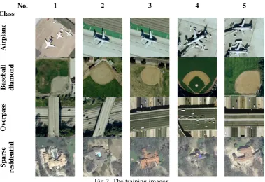
The cosine dissimilarities (d  22 cos) between the feature vectors of the five images within the same class are given in Table 1. The progress of fuzzy rules identification and the final fuzzy rules identified after the training process are given in Tables 2 and 3, respectively.

No. Class

1 2 3 4 5

Airpla

ne

B

a

seba

ll

dia

mo

nd

O

v

er

pa

ss

Sp

a

rse

re

sidentia

l

[image:7.595.109.489.161.421.2]

Fig.2. The training images

Table 1. Cosine dissimilarities between the feature vectors of the five training images of each class.

Airplane Baseball diamond

d 1 2 3 4 5 d 1 2 3 4 5

1 0.9456 0.9456 0.8810 0.9632 1 0.9922 0.9686 1.1294 0.9674

2 0.9456 0.0000 0.8701 1.0044 2 0.9922 0.9384 0.9944 0.9635

3 0.9456 0.0000 0.8701 1.0044 3 0.9686 0.9384 1.1180 0.8963

4 0.8810 0.8701 0.8701 0.7773 4 1.1294 0.9944 1.1180 1.0770

5 0.9632 1.0044 1.0044 0.7773 5 0.9674 0.9635 0.8963 1.0770

Overpass Sparse residential

d 1 2 3 4 5 d 1 2 3 4 5

1 0.7384 0.9539 1.0516 0.8988 1 0.7955 0.8612 0.8888 0.7941

2 0.7384 0.9196 0.9822 0.9398 2 0.7955 0.8342 0.7940 0.7373

3 0.9539 0.9196 0.7895 0.5449 3 0.8612 0.8342 0.7590 0.7487

4 1.0516 0.9822 0.7895 0.8264 4 0.8888 0.7940 0.7590 0.7031

[image:8.595.90.495.82.394.2]

Table 2. AnYa type fuzzy rules identified through the training process Fuzzy rule initialised with the 1st image Fuzzy rule updated with the 2nd image

Fuzzy rule updated with the 3rd image Fuzzy rule updated with the 4th image

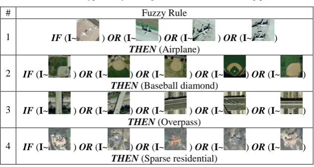
Table 3. AnYa type fuzzy rules generated after the training process

# Fuzzy Rule

1 IF (I~ ) OR (I~ ) OR (I~ ) OR (I~ )

THEN (Airplane)

2 IF (I~ ) OR (I~ ) OR (I~ ) OR (I~ ) OR (I~ ) THEN (Baseball diamond)

3 IF (I~ ) OR (I~ ) OR (I~ ) OR (I~ ) OR (I~ ) THEN (Overpass)

4 IF (I~ ) OR (I~ ) OR (I~ ) OR (I~ ) OR (I~ ) THEN (Sparse residential)

It is important to stress that, because of its prototype-based nature, DRB classifier is able to be trained from a handful of images and is fully transparent (see Tables 2 and 3).

2.3. Validation Process

2.3.1. Algorithm

During the validation process, for each testing image, the C identified fuzzy rules of the DRB classifier will generate C scores of confidence corresponding to the C classes in the training set [22]. For a particular image I with its feature vector denoted by x, the score of confidence of the cth rule within the rule base is given by its local decision-maker as (c=1,2,…,C):

 





2









1,2,...,

max exp ,

c

c c

i i N

d





 

[image:8.595.139.457.425.594.2]

As a result, for each testing image, a vector of 1C dimensional scores of confidence/degrees of closeness to the nearest prototypes (one per class) is generated:

 

1

 

_,...,C

 



  

I I I

 .

The label of this testing image is decided by using the “winner-takes-all” principle [22]:

 





1,2,...,

Label arg max c

c C





 I (14)

2.3.2. Illustrative Example

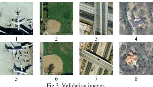
To validate the trained DRB classifier as tabulated in Table 3, we select the eight out-of-sample images given in Fig. 3 from the UCMerced dataset [31]. The scores of confidence/degrees of closeness and the estimated labels of the eight images generated by the four fuzzy rules are given in Table 4, where one can see that the DRB classifier correctly identified the classes of all the eight images.

1 2 3 4

5 6 7 8

[image:9.595.168.428.256.405.2]

Fig.3. Validation images.

Table 4. Scores of confidences of the eight images

3. Semi-supervised Learning

In this section, the semi-supervised learning strategies for the deep-rule-based (DRB) classifier in both offline and online scenarios are introduced. A strategy for the DRB classifier to actively learn new classes from unlabelled training images is also presented. Similar to section 2, illustrative examples will be used to illustrate the concept.

3.1. Semi-supervised Learning Process from Static Datasets

3.1.1. Algorithm

In an offline scenario, all the unlabelled training images are available and the DRB classifier starts to learn from these images after the training process with labelled images finishes. First of all, let us define the

Rule # Image ID

Score of confidence (λ)

Estimated label

1 2 3 4

1 0.5603 0.3752 0.3183 0.3434 Airplane 2 0.2664 0.4836 0.2992 0.3687 Baseball diamond

3 0.3108 0.2824 0.4762 0.2659 Overpass

4 0.3498 0.3468 0.3468 0.6325 Sparse residential 5 0.6286 0.3914 0.3722 0.4110 Airplane 6 0.2852 0.5386 0.3441 0.3632 Baseball diamond

7 0.3505 0.3210 0.5834 0.3333 Overpass

unlabelled training images as the set

 

U , and the number of unlabelled training images as U . The main steps of the semi-supervised learning strategy are described as follows:

Step 1. Extract the vector of scores of confidence/degrees of closeness to the nearest prototypes for each unlabelled training image, denoted by 

 

U_i (i1, 2,...,U), using equation (13).

Step 2. Find out all the unlabelled training images satisfying Condition 3: Condition 3:



*max

 

**max

 





 



0

i i i

IF



U  

 

U THEN U  V (15) where *max

 

i

 U denotes the highest score of confidence U_i obtains, and **max

 

i

 U denotes the second highest score; (



1) is a free parameter;

 

0

V denotes the collection of the unlabelled training images that meet Condition 3. Then

 

0

V is removed from

 

U . For the unlabelled training images

 

0

V that meet Condition 3, the DRB classifier is highly confident about the class these images belong to and they can be used for updating its structure and meta-parameters. Otherwise, it means that the DRB classifier is not highly confident about its judgement and, thus, these images are not used for updating the fuzzy rules.

Compared with other pseudo labelling mechanisms used in other works [17]–[19], Condition 3 considers not only the mutual distances between the unlabelled image and all the identified prototypes, but also the distinguishability of the unlabelled image, which leads to a more accurate pseudo-labelling process.

Step 3. Rank the elements within

 

0

V in a descending order in terms of the values of

 

 



* max **max



V V (

 

0 

V V ), and denote the ranked set as

 

1 V .

As one can see from the definition of the score of confidence equation (13), the higher *max

 

i

 U is, the more similar the image is to a particular prototype of the DRB classifier. Meanwhile, the higher

 

 



* max _**max



V V is, the less ambiguous the decision made by the DRB classifier is. Since the DRB classifier learns sample-by-sample in the form of a data stream, by ranking

 

0

V in advance, the classifier will firstly update itself with images that are more similar to the previously identified prototypes and have less ambiguity in the decisions about their labels, and later with the less familiar ones, which guarantees a more efficient learning.

Step 4. Update the DRB classifier using Algorithm 1 with the set

 

1

V . Then the SSDRB classifier goes back to Step 1 and repeats the whole process, until there are no unlabelled training images that can meet Condition 3.

After the offline semi-supervised learning process is finished, if the DRB classifier is not designed to learn any new classes, the labels of all the unlabelled training images will be estimated using equations (13) and (14) based on the “winner-takes-all” strategy. Otherwise, the DRB classifier will, firstly, produce the pseudo labels of the images that can meet Condition 3 and then, learn new classes through the remaining unlabelled images (will self-evolve).

One distinctive feature of the SSDRB classifier is its robustness to the incorrectly pseudo-labelled images thanks to its prototype-based nature and the “one pass” type (non-iterative) training process. The incorrectly pseudo-labelled images can influence the SSDRB classifier in two ways: 1) they can slightly shift the positions of some of the prototypes; 2) they can create new false prototypes by assigning wrong pseudo-labels (see Algorithm 1).However,the SSDRB classifier has a strong tolerance to a small amount of incorrectly pseudo-labelled images because the errors will not be propagated to the majority of previously existing prototypes in the IF…THEN… rule base (in other words, there is no error propagation).

[image:11.595.171.425.65.377.2]

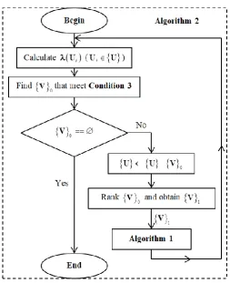
Fig.4. Offline semi-supervised learning process (Algorithm 2)

3.1.2. Illustrative Example

In this subsection, 12 remote sensing images (given in Fig. 5) from the same dataset as in the previous examples are used as the unlabelled training set. These images come from six different classes, nine of them come from the four original classes (“airplane”, “baseball diamond”, “overpass” and “sparse residential”) and three of them come from two new classes (“agricultural” and “harbour”), which are unknown to the DRB classifier trained with the labelled training set as presented in Table 3. The scores of confidence of the 12 images in regards to the four fuzzy rules are tabulated in Table 5, from which we may notice that there are seven images satisfying Condition 3 (in this example, we use



1.2) and the DRB classifier can assign labels to them with high confidence. The rank of the seven images from the illustrative example satisfying Condition 3 is also given in Table 5.

1 2 3 4 5 6

7 8 9 10 11 12

[image:11.595.102.498.575.719.2]

[image:12.595.83.513.106.288.2]

Table 5. Scores of confidence of the unlabelled training images

[image:12.595.79.517.375.566.2]

With the seven images satisfying Condition 3, the original fuzzy rules (as tabulated in Table 2) are updated and new prototypes are added. The updated fuzzy rules are tabulated in Table 6, where the new prototypes are highlighted with red colour.

Table 6. AnYa type fuzzy rules generated through the training process

# Fuzzy Rule

1 IF (I~ ) OR (I~ ) OR (I~ ) OR (I~ )OR (I~ ) OR (I~ )

THEN (Airplane)

2 IF (I~ ) OR (I~ ) OR (I~ ) OR (I~ ) OR (I~ )OR (I~ )

THEN (Baseball diamond)

3 IF (I~ ) OR (I~ ) OR (I~ ) OR (I~ ) OR (I~ )OR (I~ ) OR (I~ )

THEN (Overpass)

4 IF (I~ ) OR (I~ ) OR (I~ ) OR (I~ ) OR (I~ )OR (I~ ) OR (I~ )

THEN (Sparse residential)

Then the algorithm checks the five unlabelled training images left in the second round. The scores of confidence of the five images are given in Table 7. As one can see, because of the first round of the learning process, the DRB classifier is able to recognise another unlabelled image, and the fuzzy rule is updated correspondingly (see Table 8).

Table 7. Scores of confidence of the remaining unlabelled training images Rule #

Image ID

Score of confidence (λ)

Condition 1 Estimated label Rank

1 2 3 4

1 0.3456 0.3309 0.2819 0.3922 No Uncertain

2 0.2867 0.4591 0.3486 0.4107 No Uncertain

3 0.3384 0.2767 0.4725 0.2275 Yes Overpass 5

4 0.3420 0.3808 0.3629 0.6732 Yes Sparse residential 1

5 0.3017 0.2406 0.3159 0.2422 No Uncertain

6 0.3344 0.2732 0.4707 0.2689 Yes Overpass 6

7 0.6448 0.3605 0.3577 0.3897 Yes Airplane 2

8 0.3158 0.4351 0.2810 0.3576 Yes Baseball diamond 7

9 0.2968 0.4054 0.3120 0.6194 Yes Sparse residential 3

10 0.5437 0.2941 0.3602 0.3498 Yes Airplane 4

11 0.3609 0.2775 0.2652 0.3363 No Uncertain

12 0.3437 0.4136 0.3144 0.4124 No Uncertain

Rule # Image ID

Score of confidence (λ)

Condition 1 Estimated label Rank

1 2 3 4

1 0.3456 0.3309 0.2819 0.3922 No Uncertain

2 0.2867 0.4591 0.3486 0.4107 No Uncertain

5 0.3017 0.2492 0.3211 0.2422 No Uncertain

11 0.3774 0.2775 0.2652 0.3363 No Uncertain

[image:12.595.87.511.665.766.2]

[image:13.595.78.519.275.470.2]

Table 8. Updated fuzzy rule after the second round

# Fuzzy Rule

2 IF (I~ ) OR (I~ ) OR (I~ ) OR (I~ ) OR (I~ )OR (I~ ) OR (I~ )

THEN (Baseball diamond)

3.2. Learning New Classes Actively

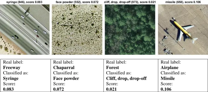
In real situations, the labelled training samples may fail to include all the classes due to various reasons, i.e. an insufficient prior knowledge or change of the data pattern. For example, in Fig. 6, despite the very low scores of confidence, the pre-trained VGG-VD-16 DCNN [26] classifies the three remote sensing images (“freeway”, “chaparral” and “forest”) as “syringe”, “face powder” and “cliff, drop, drop-off”, and for the image of an airplane which is taken from the top, the traditional DCNN classifies it as a “missile”.

Real label: Freeway Classified as: Syringe Score: 0.083

Real label: Chaparral Classified as: Face powder Score: 0.072

Real label: Forest Classified as: Cliff, drop, drop-off Score:

0.021

Real label: Airplane Classified as: Missile Score: 0.106 Fig. 6. Images misclassified by the traditional DCNN [26].

From Fig. 6 one can see that it is of paramount importance for a classifier to be able to learn new classes actively, which not only guarantees the effectiveness of the learning process and reduces the requirement for prior knowledge, but also enables the human experts to monitor the changes of the data pattern. In the following subsection, a strategy for the proposed classifier to learn actively is introduced.

3.2.1. Algorithm

For an unlabelled training image U_i, if Condition 4 is met, it means that the DRB classifier has not seen any similar images before, and therefore, a new class is being added.

Condition 4:



*max

 







₁



th



i i

IF  U  THEN Uthe C class (16) where



is a free parameter serving as the threshold. As a result, a new fuzzy rule is also added to the rule base with this training image as the first prototype. Generally, the lower



is, the more conservative the DRB classifier will be when adding new rules to the rule base.

In the offline scenario, there may be a number of unlabelled images remaining in

 

U after the offline semi-supervised learning process, re-denoted by

 

1

classify these images, the DRB classifier needs to add a few new fuzzy rules to the existing rule base in an active way.

The DRB classifier starts with the image that has the lowest



*max, denoted by V_min ( _min

 

2 

V V ), and

adds a new fuzzy rule with this image as the prototype. However, before adding another new fuzzy rule, the DRB classifier repeats the offline semi-supervised learning process (Algorithm 2) on the remaining unselected images within

 

1

U to find other prototypes that are associated with the newly added fuzzy rule. This may solve the potential problem of adding too many rules. After the newly formed fuzzy rule is fully updated, the DRB classifier will start to add the next new rules.

The main procedure of learning new classes from unlabelled training data (self-evolving) is summarised in the following flowchart (Algorithm 3).

Fig.7. Actively learning new classes, self-evolving (Algorithm 3)

3.2.2. Illustrative Example

[image:15.595.88.510.103.281.2]

Table 9. Scores of confidence of the remaining images

Table 10. Three newly added fuzzy rules.

# Fuzzy Rule # Fuzzy Rule # Fuzzy Rule

5 IF (I~ )

THEN (New class 1)

6 IF (I~ ) OR (I~ )

THEN (New class 2)

7 IF (I~ )

THEN (New class 3)

From the illustrative example one can see that with Condition 4, the DRB classifier is able to actively learn from unlabelled training images, gain new knowledge, define new classes and add new rules, correspondingly. Human experts can also examine the new fuzzy rules and give meaningful labels for the new classes by simply checking the prototypes afterwards, i.e. “new class 1” can be renamed as “agricultural” and “new class 2” can be renamed as “harbour”. This is much less laborious than the usual approach as it only concerns the aggregated prototypical data, not the high volume raw data, and it is more convenient for the human users. However, it is also necessary to stress that identifying new classes and labelling them with human-understandable labels is not compulsory for the DRB classifier to work since in many applications, the classes of the images are predictable based on common knowledge. For example, for handwritten digits recognition problem, there will be images from 10 classes (from “0” to “9”), for Latin characters recognition problem, there will be images from 52 classes (from “a” to “z” and “A” to Z”), etc.

3.3. Semi-supervised Learning from Data Streams

It is often the case that, after the algorithms have processed the available static data, new data continuously arrives in the form of a data stream. Prior semi-supervised approaches [4]–[8], [10]–[16] are limited to offline application due to their operating mechanism. Thanks to the prototype-based nature and the evolving mechanism [25], [32] of the DRB classifier [20]–[22], online semi-supervised learning can also be conducted.

The online semi-supervised learning of the DRB classifier can be conducted on a sample-by-sample basis or a chunk-by-chunk basis after the supervised training process with the labelled training images finishes. As the online learning process is a modification of the offline learning process as described in subsection 3.1, in this subsection, we only present the main procedures of the semi-supervised learning processes of both types together with their corresponding flowcharts.

Let us consider the online semi-supervised learning on a sample-by-sample basis. Its main steps are as follows:

Algorithm 4a:

Step 1. Use Condition 3 and Algorithm 1 to learn from the available unlabelledimage U_k1;

Step 2 (optional). Check Condition 4 to see whether the DRB classifier needs to add a new rule (and class).

Step 3. DRB classifier goes back to Step 1 and processes the next image.

Let us consider the online semi-supervised learning on a chunk-by-chunk basis. Its main steps are as follows:

Algorithm 4b: Rule # Image ID

Score of confidence (λ)

Condition 2 Estimated label Rank

1 2 3 4

1 0.3456 0.3309 0.2819 0.3922 Yes Unknown 3

2 0.2867 0.4591 0.3486 0.4107 Yes Unknown 4

5 0.3017 0.2492 0.3211 0.2422 Yes Unknown 1

[image:15.595.97.504.223.282.2]

Step 1. Use Algorithm 2 to learn from the available chunk of unlabelledimages

 

k U ;

Step 2 (optional). Use Algorithm 3 to actively learn new classes from the remaining images denoted by

 

U k,1;

Step 3. DRB classifier goes back to Step 1 and processes the next chunk. Both, Algorithms4a and 4b are summarised in the form of flowcharts in Fig. 8.

(a) Semi-supervised learning on a sample-by-sample basis (Algorithm 4a)

Nonetheless, we have to stress that the performance of semi-supervised learning in an online scenario is influenced by the order of the images and is not as stable as the semi-supervised learning in an offline scenario.

4. Numerical Examples

In this section, numerical examples are used for illustration. We use MATLAB R2017a on a PC within Windows 10 operating system, 3.6 GHz dual core Intel 7 processor and 16 GB RAM.

4.1. Dataset Description

The numerical examples conducted in this paper are based on the following three well-known challenging benchmark image sets.

1) UCMerced remote sensing image dataset [31].

UCMerced dataset is one of the most widely used benchmarks for scene classification from the geoscience and remote sensing areas [27]. This dataset consists of fine spatial resolution remote sensing images of 21 challenging scene categories. Each category contains 100 images with the size of 256×256 pixels. Excluding the nine categories (“agricultural”, “airplane”, “baseball diamond”, “chaparral”, “freeway”, “forest” “harbour”, “overpass” and “sparse residential”) that have been presented in the previous examples, the example images of the remaining 12 categories are given in Fig. 9 as follows.

Beach Buildings Dense

residential Golf course Intersection

Medium residential

Mobile home

[image:17.595.99.504.340.497.2]

park Parking lot River Runway Storage tanks Tennis court

Fig. 9. Example images of the remaining 12 categories of the UCMerced dataset [31]

2) Singapore remote sensing image dataset [33]

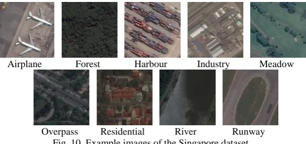
Singapore dataset is one of the recently introduced benchmark dataset for scene classification. This dataset consists of 1086 images with size of 256 × 256 pixels that represent nine scene categories. Example images of these categories are given in Fig. 10. The different classes in this dataset are unbalanced, the number of images in each class varies from 42 to 179.

3) Caltech 101 image dataset [34]

Caltech 101 dataset contains pictures of objects belonging to 101 categories plus one background category. The number of images in each class varies from 33 to 800 images per category. The size of each image is roughly 300×200 pixels. The examples of this dataset are presented in Fig. 11.

For this dataset, following the commonly used experimental protocol, we randomly pick out 30 images from each class as the training set in each numerical experiment conducted. We also leave the background category out due to the fact that the images inside this category are mostly unrelated.

Airplane Forest Harbour Industry Meadow

Overpass Residential River Runway

Fig. 10. Example images of the Singapore dataset

Ant Binocular Brain Cannon Ceiling fan Cup

Elephant Ferry Grand piano Hedgehog Leopards Mayfly

Nautilus Panda Revolver Schooner Stop sign Wheelchair

[image:18.595.145.455.70.216.2]

Fig.11. Example images of the Caltech 101 dataset

Table 11. Details of the benchmark image sets for numerical examples

Image Set Resolution Number of classes Number of samples Number of attributes

UCMerced 256×256×3 21 2100 4096

Singapore 256×256×3 9 1086 4096

Caltech 101 _{Roughly 300×200×3} 101 3030 4096

4.2. Experimental Setting

In the numerical experiments of this paper, for simplification, if no special declaration is made, the SSDRB classifier will not learn new classes, which means Algorithm 3 and Condition 4 are not used.

It is widely recognised that image labelling is a time-consuming task. In many real problems, one may only obtain the labels of a very small proportion of the existing images. The majority of them are unlabelled [17]. As a result, it is of great importance for the semi-supervised approaches to be able to effectively learn from the unlabelled images based on a small number of labelled ones. Therefore, in the numerical experiments of this paper, we limit the number of labelled images per class to be less than 10 and the total amount of the labelled ones to be less than 20% of the whole dataset.

We use the following well-known classification approaches for comparison: 1) SVM classifier [2];

2) KNN classifier [35];

classification results [36]–[39]. As the DRB classifier in this paper also involves a pre-trained DCNN as a feature descriptor, the two classifiers (SVM and KNN) are the most representative alternative approaches used for comparison. During the experiments, the value of

k

for KNN is set to be equal to L.

We also involve the state-of-the-art semi-supervised approaches for comparison: 3) Local and global consistency (LGC) based semi-supervised classifier [5];

4) Greedy gradient Max-Cut (GGMC) based semi-supervised classifier [8];

5) Laplacian SVM (LapSVM) classifier [40], [41];

6) AnchorGraphReg-based semi-supervised classifier with kernel weights (AnchorK) [42];

7) AnchorGraphReg-based semi-supervised classifier with LAE weights (AnchorL) [42].

There are also other well-known SVM- or graph-based semi-supervised approaches, i.e. Transductive SVM (TSVM) [13], TSVM [6] and Gaussian fields and harmonic functions based approaches [4]. However, previous work showed that the LapSVM, LGC, GGMC and GGMC are, in general, able to produce more accurate classification results [8]. Therefore, we only limit the comparison to only the seven algorithms listed above.

The free parameter  of the LGC classifier is set to be 0.99 as suggested in [5]. The free parameter  of the GGMC classifier is set to be



0.01 as suggested in [8]. LGC and GGMC use the KNN graph with kL . The LapSVM classifier uses the “one-versus-all” strategy for all the benchmark problems; the radial basis function kernel with  10 is used; the two free parameters _I and _A are set to be 1and 106, respectively; the number of neighbour,

k

, for computing the graph Laplacian is set to be 15 as suggested in [40]. The free parameter of AnchorK and AnchorL classifiers, s (number of the closest anchors) is set to be s3; for the AnchorL classifier, its iteration number of LAE is set to be 10 as suggested in [42].

We have to stress that during the experiments, all the comparative approaches involved are trained with same feature vectors extracted from the same, both labelled and unlabelled training images by the SSDRB classifier. It is also necessary to stress that without special declaration, all the reported results in this section are the average results after 50 Monte Carlo experiments by randomly picking out the labelled and unlabelled training images under the fixed ratios from the benchmark datasets. No out-of-sample classification is conducted, and all the unlabelled training images are used during the semi-supervised learning process.

4.3. Demonstration of the Proposed Approach

In this section, we will conduct a series of numerical experiments with the proposed SSDRB classifier based on the UCMerced dataset.

4.3.1. Influence of  on the performance of SSDRB classifier

[image:20.595.112.484.85.213.2]

Table 12. Performance of the SSDRB classifier with different values of 

φ 1.05 1.10 1.15 1.20 1.25 1.3

FSL a E

c

0.2430

Nd 161.1

Offline SSL b E 0.2194 0.2141 0.2159 0.2221 0.2258 0.2332

N 1637 1402.8 1194.9 1015.8 874.7 759.1

Online SSL-SBS e

E 0.2502 0.2365 0.2334 0.2345 0.2376 0.2396 N 1432.6 1192.8 1008.2 862.8 746.2 648.9 Online

SSL-CBC f

E 0.2287 0.2229 0.2237 0.2307 0.2335 0.2376 N 1581.6 1337.8 1127.7 960.1 825.1 712.6 a

Fully supervised learning (FSL); b Semi-supervised learning (SSL); c Error rate (E); d

[image:20.595.192.393.260.393.2]

Number of prototypes (N);e Sample-by-sample (SBS); f Chunk-by-chunk (CBC).

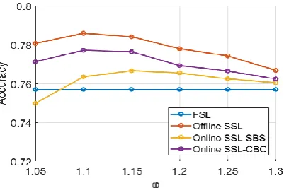
Fig. 12. The average accuracy curve of the SSDRB classifier

As one can see from Table 12 and Fig. 12, the higher the value of φ is, the less prototypes the SSDRB classifier identified during the semi-supervised learning process, and, thus, the system structure is less complex and the computational efficiency is higher. However, at the same time, it is obvious that the accuracy of the classification results is not linearly correlated with the value of φ. There is a certain range of φ values for the SSDRB classifier to achieve the best accuracy. Trading off the overall performance and system complexity, the best range of φ values for the experiments performed is



1.1;1.2



. For consistence, we use φ=1.2 in the rest of the

numerical examples in this section. However, one can also set different value for φ.

4.3.2. Influence of Lon the performance of the SSDRB classifier

In this numerical example, we randomly pick out L 1, 2, 3, …, 10 images from each class of the UCMerced dataset as the labelled training images and use the rest as the unlabelled ones to train the SSDRB classifier in both offline and online scenarios. Similar to the previous experiment, the semi-supervised learning is conducted on both sample-by-sample basis and chunk-by-chunk basis in the online scenario. The classification error rates of the SSDRB classifier on the unlabelled training set are reported in Table 13. The corresponding accuracy of the DRB classifier with different number of labelled images is depicted in Fig. 13.

[image:21.595.145.449.88.229.2]

Table 13. Performance of the SSDRB classifier with different number of labelled training samples Error Rates

L a 1 2 3 4 5

FSL 0.4568 0.3838 0.3439 0.3079 0.2903 Offline SSL 0.4270 0.3522 0.3082 0.2810 0.2612 Online SSL-SBS 0.4861 0.3914 0.3354 0.3002 0.2814 Online SSL-CBC 0.4401 0.3639 0.3203 0.2893 0.2718

L 6 7 8 9 10

FSL 0.2687 0.2575 0.2430 0.2346 0.2252 Offline SSL 0.2425 0.2333 0.2221 0.2157 0.2049 Online SSL-SBS 0.2622 0.2485 0.2345 0.2277 0.2184 Online SSL-CBC 0.2522 0.2418 0.2307 0.2205 0.2115 a _{Number of labelled training samples per class (L)}

Fig. 13. The accuracy of the SSDRB classifier with different number of labelled images

4.3.3. Influence of  on the active learning mechanism and performance of the SSDRB classifier

In the following numerical example, we investigate the influence of  on the active learning mechanism and the performance of the proposed SSDRB classifier. During the experiment, the value of  varies from 0.4 to 0.65 with the interval of 0.05. We randomly select 20 out of the 21 classes from the UCMerced dataset and pick out L10 images from each of them as the labelled training images. The rest are used as the unlabelled ones to train the SSDRB classifier in both offline and online scenarios. Similar to the previous experiment, the semi-supervised learning is conducted on both sample-by-sample basis and chunk-by-chunk basis in the online scenario. In order to count classification errors, for each newly gained class/fuzzy rule, we use the class labels of its dominant members as the label of this class/fuzzy rule. The classification error rates of the SSDRB classifier on the unlabelled training set are reported in Table 14. The numbers of classes after the training process during the experiment are also listed in the same table. The corresponding accuracy of the SSDRB classifier with different number of labelled images is depicted in Fig. 14.

[image:21.595.192.393.266.398.2]

[image:22.595.112.483.105.220.2]

Table 14. Performance of the SSDRB classifier with different values of γ

γ 0.4 0.45 0.5 0.55 0.6 0.65

FSL E 0.2604

F a 20

Offline SSL E 0.2549 0.2558 0.2388 0.2093 0.1663 0.1261

F 20.2 32.7 74.8 167.6 292.2 434.3

Online SSL-SBS E 0.2386 0.2215 0.1905 0.1461 0.0939 0.0469

F 25.2 55.3 141.6 304.8 523.1 758.9

Online SSL-CBC E 0.2812 0.2724 0.2527 0.2174 0.1710 0.1262

F 21.3 38.6 94.3 212.4 368.9 545.0

a

[image:22.595.202.403.260.417.2]

Number of fuzzy rules after training.

Fig. 14. The average accuracy of the SSDRB classifier with different values of γ

4.3.4. Performance of the SSDRB classifier on out-of-sample classification

Using the same experimental protocol as the previous experiment, we use the UCMerced dataset and randomly pick out L 10 images from each class as the labelled training images and use the rest as the unlabelled ones. However, in this numerical example, we randomly leave Q 5, 10, 15, 20, 25, 30 unlabelled images per class out to conduct the out-of-sample classification. Namely, the SSDRB classifier is trained in both offline and online scenarios based on L labelled and ( 100 L Q) unlabelled training images per class. After the training process is finished, the SSDRB classifier will conduct out-of-sample classification on the remainders without updating the system. The classification error rates of the SSDRB classifier on the out-of-sample classification are reported in Table 15. The corresponding accuracy of the SSDRB classifier with different number of labelled images is depicted in Fig. 15.

Table 15. Performance of the SSDRB classifier on out-of-sample classification Error Rate

Q a 5 10 15 20 25 30

FSL 0.2320 0.2319 0.2305 0.2300 0.2306 0.2292 Offline SSL 0.2078 0.2086 0.2104 0.2114 0.2124 0.2122 Online SSL-SBS 0.2183 0.2184 0.2192 0.2182 0.2190 0.2167 Online SSL-CBC 0.2141 0.2124 0.2135 0.2139 0.2163 0.2155 a _{Number of unlabelled samples per class for out-of-sample classification.}

[image:22.595.126.468.627.710.2]

[image:23.595.192.392.95.229.2]

Fig. 15. The accuracy of the SSDRB classifier on out-of-sample classification

4.4. Performance Comparison

In this subsection, we compare the performance of the proposed semi-supervised DRB (SSDRB) classifier with the seven state-of-the-art approaches based on the three benchmark problems listed in subsection 4.1. For a fair comparison, we only consider the performance of the SSDRB classifier applying offline semi-supervised learning. Therefore, all the numerical examples presented in this subsection are conducted in an offline scenario.

4.4.1. Numerical examples on UCMerced dataset

For the UCMerced dataset, we randomly pick out L 1, 2, 3, …, 10 images from each class as the labelled training images and use the rest as the unlabelled ones. The classification results of the SSDRB classifier and the seven comparative approaches are tabulated in Table 16 (the best results are bolded) in terms of the classification error rate on unlabelled training images.

Table 16. Performance comparison (UCM dataset) Error Rate

L 1 2 3 4 5

SSDRB 0.4270 0.3522 0.3082 0.2810 0.2612

SVM 0.6361 0.4907 0.4128 0.3667 0.3259

KNN 0.5708 0.5640 0.5279 0.4858 0.4675

LGC 0.8882 0.4321 0.3407 0.3075 0.2959

GGMC 0.8877 0.5019 0.4073 0.3833 0.3517

LapSVM 0.7547 0.5588 0.4731 0.4137 0.3682

AnchorK 0.4563 0.4068 0.3621 0.3474 0.3323

AnchorL 0.4212 0.3638 0.3259 0.3162 0.2984

L 6 7 8 9 10

SSDRB 0.2425 0.2333 0.2221 0.2157 0.2049

SVM 0.2895 0.2701 0.2548 0.2370 0.2198

KNN 0.4508 0.4381 0.4285 0.4254 0.4132

LGC 0.2820 0.2829 0.2820 0.2814 0.2825

GGMC 0.3417 0.3321 0.3419 0.3435 0.3397

LapSVM 0.3322 0.3047 0.2788 0.2558 0.2403

AnchorK 0.3201 0.3119 0.2981 0.2894 0.2827

[image:23.595.130.468.460.697.2]

[image:24.595.202.404.81.211.2]

Fig. 16. Accuracy comparison (UCM dataset)

4.4.2. Numerical examples on Singapore dataset

For the Singapore dataset, we randomly choose L 1, 2, 3, …, 10 images from each class as the labelled training images and use the rest as unlabelled one to train the SSDRB classifier in an offline scenario. We compare its performance with the seven algorithms listed above. The average classification error rates on the (1086-9L) unlabelled training images are tabulated in Table 17 (the best results are bolded). The corresponding accuracy curves are presented in Fig. 17.

Table 17. Performance comparison (Singapore dataset) Error Rate

L 1 2 3 4 5

SSDRB 0.2199 0.1232 0.0803 0.0767 0.0660

SVM 0.4370 0.2948 0.2208 0.1827 0.1562

KNN 0.3743 0.4049 0.3124 0.3247 0.2685

LGC 0.9142 0.2306 0.1258 0.1023 0.0780

GGMC 0.9139 0.2885 0.2288 0.2327 0.1761

LapSVM 0.7465 0.4966 0.3804 0.3391 0.2768

AnchorK 0.2234 0.1730 0.1556 0.1500 0.1377

AnchorL 0.2107 0.1580 0.1381 0.1268 0.1180

L 6 7 8 9 10

SSDRB 0.0601 0.0548 0.0473 0.0488 0.0465

SVM 0.1337 0.1179 0.1066 0.1126 0.0936

KNN 0.2797 0.2541 0.2567 0.2470 0.2328

LGC 0.0814 0.0823 0.0848 0.0840 0.0922

GGMC 0.1812 0.1924 0.2147 0.2033 0.1734

LapSVM 0.2510 0.2175 0.1842 0.1655 0.1479

AnchorK 0.1374 0.1280 0.1335 0.1298 0.1225

[image:24.595.132.467.362.604.2]

[image:25.595.202.404.81.211.2]

Fig. 17. Accuracy comparison (Singapore dataset)

4.4.3. Numerical examples on Caltech 101 dataset

[image:25.595.159.431.357.650.2]

For Caltech 101 dataset, due to the fact that each class has only 30 images , we randomly choose L 1, 2, 3, 4, 5 images from each class as labelled training images and use the rest as unlabelled one to train the SSDRB classifier in an offline scenario. Then, we compare its performance with the seven algorithms and report the classification error rates on the (3030-101L) unlabelled training images in Table 18 (the best results are bolded). We also present the average accuracy curves in Fig. 18.

Table 18. Performance comparison (Caltech 101 dataset) Error Rate

L 1 2 3 4 5

SSDRB 0.3941 0.3173 0.2780 0.2588 0.2472 SVM 0.6707 0.5215 0.4494 0.3941 0.3602 KNN 0.9092 0.8236 0.8358 0.8077 0.7867 LGC 0.7699 0.3566 0.3032 0.2810 0.2708 GGMC 0.7716 0.3788 0.3132 0.2921 0.2836 LapSVM 0.5198 0.3636 0.3149 0.2891 0.2725 AnchorK 0.6203 0.5382 0.4580 0.4045 0.3724 AnchorL 0.5398 0.4626 0.4010 0.3730 0.3445

Fig. 18. Accuracy comparison (Caltech 101 dataset)

4.5. Discussions

From Tables 16-18 and Figs. 16-18 one can see that, the SSDRB classifier is able to provide highly accurate classification results with only a very small number of labelled training images. It consistently outperforms all the seven comparative classification algorithms (both the most widely used ones and the “state-of-the-art” semi-supervised ones) in all the three popular benchmarks in the field of computer vison.

[image:25.595.204.404.516.646.2]

1) supports online training;

2) learns new classes actively, and

3) classifies out-of-sample images.

These are also demonstrated on the numerical examples in this section. In addition, due to its “one pass” type learning process (there is no error propagation during the process), the SSDRB classifier has a very high tolerance to the incorrectly pseudo-labelled images, and thus, its performance is very high in complex problems even with very small amount of labelled training images.

5. Conclusion

In this paper, we propose a semi-supervised deep rule-based (SSDRB) classifier. It offers very high classification rates on the unlabelled images surpassing other methods and, at same time, a human interpretable set of IF…THEN… rules after a highly transparent semi-supervised learning process. Compared with the existing semi-supervised learning approaches, the proposed SSDRB classifier has the following distinctive features:

1) it has a prototype-based nature;

2) it is able to learn from online image stream (video);

3) its system structure is human interpretable;

4) it is able to perform classification on out-of-sample images.

Numerical examples based on large-scale benchmark image sets demonstrate the strong performance of the SSDRB classifier introduced in this paper and also show its distinctive features.

As future work, we will develop more effective semi-supervised learning strategies for the SSDRB classifier in online scenarios. We will also investigate the optimality of the proposed approach.

Reference

[1] A. M. Kaplan and M. Haenlein, “Users of the world, unite! The challenges and opportunities of Social Media,” Bus. Horiz., vol. 53, no. 1, pp. 59–68, 2010.

[2] N. Cristianini and J. Shawe-Taylor, An introduction to support vector machines and other kernel-based learning methods. Cambridge: Cambridge University Press, 2000.

[3] C. M. Bishop, Pattern recognition and machine learning. New York: Springer, 2006.

[4] X. Zhu, Z. Ghahraman, and J. D. Lafferty, “Semi-supervised learning using gaussian fields and harmonic functions,” in International conference on Machine learning, 2003, pp. 912–919.

[5] D. Zhou, O. Bousquet, T. N. Lal, J. Weston, and B. Schölkopf, “Learning with local and global consistency,” in Adv. Neural. Inform. Process Syst, 2004, pp. 321–328.

[6] O. Chapelle and A. Zien, “Semi-supervised classification by low density separation,” in AISTATS, 2005, pp. 57–64.

[7] M. Guillaumin, J. J. Verbeek, and C. Schmid, “Multimodal semi-supervised learning for image classification,” in IEEE Conference on Computer Vision & Pattern Recognition, 2010, pp. 902–909. [8] J. Wang, T. Jebara, and S. F. Chang, “Semi-supervised learning using greedy Max-Cut,” J. Mach.

Learn. Res., vol. 14, pp. 771–800, 2013.

[9] A. Iwayemi and C. Zhou, “SARAA: Semi-Supervised Learning for Automated Residential Appliance Annotation,” IEEE Trans. Smart Grid, vol. 8, no. 2, p. 779, 2017.

[10] F. Wang, C. Zhang, H. C. Shen, and J. Wang, “Semi-supervised classification using linear neighborhood propagation,” in IEEE Conference on Computer Vision & Pattern Recognition, 2006, pp. 160–167. [11] S. Xiang, F. Nie, and C. Zhang, “Semi-supervised classification via local spline regression,” IEEE

Trans. Pattern Anal. Mach. Intell., vol. 32, no. 11, pp. 2039–2053, 2010.