THE ZIG-ZAG PROCESS AND SUPER-EFFICIENT SAMPLING FOR BAYESIAN ANALYSIS OF BIG DATA
By Joris Bierkens∗, Paul Fearnhead∗ and Gareth Roberts∗
Delft University of Technology, Lancaster University and University of Warwick
Abstract Standard MCMC methods can scale poorly to big data settings due to the need to evaluate the likelihood at each iteration. There have been a number of approximate MCMC algorithms that use sub-sampling ideas to reduce this computational burden, but with the drawback that these algorithms no longer target the true poste-rior distribution. We introduce a new family of Monte Carlo meth-ods based upon a multi-dimensional version of the Zig-Zag process of Bierkens and Roberts(2017), a continuous time piecewise determinis-tic Markov process. While traditional MCMC methods are reversible by construction (a property which is known to inhibit rapid conver-gence) the Zig-Zag process offers a flexible non-reversible alternative which we observe to often have favourable convergence properties. We show how the Zig-Zag process can be simulated without discretisation error, and give conditions for the process to be ergodic. Most impor-tantly, we introduce a sub-sampling version of the Zig-Zag process that is an example of anexact approximate scheme, i.e. the resulting approximate process still has the posterior as its stationary distri-bution. Furthermore, if we use a control-variate idea to reduce the variance of our unbiased estimator, then the Zig-Zag process can be super-efficient: after an initial pre-processing step, essentially inde-pendent samples from the posterior distribution are obtained at a computational cost which does not depend on the size of the data.
1. Introduction. The importance of Markov chain Monte Carlo tech-niques in Bayesian inference shows no signs of diminishing. However, all commonly used methods are variants on the Metropolis-Hastings (MH) algo-rithm (Metropolis et al.,1953;Hastings,1970) and rely on innovations which date back over 60 years. All MH algorithms simulate realisations from a dis-crete reversible ergodic Markov chain with invariant distribution π which is (or is closely related to) the target distribution, i.e. the posterior distri-bution in a Bayesian context. The MH algorithm gives a beautifully simple
∗
The authors acknowledge the EPSRC for support under grants EP/D002060/1 (CRiSM) and EP/K014463/1 (iLike).
MSC 2010 subject classifications:Primary 65C60; secondary 65C05, 62F15, 60J25
Keywords and phrases:MCMC, non-reversible Markov process, piecewise deterministic Markov process, Stochastic Gradient Langevin Dynamics, sub-sampling, exact sampling
though flexible recipe for constructing such Markov chains, requiring only local information aboutπ(typically pointwise evaluations ofπand, perhaps, its derivative at the current and proposed new locations) to complete each iteration.
However new complex modelling and data paradigms are seriously chal-lenging these established methodologies. Firstly, the restriction of traditional MCMC to reversible Markov chains is a serious limitation. It is now well-understood both theoretically (Hwang, Hwang-Ma and Sheu, 1993; Chen and Hwang,2013; Rey-Bellet and Spiliopoulos,2015;Bierkens,2015; Dun-can, Leli`evre and Pavliotis, 2016) and heuristically (Neal, 1998) that non-reversible chains offer potentially massive advantages over non-reversible counter-parts. The need to escape reversibility, and create momentum to aid mixing throughout the state space is certainly well-known, and motivates a num-ber of modern MCMC methods, including the popular Hamiltonian MCMC (Duane et al.,1987).
A second major obstacle to the application of MCMC for Bayesian in-ference is the need to process potentially massive data-sets. Since MH al-gorithms in their pure form require a likelihood evaluation – and thus pro-cessing the full data-set – at every iteration, it can be impractical to carry out large numbers of MH iterations. This has led to a range of alterna-tives that use sub-samples of the data at each iteration (Welling and Teh,
2011;Maclaurin and Adams,2014;Ma, Chen and Fox,2015;Quiroz, Villani and Kohn, 2015), or that partition the data into shards, run MCMC on each shard, and then attempt to combine the information from these dif-ferent MCMC runs (Neiswanger, Wang and Xing, 2013;Scott et al.,2016;
Wang and Dunson, 2013; Li, Srivastava and Dunson,2017). However most of these methods introduce some form of approximation error, so that the final sample will be drawn from some approximation to the posterior, and the quality of the approximation can be impossible to evaluate. As an ex-ception the Firefly algorithm (Maclaurin and Adams, 2014) samples from the exact distribution of interest (but see the comment below).
distribution. Furthermore, if we also use control variate ideas to reduce the variance of our sub-sampling estimator of the gradient, the resulting Zig-Zag with Control Variates (ZZ-CV) algorithm has remarkablesuper-efficient scaling properties for large data sets.
We will call an algorithm super-efficient if it is able to generate inde-pendent samples from the target distribution at a higher efficiency than if we would draw independently from the target distribution at the cost of evaluating all data. The only situation we are aware of where we can im-plement super-efficient sampling is with simple conjugate models, where the likelihood function has a low-dimensional summary statistic which can be evaluated at costO(n), where n is the number of observations, after which we can obtain independent samples from the posterior distribution at a cost of O(1) by using the functional form of the posterior distribution. The ZZ-CV can replicate this computational efficiency: after a pre-computation of
O(n), we are able to obtain independent samples at a cost ofO(1). In this sense it contrasts with the Firefly algorithm (Maclaurin and Adams, 2014) which has an ESS per datum which decreases approximately as 1/n where
nis the size of the data, so that the gains of this algorithm do not increase withn; see (Bouchard-Cˆot´e, Vollmer and Doucet,2015, Section 4.6).
This breakthrough is based upon the Zig-Zag process, a continuous time piecewise deterministic Markov process (PDMP). Given a d-dimensional differentiable target density π, Zig-Zag is a continuous-time non-reversible stochastic process with continuous, piecewise linear trajectories on Rd. It moves with constant velocity, Θ∈ {−1,1}d, until one of the velocity
compo-nents switches sign. The event time and choice of which direction to reverse is controlled by a collection of state-dependent switching rates, (λi)di=1 which
in turn are constrained via an identity (2) which ensures that π is a sta-tionary distribution for the process. The process intrinsically is constructed in continuous-time, and it can be easily simulated using standard Poisson thinning arguments as we shall see in Section3.
The use of PDMPs such as the Zig-Zag processes is an exciting and mostly unexplored area in MCMC. The first occurrence of a PDMP for sampling purposes is in the computational physics literature (Peters and De With,2012), which in one dimension coincides with the Zig-Zag process. In
density function. As we will see in Section2.4, this difference has a beneficial effect on the ergodic properties of the Zig-Zag process. The one-dimensional Zig-Zag process is analysed in detail in e.g.Fontbona, Gu´erin and Malrieu
(2012);Monmarch´e (2014);Fontbona, Gu´erin and Malrieu(2016);Bierkens and Roberts(2017).
Since the first version of this paper was conceived already several other related theoretical and methodological papers have appeared. In particular we mention here results on exponential ergodicity of the BPS (Deligiannidis, Bouchard-Cˆot´e and Doucet,2017) and ergodicity of the multi-dimensional Zig-Zag process (Bierkens, Roberts and Zitt, 2017). The Zig-Zag process has the advantage that it is ergodic under very mild conditions, which in particular means that we are not required to choose a refreshment rate. At the same time, the BPS seems more ‘natural’, in that it tries to minimise the bounce rate and the change in direction at bounces, and it may be more efficient for this reason. However it is a challenge to make a direct comparison in efficiency of the two methods since the efficiency depends both on the computational effort per unit of continuous time of the respective algorithms, as well as the mixing time of the underlying processes. Therefore we expect analysing the relative efficiency of PDMP based algorithms to be an important area of continued research for years to come.
A continuous-time sequential Monte Carlo algorithm for scalable Bayesian inference with big data, the SCALE algorithm, is given in Pollock et al.
(2016). Advantages that Zig-Zag has over SCALE is that it avoids the issue of controlling the stability of importance weights, and it is simpler to imple-ment. Whereas the SCALE algorithm is well-adapted for the use of parallel architecture computing, and has particularly simple scaling properties for big data.
1.1. Notation. For a topological space X let B(X) denote the Borelσ -algebra. We write R+ := [0,∞). If h : Rd → R is differentiable then ∂ih
denotes the function ξ 7→ ∂h∂ξ(ξ)
i . We equip E := R
d× {−1,+1}d with the
product topology of the Euclidean topology onRdand the discrete topology on {−1,+1}d. Elements in E will often be denoted by (ξ, θ) with ξ ∈
Rd and θ ∈ {−1,+1}d. For g : E →
R differentiable in its first argument we will use∂igto denote the function (ξ, θ)7→ ∂g∂ξ(ξ,θi ),i= 1, . . . , d.
2. The Zig-Zag process. The Zig-Zag process is a continuous time Markov process whose trajectories lie in the spaceE=Rd× {−1,+1}dand will be denoted by (Ξ(t),Θ(t))t≥0. They can be described as follows: at
is linear with dtdΞ(t) = Θ(t). The rates at which the flips in Θ(t) occur are time inhomogeneous: thei-th component of Θ switches at rateλi(Ξ(t),Θ(t)),
whereλi:E →R+ fori= 1, . . . , d are continuous functions.
2.1. Construction. For a given (ξ, θ)∈E, we may construct a trajectory of (Ξ,Θ) of the Zig-Zag process with initial condition (ξ, θ) as follows.
• Let (T0,Ξ0,Θ0) := (0, ξ, θ). • Fork= 1,2, . . .
– Letξk(t) := Ξk−1+ Θk−1t,t≥0
– Fori= 1, . . . , d, let τik be distributed according to
P(τik≥t) = exp
−
Z t 0
λi(ξk(s),Θk−1) ds
.
– Leti0:= argmini∈{1,...,d}τik and letTk:=Tk−1+τik0.
– Let Ξk:=ξk(Tk). – Let
Θk(i) :=
Θk−1(i) ifi6=i0,
−Θk−1(i) ifi=i 0
This procedure defines a sequence ofskeleton points(Tk,Ξk,Θk)∞k=0inR+× E, which correspond to the time and position at which the direction of the process changes. The trajectoryξk(t) represents the position of the process at time Tk−1+t until timeTk, for 0≤t≤Tk−Tk−1. The time until the next skeleton event is characterized as the smallest time of a set of events in d simultaneous point processes, where each point process corresponds to switching of a different component of the velocity. For the i-th of these processes, events occur at rate λi(ξk(s),Θk−1), and τik is defined to be the
time to the first event for thei-th component. The component for which the earliest event occurs isi0. This defines τik0, the time between the (k−1)th andkth skeleton point, and the component,i0, of the velocity that switches. The piecewise deterministic trajectories (Ξ(t),Θ(t)) are now obtained as
(Ξ(t),Θ(t)) := (Ξk+ Θk(t−Tk),Θk) for t∈[Tk, Tk+1), k= 0,1,2, . . . .
The only step in this procedure which presents a computational challenge is the simulation of the random times (Tik) and a significant part of this paper will consider obtaining these in a numerically efficient way.
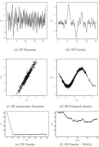
Figure1 displays trajectories of the Zig-Zag process for several examples of invariant distributions. The name of the process is derived by thezig-zag nature of paths that the process produces. Figure1shows an important dif-ference in the output of the Zig-Zag process, as compared to a discrete-time MCMC algorithm: the output of is a continuous-time sample path. The bot-tom row of plots in Figure1also gives a comparison to a reversible MCMC algorithm, Metropolis Adjusted Langevin (MALA Roberts and Tweedie,
1996), and demonstrates an advantage of a non-reversible sampler: it can cope better with a heavy tailed target. This is most easily seen if we start the process out in the tail, as in the figure. The velocity component of the Zig-Zag process enables it to quickly return to the mode of the distribution, whereas the reversible algorithm behaves like a random walk in the tails, and takes much longer to return to the mode.
2.2. Invariant distribution. The most important aspect of the Zig-Zag process is that in many cases the switching rates are directly related to an easily identifiable invariant distribution. Let C1(Rd) denote the space of continuously differentiable functions on Rd. For θ ∈ {−1,+1}d and i ∈ {1, . . . , d}, letFi[θ]∈ {−1,+1}d denote the binary vector obtained by
flip-ping thei-th component of θ; i.e.
(Fi[θ])j =
(
θj ifi6=j,
−θj ifi=j.
.
We introduce the following assumption.
Assumption 2.1. For some function Ψ∈C1(Rd) satisfying
(1)
Z
Rd
exp(−Ψ(ξ))dξ <∞
we have
(2) λi(ξ, θ)−λi(ξ, Fi[θ]) =θi∂iΨ(ξ) for all(ξ, θ)∈E, i= 1, . . . , d.
Throughout this paper we will refer to Ψ as thenegative log density. Let
µ0denote the measure onB(E) such that, forA∈ B(Rd) andθ∈ {−1,+1}d,
0 50 100 150 200
−3
−2
−1
0
1
2
3
t
Ξ
(
t
)
(a) 1D Gaussian
0 50 100 150 200
−5
0
5
10
t
Ξ
(
t
)
(b) 1D Cauchy
−2 −1 0 1 2
−2
−1
0
1
2
Ξ1(t)
Ξ2(
t
)
(c) 2D anisotropic Gaussian
−2 −1 0 1 2
−2
−1
0
1
2
Ξ1(t)
Ξ2(
t
)
(d) 2D S-shaped density
0 500 1000 1500 2000 2500 3000 3500
0
100
200
300
400
500
Time
Ξ1(
t
)
(e) 1D Cauchy
0 500 1000 1500 2000
0
100
200
300
400
500
Iteration
Ξ1(
t
)
[image:7.612.141.463.125.603.2](f) 1D Cauchy – MALA
Figure 1: Top two rows: example trajectories of the canonical Zig-Zag pro-cess. In (a) and (b) the horizontal axis shows time and the vertical axis the Ξ-coordinate of the 1D process. In (c) and (d), the trajectories inR2 of (Ξ1,Ξ2) are plotted. Bottom row: Zig-Zag process (e) and MALA (f) for a
Theorem 2.2. Suppose Assumption 2.1 holds. Let µ denote the
proba-bility distribution on E such thatµ has Radon-Nikodym derivative
(3) dµ
dµ0(ξ, θ) =
exp(−Ψ(ξ))
Z , (ξ, θ)∈E,
whereZ =REexp(−Ψ)dµ0. Then the Zig-Zag process(Ξ,Θ)with switching rates (λi)di=1 has invariant distribution µ.
The proof is located in the Section 1 of the Supplementary Material. We see that under the invariant distribution of the Zig-Zag process, ξ and θ
are independent, with ξ having density proportional to exp(−Ψ(ξ)) and θ
having a uniform distribution on the points in{−1,+1}d.
For a ∈ R, let (a)+ := max(0, a) and (a)− := max(0,−a) denote the positive and negative parts of a, respectively. We will often use the trivial identitya= (a)+−(a)−without comment. The following result characterizes the switching rates for which (2) holds.
Proposition 2.3. Suppose λ: E → Rd+ is continuous. Then
Assump-tion2.1is satisfied if and only if there exists a continuous function γ :E→ Rd+ such that for all i= 1, . . . , d and (ξ, θ) ∈E, γi(ξ, θ) = γi(ξ, Fi[θ]) and,
for Ψ∈C1(Rd) satisfying (1),
(4) λi(ξ, θ) = (θi∂iΨ(ξ))++γi(ξ, θ).
The proof is located in Section 1 of the Supplementary Material.
2.3. Zig-Zag process for Bayesian inference. One application of the Zig-Zag process is as an alternative to MCMC for sampling from posterior dis-tributions in Bayesian statistics. We show here that it is straightforward to derive a class of Zig-Zag processes that have a given posterior distribution as their invariant distribution. The dynamics of the Zig-Zag process only de-pend on knowing the posterior density up to a constant of proportionality.
To keep notation consistent with that used for the Zig-Zag process, let
ξ ∈ Rd denote a vector of continuous parameters. We are given a prior
density function for ξ, which we denote by π0(ξ), and observations x1:n =
(x1, . . . , xn). Our model for the data defines a likelihood functionL(x1:n|ξ).
Thus the posterior density function is
π(ξ)∝π0(ξ)L(x1:n|ξ).
We can writeπ(ξ) in the form of the previous section,
π(ξ) = 1
Z exp(−Ψ(ξ)), ξ ∈R
where Ψ(ξ) =−logπ0(ξ)−logL(x1:n|ξ), andZ =R
Rdexp(−Ψ(ξ))dξ is the unknown normalising constant. Now assuming that logπ0(ξ) and logL(x1:n|ξ)
are both continuously differentiable with respect to ξ, from (4) a Zig-Zag process with rates
λi(ξ, θ) = (θi∂iΨ(ξ))+
will have the posterior densityπ(ξ) as the marginal of its invariant distribu-tion. We call the process with these rates theCanonical Zig-Zag process for the negative log density Ψ. As explained in Proposition2.3, we can construct a family of Zig-Zag processes with the same invariant distribution by choos-ing any set of functions γi(ξ, θ), for i = 1, . . . , d, which take non-negative
values and for whichγi(ξ, θ) =γi(ξ, Fi[θ]), and setting
λi(ξ, θ) = (θi∂iΨ(ξ))++γi(ξ, θ), fori= 1, . . . , d.
The intuition here is that λi(ξ, θ) is the rate at which we transition from θ
toFi[θ]. The conditionγi(ξ, θ) =γi(ξ, Fi[θ]) means that we increase by the
same amount both the rate at which we will transition from θ toFi[θ] and
vice versa. As our invariant distribution places the same probability of being in a state with velocityθas that of being in stateFi[θ], these two changes in
rate cancel out in terms of their effect on the invariant distribution. Changing the rates in this way does impact the dynamics of the process, with largerγi
values corresponding to more frequent changes in the velocity of the Zig-Zag process, and we would expect the resulting process to mix more slowly.
Under the assumption that the Zig-Zag process has the desired invariant distribution and is ergodic, it follows from the Birkhoff ergodic theorem that for any bounded continuous functionf :E→R,
lim
t→∞
1
t Z t
0
f(Ξ(s),Θ(s))ds=
Z
E
f dµ,
for any initial condition (ξ, θ) ∈E. Sufficient conditions for ergodicity will be discussed in the following section. Takingγ to be positive and bounded everywhere ensures ergodicity, as will be established in Theorem2.10.
2.4. Ergodicity of the Zig-Zag process. We have established in Section2.2
that for any continuously differentiable, positive density π on Rda Zig-Zag process can be constructed that hasπ as its marginal stationary density. In order for ergodic averagesT1 RT
0 f(Ξ(s))dsof the Zig-Zag process to converge
asymptotically toπ(f), we further require (Ξ(t),Θ(t)) to be ergodic, i.e. to admit a unique invariant distribution.
each invariant for the process (Ξ(t),Θ(t)). For the one-dimensional Zig-Zag process, (exponential) ergodicity has already been established under mild conditions (Bierkens and Roberts,2017). As we discuss below, irreducibility, and thus ergodicity, can be established for large classes of multi-dimensional target distributions, such as i.i.d. Gaussian distributions, and also if the switching ratesλi(ξ, θ) are positive for all i= 1, . . . , d, and (ξ, θ)∈E.
LetPt((ξ, θ),·) be the transition kernel of the Zig-Zag process with initial condition (ξ, θ). A functionf :E→Ris callednorm-likeif limkξk→∞f(ξ, θ) =
∞for all θ∈ {−1,+1}d. Letk · k
TV denote the total variation norm on the
space of signed measures. First we consider the one-dimensional case.
Assumption 2.4. Suppose d= 1 and there existsξ0>0 such that
(i) infξ≥ξ0λ(ξ,+1)>supξ≥ξ0λ(ξ,−1), and
(ii) infξ≤−ξ0λ(ξ,−1)>supξ≤−ξ0λ(ξ,+1).
Proposition 2.5. (Bierkens and Roberts, 2017, Theorem 5) Suppose
Assumption2.4 holds. Then there exists a function f :E →[1,∞) which is norm-like such that the Zig-Zag process isf-exponentially ergodic, i.e. there exists a constant κ >0 and 0< ρ <1 such that
kPt((ξ, θ),·)−πkTV≤κf(ξ, θ)ρt for all (ξ, θ)∈E andt≥0.
Example 2.6. As an example of fundamental importance, which will
also be used in the proof of Theorem2.10, consider a one-dimensional Gaus-sian distribution. For simplicity letπ(ξ) be centred,π(ξ) = √1
2πσ2 exp
−2ξσ22
for someσ >0. According to (4) the switching rates take the form
λ(ξ, θ) = θξ/σ2++γ(ξ), (ξ, θ)∈E.
As long asγis bounded from above, Assumption2.4is satisfied. In particular this holds ifγ is equal to a non-negative constant.
Remark2.7. We say a probability density functionπ is ofproduct form
ifπ(ξ) =Qd
i=1πi(ξi), whereπi :Rd→(0,∞) are one-dimensional probabil-ity densprobabil-ity functions. When its target densprobabil-ity is of product form the Zig-Zag process is the concatenation of independent Zig-Zag processes. In this case the negative log density is of the form Ψ(ξ) =Pd
i=1Ψi(ξi) and the switching
rate for the i-th component of θis
(5) λi(ξ, θ) = θiΨ0i(ξi)
+
As long asγi(ξ) =γi(ξi), i.e. ifγi(ξ) only depends on thei-th coordinate ofξ,
the switching rate of coordinateiis independent of the other coordinatesξj,
j6=i. It follows that the switches of thei-th coordinate can be generated by a one-dimensional time inhomogeneous Poisson process, which is independent of the switches in the other coordinates. As a consequence thed-dimensional Zig-Zag process (Ξ(t),Θ(t)) = (Ξ1(t), . . . ,Ξ
d(t),Θ1(t), . . . ,Θd(t)) consists of
a combination ofdindependent Zig-Zag processes (Ξi(t),Θi(t)),i= 1, . . . , d.
Suppose P(x, dy) is the transition kernel of a Markov chain on a state space E. We say that the Markov chain associated to P is mixing if there exists a probability distributionπ on E such that
lim
k→∞kP
k(x,·)−πk
TV= 0 for all x∈E.
For any continuous time Markov process with family of transition kernels
Pt(x, dy) we can consider the associatedtime-discretized process, which is a Markov chain with transition kernelQ(x, dy) :=Pδ(x, dy) for a fixedδ >0. The value ofδ will be of no significance in our use of this construction.
Proposition 2.8. Suppose π is of product form and λ : E → Rd+
ad-mits the representation (5) with γi(ξ) only depending on {ξi, i = 1, . . . , d}.
Furthermore suppose that for every i= 1, . . . , d, the one-dimensional time-discretized Zig-Zag process corresponding to switching rate λi is mixing in
R× {−1,+1}. Then the time-discretized d-dimensional Zig-Zag process with switching rates(λi) is mixing. In particular, the multi-dimensional Zig-Zag
process admits a unique invariant distribution.
Proof. This follows from the decomposition of the d-dimensional
Zig-Zag process asd one-dimensional Zig-Zag processes and Lemma 1.1 in the Supplementary material.
Example 2.9. Continuing Example 2.6, consider the simple case in
which π is of product form with eachπi a centered Gaussian density
func-tion with varianceσ2
i. It follows from Proposition2.8and Example2.6that
the multi-dimensional canonical Zig-Zag process (i.e. the Zig-Zag process withγi ≡0) is mixing. This is different from the Bouncy Particle Sampler
(Bouchard-Cˆot´e, Vollmer and Doucet, 2015), which is not ergodic for an i.i.d. Gaussian without ‘refreshments’ of the momentum variable.
Theorem 2.10. Suppose λ:E → (0,∞)d, in particularλi(ξ, θ) is
pos-itive for all i = 1, . . . , d and (ξ, θ) ∈E. Then there exists at most a single invariant measure for the Zig-Zag process with switching rateλ.
The proof of this result consists of a Girsanov change of measure with respect to a Zig-Zag process targeting an i.i.d. standard normal distribution, which we know to be irreducible. The irreducibility then carries over to the Zig-Zag process with the stated switching rates. A detailed proof can be found in the Supplementary material.
Remark2.11. Based on numerous experiments, we conjecture that the
canonical multi-dimensional Zig-Zag process is ergodic in general under only mild conditions. A detailed investigation of ergodicity will be the subject of a forthcoming paper (Bierkens, Roberts and Zitt,2017).
3. Implementation. As mentioned earlier, the main computational challenge is an efficient simulation of the random times Tik introduced in Section2.1. We will focus on simulation by means of Poisson thinning.
Proposition3.1 (Poisson thinning,Lewis and Shedler(1979)). Letm:
R+ → R+ and M : R+ → R+ be continuous such that m(t) ≤ M(t) for t≥0. Letτ1, τ2, . . . be the increasing finite or infinite sequence of points of a Poisson process with rate function (M(t))t≥0. For all i, delete the point τi with probability 1−m(τi)/M(τi). Then the remaining points, τe
1, e τ2, . . .
say, form a non-homogeneous Poisson process with rate function(m(t))t≥0.
Now for a given initial point (ξ, θ) ∈ E, let mi(t) := λi(ξ +θt, θ), for
i= 1, . . . , d, and suppose we have available continuous functions Mi(t) such
that mi(t) ≤Mi(t) for i= 1, . . . , d and t ≥0. We call these (Mi)di=1
com-putational bounds for (mi)di=1. We can use Proposition 3.1 to obtain the
first switching times (τe 1
i)di=1 from a (theoretically infinite) collection of
pro-posed switching times (τi1, τi2, . . .)di=1 given the initial point (ξ, θ), and use the obtained skeleton point at time eτ1 := mini∈{1,...,d}eτ
1
i as a new initial
point (which is allowed by the strong Markov property) with the compo-nent i0 = argmini∈{1,...,d}eτ
1
i of θswitched.
The strong Markov property of the Zig-Zag process simplifies the compu-tational procedure further: we can draw for each componenti= 1, . . . , dthe first proposed switching timeτi:=τi1, determinei0 := argmini∈{1,...,d}τiand
decide whether the appropriate component ofθis switched at this time with probability mi0(τ)/Mi0(τ), whereτ := τi0. Then since τ is a stopping time
at time τ as new starting point, regardless of whether we switch a compo-nent ofθat the obtained skeleton point. A full computational procedure for simulating the Zig-Zag process is given by Algorithm1.
Algorithm 1:Zig-Zag Sampling (ZZ) Input: initial condition (ξ, θ)∈E.
Output: a sequence of skeleton points (Tk,Ξk,Θk)∞
k=0.
1. (T0,Ξ0,Θ0) := (0, ξ, θ).
2. fork= 1,2, . . .
(a) Definemi(t) :=λi(Ξk−1+ Θk−1t,Θk−1) fort≥0 andi= 1, . . . , d.
(b) Fori= 1, . . . , d, let (Mi) denote computational bounds for (mi).
(c) Drawτ1, . . . , τdsuch thatP(τi≥t) = exp
−Rt
0Mi(s)ds
.
(d) i0:= argmini=1,...,d{τi}andτ:=τi0.
(e) (Tk,Ξk) := (Tk−1+τ,Ξk−1+ Θk−1τ)
(f) With probabilitymi0(τ)/Mi0(τ),
• Θk:=Fi0[Θ
k−1
],
otherwise
• Θk:= Θk−1.
3.1. Computational bounds. We now come to the important issue of ob-taining computational bounds for the Zig-Zag Process, i.e. useful upper bounds for the switching rates (mi). If we can compute the inverse function
Gi(y) := inf{t ≥ 0 : Hi(t) ≥ y} of Hi :t 7→
Rt
0Mi(s) ds, we can simulate τ1, . . . , τd using the CDF inversion technique, i.e. by drawing i.i.d. uniform
random variables U1, . . . , Ud and setting τi:=Gi(−logUi), i= 1, . . . d.
Let us ignore the subscript ifor a moment. Examples of computational bounds are piecewise affine bounds of the form M : t 7→ (a+bt)+, with
a, b∈R, and the constant bounds M :t7→c forc≥0. It is also possible to simulate using the combined rateM :t7→min(c,(a+bt)+). In these cases,
H(t) = Rt
0M(s) ds is piecewise linear or quadratic and non-decreasing, so
we can obtain an explicit expression for the inverse function,G.
state space before a new evaluation of a component ofλis required, and we will pay close attention to the scaling of Mi with respect to the number of
available observations in a Bayesian inference setting.
3.2. Example: globally bounded log density gradient. If there are con-stants ci > 0 such that supξ∈Rd|∂iΨ(ξ)| ≤ ci, i= 1, . . . d, then we can use the global upper boundsMi(t) =ci fort≥0. Indeed, for (ξ, θ)∈E,
λi(ξ, θ) = (θi∂iΨ(ξ))+≤ |∂iΨ(ξ)| ≤ci.
Algorithm1 may be used withMi ≡ci fori= 1, . . . , d at every iteration.
This situation arises with heavy-tailed distributions. E.g. ifπ is Cauchy,
then Ψ(ξ) = log(1 +ξ2), and consequentlyλ(ξ, θ) =1+2θξξ2
+
≤1.
3.3. Example: negative log density with dominated Hessian. Another im-portant case is when there exists a positive definite matrixQ∈Rd×dwhich dominates the Hessian HΨ(ξ) in the positive definite ordering of matrices for everyξ∈Rd. Here H
Ψ(ξ) = (∂i∂jΨ(ξ))di,j=1 denotes the Hessian of Ψ.
Denote the Euclidean inner product in Rd by h·,·i. For p ∈ [1,∞] the
`p-norm on Rd and the induced matrix norms are both denoted by k · kp.
For symmetric matricesS, T ∈Rd×d we writeS T ifhv, Svi ≤ hv, T vi for everyv∈Rd, or in words, ifT dominatesS in the positive definite ordering.
The key assumption is that HΨ(ξ) Q for all ξ ∈ Rd, whereQ ∈Rd×d is positive definite. In particular, ifkHΨ(ξ)k2 ≤c for allξ, then this holds for Q=cI. We let (ei)di=1 denote the canonical basis vectors in Rd.
For an initial value (ξ, θ)∈E, we move along the trajectory t7→ξ(t) :=
ξ +θt. Let ai denote an upper bound for θi∂iΨ(ξ), i = 1, . . . , d and let
bi :=
√
dkQeik2. For general symmetric matrices S, T withS T, we have
for any v, w∈Rd that
(6) hv, Swi ≤ kvk2kSwk2≤ kvk2kT wk2.
Applying this inequality we obtain fori= 1, . . . , d,
θi∂iΨ(ξ(t)) =θi∂iΨ(ξ) +
Z t
0
d
X
j=1
∂i∂jΨ(ξ(s))θj ds≤ai+
Z t
0
hHΨ(ξ(s))ei, θi ds
≤ai+
Z t 0
kQeik2kθk2 ds=ai+bit.
It thus follows that
Hence the general Zig-Zag Algorithm may be applied taking
Mi(t) := (ai+bit)+, t≥0, i= 1, . . . , d,
withaiandbias specified above. A complete procedure for Zig-Zag Sampling
for a log density with dominated Hessian is provided in Algorithm 2.
Algorithm 2:Zig-Zag Sampling for log density with dominated Hessian Input: initial condition (ξ, θ)∈E.
Output: a sequence of skeleton points (Tk,Ξk,Θk)∞k=0.
1. (T0,Ξ0,Θ0) := (0, ξ, θ).
2. ai:=θi∂iΨ(ξ),i= 1, . . . , d.
3. bi:=Qei √
d,i= 1, . . . , d.
4. Fork= 1,2, . . .
(a) Drawτisuch thatP(τi≥t) = exp
−Rt
0(ai+bis) +
ds,i= 1, . . . , d.
(b) i0:= argmini∈{1,...,d}τi andτ:=τi0.
(c) (Tk,Ξk,Θk) := (Tk−1+τ,Ξk−1+ Θk−1τ,Θk−1)
(d) ai:=ai+biτ,i= 1, . . . , d.
(e) with probability
Θk−i 1
0 ∂i0Ψ(Ξ
k)+
(ai0)
+ ,
• Θk:=Fi0[Θ
k−1
]
otherwise
• Θk:= Θk−1.
(f) ai0:= Θki0−1∂i0Ψ(Ξk) (re-using the earlier computation)
Remark3.2. It is also possibly to apply inequality (6) in such a way as
to obtain the estimate
hHΨ(ξ(s))ei, θi=hei, HΨ(ξ(s))θi ≤ keik2kQθk2 =kQθk2.
This requires us to computeQθwheneverθchanges (a computation ofO(d)).
4. Big data Bayesian inference by means of error-free sub-sampling. Throughout this section we assume the derivatives of Ψ admit the represen-tation
(7) ∂iΨ(ξ) =
1
n
n
X
j=1
with (Ej)nj=1 continuous functions mappingRd intoRd. The motivation for considering such a class of density functions is the problem of sampling from a posterior distribution for big data. The key feature of such posteriors is that they can be written as the product of a large number of terms. For example consider the simplest example of this, where we have n independent data points (xj)n
j=1 and for which the likelihood function isL(ξ) = Qn
j=1f(xj|ξ),
for some probability density or probability mass functionf. In this case we can write the negative log density Ψ associated with the posterior distribu-tion as an average
(8) Ψ(ξ) = 1
n
n
X
j=1
Ψj(ξ), ξ∈Rd,
where Ψj(ξ) = −logπ0(ξ)−nlogf(xj|ξ), and we could choose Eij(ξ) =
∂iΨj(ξ). It is crucial that everyEij is a factorO(n) cheaper to evaluate than
the full derivative ∂iΨ(ξ).
We will describe two successive improvements over the basic Zig-Zag Sam-pling (ZZ) algorithm specifically tailored to the situation in which (7) is sat-isfied. The first improvement consists of a sub-sampling approach where we need calculate only one of theEjisat each simulated time, rather than sum of allnof them. This sub-sampling approach (referred to as Zig-Zag with Sub-Sampling, ZZ-SS) comes at the cost of an increased computational bound. Our second improvement is to use control variates to reduce this bound, resulting in the Zig-Zag with Control Variates (ZZ-CV) algorithm.
4.1. Main idea. Let (ξ(t))t≥0 denote a linear trajectory originating in
(ξ, θ)∈E, i.e.ξ(t) =ξ+θt. Define a collection of switching rates along the trajectory (ξ(t)) by
mji(t) :=
θiEij(ξ(t))
+
, i= 1, . . . , d, j= 1, . . . , n, t≥0.
We will make use of computational bounds (Mi) as before, which this time
bound (mji) uniformly. Let Mi :R+→R+ be continuous and satisfy
(9) mji(t)≤Mi(t) for all i= 1, . . . , d,j = 1, . . . , n, and t≥0.
We will generate random times according to the computational upper bounds (Mi) as before. However, we now use a two-step approach to deciding whether
to switch or not at the generated times. As before, fori= 1, . . . , dlet (τi)di=1
be simulated random times for whichP(τ ≥ t) = exp
−Rt
0 Mi(s) ds
let i0 := argmini∈{1,...,d}τi, and τ := τi0. Then switch component i0 of θ
with probability mJi
0(τ)/Mi0(τ), where J ∈ {1, . . . , n} is drawn uniformly
at random, independent of τ. This ‘sub-sampling’ procedure is detailed in Algorithm3. Depending on the choice ofEij, we will refer to this algorithm as Zig-Zag with Sub-Sampling (ZZ-SS, Section4.2) or ZZ-CV (Section4.3).
Theorem 4.1. Algorithm 3 generates a skeleton of a Zig-Zag process
with switching rates given by
(10) λi(ξ, θ) =
1
n
n
X
j=1
θiEij(ξ)
+
, i= 1, . . . , d, (ξ, θ)∈E,
and invariant distribution µ given by (3).
Proof. Conditional on τ, the probability that component i0 of θ is
switched at timeτ is seen to be
EJ
mJi0(τ)/Mi0(τ)
=
1
n
Pn
j=1m
j
i0(τ)
Mi0(T)
= mi0(τ)
Mi0(τ)
,
where
mi(t) :=
1
n
n
X
j=1
mji(t) = 1
n
n
X
j=1
θiEij(ξ(t))
+
, i= 1, . . . , d, t≥0.
By Proposition3.1we thus have an effective switching rateλi for switching
thei-th component of θgiven by (10). Finally we verify that the switching rates (λi) given by (10) satisfy (2). Indeed,
λi(ξ, θ)−λi(ξ, Fi[θ]) =
1
n
n
X
j=1
θiEij(ξ)
+
−θiEij(ξ)
−
= 1
n
n
X
j=1
θiEij(ξ) =θi∂iΨ(ξ).
By Theorem2.2, the Zig-Zag process has the stated invariant distribution.
The important advantage of using Zig-Zag in combination with sub-sampling is that at every iteration of the algorithm we only have to evaluate a single component ofEij, which reduces algorithmic complexity by a factor
Algorithm 3:Zig-Zag with Sub-Sampling (ZZ-SS) / Zig-Zag with Con-trol Variates (ZZ-CV)
Input: initial condition (ξ, θ)∈E.
Output: a sequence of skeleton points (Tk,Ξk,Θk)∞
k=0.
1. (T0,Ξ0,Θ0) := (0, ξ, θ).
2. fork= 1,2, . . .
(a) Definemji(t) := Θk−1Ej
i(Ξ
k−1+ Θk−1t)+
fort≥0,i= 1, . . . , dand
j= 1, . . . , n.
(b) Fori= 1, . . . , d, let (Mi) denote computational bounds for (mji), i.e.
satisfying (9).
(c) Drawτ1, . . . , τdsuch thatP(τi≥t) = exp
−Rt
0Mi(s)ds
.
(d) i0:= argmini=1,...,dτiandτ :=τi0.
(e) (Tk,Ξk) := (Tk−1+τ,Ξk−1+ Θk−1τ)
(f) DrawJ∼Uniform({1, . . . , n}).
(g) With probabilitymJi0(τ)/Mi0(τ),
• Θk:=Fi0[Θk−1],
otherwise
• Θk:= Θk−1.
(Mi) may have to be increased which in turn will increase the algorithmic
complexity of simulating the Zag sampler. Also, the dynamics of the Zig-Zag process will change, because the actual switching rates of the process are increased. This increases the diffusivity of the continuous time Markov process, and affects the mixing properties in a negative way.
4.2. Zig-Zag with Sub-Sampling (ZZ-SS) for globally bounded log density gradient . A straightforward application of sub-sampling is possible if we have (8) with∇Ψj globally bounded, i.e. there exist positive constants (c
i)
such that
(11) |∂iΨj(ξ)| ≤ci, i= 1, . . . , d, j = 1, . . . , n, ξ∈Rd.
In this case we may take
Eij :=∂iΨj and Mi(t) :=ci, i= 1, . . . , d, j = 1, . . . , n t≥0,
4.3. Zig-Zag with Control Variates (ZZ-CV). Suppose again that Ψ ad-mits the representation (8), and further suppose that the derivatives (∂iΨj)
are globally and uniformly Lipschitz, i.e., there exist constants (Ci)ni=1 such
that for somep∈[1,∞] and alli= 1, . . . , d,j= 1, . . . , n, and ξ1, ξ2 ∈Rd,
(12) ∂iΨj(ξ1)−∂iΨj(ξ2)
≤Cikξ1−ξ2kp.
To use these Lipschitz bounds we need to choose a reference pointξ? inξ -space, so that we can bound the derivative of the log density based on how close we are to this reference point. Now if we choose any fixed reference point,ξ? ∈Rd, we can use a control variate idea to write
∂iΨ(ξ) =∂iΨ(ξ?) +
1
n
n
X
i=1
∂iΨj(ξ)−∂iΨj(ξ?)
, ξ∈Rd, i= 1, . . . , d.
This suggests using
Eij(ξ) :=∂iΨ(ξ?)+∂iΨj(ξ)−∂iΨj(ξ?), ξ ∈Rd, i= 1, . . . , d, j= 1, . . . , n.
The reason for defining Eij(ξ) in this manner is to try and reduce its vari-ability as we varyj. By the Lipschitz condition we haveEij(ξ)≤ |∂iΨ(ξ?)|+
Cikξ−ξ?kp, and thus the variability of the Eij(ξ)s will be small if 1) the
reference pointξ?is close to the mode of the posterior and 2)ξ is close toξ?. Under standard asymptotics we expect a draw from the posterior forξ to be
Op(n−1/2) from the posterior mode. Thus if we have a procedure for finding
a reference point ξ? which is within O(n−1/2) of the posterior mode then this would ensure kξ −ξ?k
2 is Op(n−1/2) if ξ is drawn from the posterior.
For such a choice ofξ? we would have ∂iΨ(ξ?) ofOp(n1/2).
Using the Lipschitz condition, we can now obtain computational bounds of (mi) for a trajectory ξ(t) :=ξ+θtoriginating in (ξ, θ). Define
Mi(t) :=ai+bit, t≥0, i= 1, . . . , d,
whereai := (θi∂iΨ(ξ?))++Cikξ−ξ?kpandbi :=Cid1/p. Then (9) is satisfied.
Indeed, using Lipschitz continuity ofy7→(y)+,
mji(t) =θiEij(ξ+θt)
+
= θi∂iΨ(ξ?) +θi∂iΨj(ξ+θt)−θi∂iΨj(ξ?)
+
≤(θi∂iΨ(ξ?))++
∂iΨj(ξ)−∂iΨj(ξ?) +
∂iΨj(ξ+θt)−∂iΨj(ξ)
≤(θi∂iΨ(ξ?))++Ci(kξ−ξ?kp+tkθkp) =Mi(t).
to the mode using an approximate or exact numerical optimization routine. The complexity of this operation will be O(n). Once we have found such a reference point we have an one-off O(n) cost of calculating ∂iΨ(ξ?) for
each i = 1, . . . , d. However, once we have paid this upfront computational cost, the resulting Zig-Zag sampler can be super-efficient. This is discussed in more detail in Section5, and demonstrated empirically in Section 6. The version of Algorithm3resulting from this choice ofEij andMi will be called
Zig-Zag with Control Variates (ZZ-CV).
Remark 4.2. When choosing p ≥1, there will be a trade-off between
the magnitude of Ci and of kξ −ξ?kp, which may influence the scaling of
Zig-Zag sampling with dimension. We will see in Section 6.3 that for i.i.d. Gaussian components, the choice p =∞ is optimal. When the situation is less clear, choosing the Euclidean norm (p= 2) is a reasonable choice.
5. Scaling analysis. In this section we provide an informal scaling argument for canonical Zig-Zag, and Zig-Zag with control variates and sub-sampling. For the moment fixn∈Nand consider a posterior with negative log density
Ψ(ξ) =−
n
X
j=1
logf(xj |ξ),
wherexj are i.i.d. drawn fromf(xj |ξ
0). Let ξbdenote the maximum
likeli-hood estimator (MLE) for ξ based on data x1, . . . , xn. Introduce the coor-dinate transformation
φ(ξ) =√n(ξ−ξb), ξ(φ) =
1 √
nφ+ξ.b
As n → ∞ the posterior distribution in terms of φ will converge to a multivariate Gaussian distribution with mean 0 and covariance matrix given by the inverse of the expected information i(θ0); see e.g. Johnson(1970).
5.1. Scaling of Zig-Zag Sampling (ZZ). First let us obtain a Taylor ex-pansion of the switching rate forξ close toξb. We have
∂ξiΨ(ξ) =−∂ξi n
X
j=1
logf(xj |ξ)
=−∂ξi n
X
j=1
logf(xj |ξb)
| {z } =0
−
n
X
j=1
d
X
k=1
∂ξi∂ξklogf(x
j |
b
The first term vanishes by the definition of the MLE. Expressed in terms of
φ, the switching rates are
(θi∂ξiΨ(ξ(φ)))
+= √1 n
−
n
X
j=1
d
X
k=1
∂ξi∂ξklogf(x
j |
b ξ)φk
+
| {z }
O(√n)
+O k
φk2 n
.
With respect to the coordinateφ, the canonical Zig-Zag process has constant speed √n in each coordinate, and by the above computation, a switching rate ofO(√n). After a rescaling of the time parameter by a factor√n, the process in the φ-coordinate becomes a Zig-Zag process with unit speed in every direction and switching rates
−
1
n
n
X
j=1
d
X
k=1
∂ξi∂ξklogf(x
j |ξ)φ
k
+
+O(n−1/2).
If we let n → ∞, the switching rates converge almost surely to those of a Zig-Zag process with switching rates
e
λi(φ, θ) = (θi(i(θ0)φ)i)+
wherei(θ0) denotes the expected information. These switching rates
corre-spond to the limiting Gaussian distribution with covariance matrix (i(θ0))−1. In this limiting Zig-Zag process, all dependence onnhas vanished. Start-ing from equilibrium, we require a time interval of O(1) (in the rescaled time) to obtain an essentially independent sample. In the original time scale this corresponds to a time interval of O(n−1/2). As long as the computa-tional bound in the Zig-Zag algorithm isO(n1/2), this can be achieved using O(1) proposed switches. The computational cost for every proposed switch is
O(n), because the full data (xi)ni=1needs to be processed in the computation of the true switching rate at the proposed switching time.
We conclude that the computational complexity of the Zig-Zag (ZZ) al-gorithm per independent sample is O(n), provided that the computational bound is O(n1/2). This is the best we can expect for any standard Monte
Carlo algorithm (where we will have aO(1) number of iterations, but each iteration is O(n) in computational cost).
complexityO(nα+1/2). So, for example, with global bounds we have that the computational bound isO(n) (as each term in the log density isO(1)), and hence ZZ will have total computational complexity ofO(n3/2).
Example 5.1 (Dominated Hessian). Consider Algorithm 2 in the
one-dimensional case, with the second derivative of Ψ bounded from above by
Q >0. We have Q=O(n) as Ψ00 is the sum of nterms of O(1). The value ofb is kept fixed at the value b=Q=O(n). Next ais given initially as
a=θΨ0(ξ)≤θΨ0(ξb) | {z } =0
+ Q
|{z}
O(n)
(ξ−ξb) | {z }
O(n−1/2)
=O(n1/2),
and increased bybτ until a switch happens andais reset toθΨ0(ξ). Because of the initial value for a, switches will occur at rate O(n1/2) so that τ will beO(n−1/2), and the value ofa will remain O(n1/2). Hence the magnitude of the computational boundM(t) = (a+bt)+ isO(n1/2).
5.2. Scaling of Zig-Zag with Control Variates (ZZ-CV). Now we will study the limiting behaviour asn→ ∞of ZZ-CV introduced in Section4.3. In determining the computational bounds we takep= 2 for simplicity, e.g. in (12). Also for simplicity assume that ξ 7→ ∂ξilogf(x
j | ξ) has Lipschitz
constantki(independent ofj= 1, . . . , n) and writeCi =nki, so that (12) is
satisfied. In practice there may be a logarithmic increase withnin the Lip-schitz constants ki as we have to take a global bound inn. For the present
discussion we ignore such logarithmic factors. We assume reference pointsξ?
for growingnare determined in such a way thatkξ?−ξbk2 is O(n−1/2). For
definiteness, suppose there exists a d-dimensional random variable Z such thatn1/2(ξ?−ξb)→Zin distribution, with the randomness inZindependent
of (xj)∞j=1.
We can look at ZZ-CV with respect to the scaled coordinateφasn→ ∞. Denote the reference point for the rescaled parameter asφ?:=√n(ξ?−ξb).
The essential quantities to consider are the switching rate estimatorsEij. We estimate
|Eij(ξ)|=∂ξiΨ(ξ
?) +∂
ξiΨ
j(ξ)−∂
ξiΨ
j(ξ?)
=
∂ξiΨ(ξ
?)−∂
ξiΨ(ξb) +∂ξiΨ
j(ξ)−∂
ξiΨ
j(ξ?)
≤ Ci
|{z}
O(n)
kξ?−ξbk | {z }
O(n−1/2)
+ Ci
|{z}
O(n)
kξ−ξ?k
| {z }
O(n−1/2)
.
By slowing down the Zig-Zag process in φ space by √n, the continuous time process generated by ZZ-CV will approach a limiting Zig-Zag process with a certain switching rate of O(1). In general this switching rate will depend on the way that ξ? is obtained. To simplify the exposition, in the following computation we assumeξ? =ξb. Rescaling byn−1/2, and developing
a Taylor approximation aroundξb,
n−1/2Eij(ξ) =n−1/2∂ξiΨ
j(ξ)−∂
ξiΨ
j(
b ξ)
=n−1/2
−n∂ξilogf(x
j |ξ) +n∂
ξilogf(x
j |
b ξ)
=−n1/2
d
X
k=1
∂ξi∂ξklogf(x
j |
b
ξ)(ξk−ξbk) !
+O(n1/2kξ−ξbk2)
=−
d
X
k=1
∂ξi∂ξklogf(x
j |
b
ξ)φk+O(n−1/2).
By Theorem4.1, the rescaled effective switching rate for ZZ-CV is given by
e
λi(φ, θ) :=n−1/2λi(ξ(φ), θ) =
1
n3/2
n
X
j=1
θiEij(ξ(φ))
+ = 1 n n X j=1
−θi d
X
k=1
∂ξi∂ξklogf(x
j |
b ξ)φk
!+
+O(n−1/2)
→E −θi d
X
k=1
∂ξi∂ξklogf(X|ξ0)φk
!+ ,
whereE denotes expectation with respect to X, with densityf(· |ξ0), and
the convergence is a consequence of the law of large numbers. If ξ? is not
exactly equal to ξb, the limiting form of eλi(φ, θ) will be different, but the
important point is that it will be O(1), which follows from the bound on |Eij|above.
Just as with ZZ, the rescaled Zig-Zag process underlying ZZ-CV converges to a limiting Zig-Zag process with switching rateλei(φ, θ). Since the
compu-tational bounds of ZZ-CV areO(n1/2), a completely analogous reasoning to
the one for ZZ algorithm above (Section 5.1) leads to the conclusion that
O(1) proposed switches are required to obtain an independent sample. How-ever, in contrast with the ZZ-algorithm, the ZZ-CV algorithm is designed in such a way that the computational cost per proposed switch isO(1).
We conclude that the computational complexity of the ZZ-CV algorithm is
over standard MCMC algorithms, resulting in anasymptotically unbiased al-gorithm for whichthe computational cost of obtaining an independent sample does not depend on the size of the data.
5.3. Remarks. The arguments above assume we are at stationarity – and how quickly the two algorithms converge is not immediately clear. Note how-ever that for sub-sampling Zig-Zag it is possible to choose the reference point
ξ? as starting point, thus avoiding much of the issues about convergence. In some sense, the good computational scaling of ZZ-CV is leveraging the asymptotic normality of the posterior, but in such a way that ZZ-CV always samples from the true posterior. Thus when the posterior is close to Gaussian it will be quick; when it is far from Gaussian it may well be slower but will still be “correct”. This is fundamentally different from other algorithms (e.g.
Neiswanger, Wang and Xing,2013;Scott et al.,2016;Bardenet, Doucet and Holmes, 2015) that utilise the asymptotic normality in terms of justifying their approximation to the posterior. Such algorithms are accurate if the posterior is close to Gaussian, but may be inaccurate otherwise, and it is often impossible to quantify the size of the approximation in practice.
6. Examples and experiments.
6.1. Sampling and integration along Zig-Zag trajectories. There are es-sentially two different ways of using the Zig-Zag skeleton points which we obtain by using e.g. Algorithms1,2, or3.
The first possible approach is to collect a number of samples along the trajectories. Suppose we have simulated the Zig-Zag process up to time
τ >0, and we wish to collect m samples. This can be achieved by setting
ti = iτ /m, and setting Ξi := Ξ(ti) for i = 1, . . . , m, with the continuous
time trajectory (Ξ(t)) defined as in Section 2.1. In order to approximate
π(f) numerically for some function f :Rd→ R of interest, we can use the usual ergodic average
d π(f) := 1
m
m
X
i=1
f(Ξi).
We can also estimate posterior quantiles by using the quantiles of the sample Ξ1, . . . ,Ξm, as with standard MCMC output. An issue with this approach is
that we have to decide on the number,m, of samples we wish to use. Whilst the more samples we use the greater the accuracy of our approximation to
It is important that one does not make the mistake of using the switching points of the Zig-Zag process as samples, as these points are not distributed according to π. In particular, the switching points are biased towards the tails of the target distribution.
An alternative approach is intrinsically related to the continuous time and piecewise linear nature of the Zig-Zag trajectories. This approach consists of continuous time integration of the Zig-Zag process. By the continuous time ergodic theorem, forf as above,π(f) can be estimated as
d π(f) = 1
τ Z τ
0
f(Ξ(s))ds.
Since the output of the Zig-Zag algorithms consists of a finite number of skeleton points (Ti,Ξi,Θi)k
i=0, we can express this as
d π(f) = 1
Tk k
X
i=1
Z Ti
Ti−1
f(Ξi−1+ Θi−1(s−Ti−1))ds.
Due to the piecewise linearity of Ξ(t), in many cases these integrals can be computed exactly, e.g. for the moments,f(x) =xp, p ∈R. In cases where the integral can not be computed exactly, numerical quadrature rules can be applied. An advantage of this method is that we do not have to make an arbitrary decision on the number of samples to extract from the trajectory.
6.2. Beating one ESS per epoch. We use the term epoch as a unit of computational cost, corresponding to the number of iterations required to evaluate the complete gradient of logπ. This means that for the basic Zig-Zag algorithm (without sub-sampling), an epoch consists of exactly one iteration, and for the sub-sampled variants of the Zig-Zag algorithm, an epoch consists ofniterations. The CPU running times per epoch of the various algorithms we consider are equal up to a constant factor. To assess the scaling of various algorithms, we use ESS per epoch. The notion of ESS is discussed in the supplementary material (Bierkens, Fearnhead and Roberts, 2017, Section 2). Consider any classical MCMC algorithm based upon the Metropolis-Hastings acceptance rule. Since every iteration requires an evaluation of the full density function to compute the acceptance probability, we have that the ESS per epoch for such an algorithm is bounded from above by one. Similar observations apply to all other known MCMC algorithms capable of sampling asymptotically from the exact target distribution.
The Pseudo-Marginal Method (PMM, Andrieu and Roberts (2009)) is based upon using a positive unbiased estimator for a possibly unnormalized density. Obtaining an unbiased estimator of a product is much more difficult than obtaining one for a sum. Furthermore, it has been shown to be impos-sible to construct an estimator that is guaranteed to be positive without other information about the product, such as a bound on the terms in the product (Jacob and Thiery(2015)). Therefore the PMM does not apply in a straightforward way to vanilla MCMC in Bayesian inference.
In the supplementary material (Bierkens, Fearnhead and Roberts,2017, Section 3) we analyse the scaling of Stochastic Gradient Langevin Dynamics (SGLD,Welling and Teh(2011)) in an analogous fashion to the analysis of ZZ and ZZ-CV in Section 5. From this analysis we conclude that it is in general not possible to implement SGLD in such a way that the ESSpE has a larger order of magnitude than O(1). We compare SGLD to Zig-Zag in experiments of Sections 6.3and 6.5.
6.3. Mean of a Gaussian distribution. Consider the illustrative problem of estimating the mean of a Gaussian distribution. This problem has the advantage that it allows for an analytical solution which can be compared with the numerical solutions obtained by Zig-Zag Sampling and other meth-ods. Conditional on a one-dimensional parameter ξ, the data is assumed to be i.i.d. fromN(ξ, σ2). Furthermore a N(0,1/ρ2) prior onξ is specified. Data are generated from the true distributionN(ξ0, σ2) for some fixed ξ0. For a detailed description of the experiment and computational bounds, see Section 4 of the supplementary material.
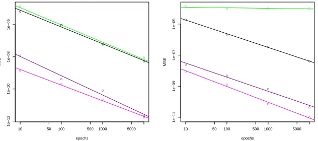
In this experiment, we compare the mean square error (MSE) for several algorithms, namely basic Zig-Zag (ZZ), Zig-Zag with Control Variates (ZZ-CV), Zig-Zag with Control Variates with a “sub-optimal” reference point (ZZ-soCV), and Stochastic Gradient Langevin Dynamics (SGLD). SGLD is implemented with fixed step size, as is usually done in practice, see e.g.
Vollmer, Zygalakis and Teh (2015), with the added benefit that it makes the comparison with the Zig-Zag algorithms more straightforward. Here in basic Zig-Zag we pretend that every iteration requires the evaluation of n
observations (whereas in practice, we can pre-compute ξMAP).
ZZ when the number of observations is increased, agreeing with the scaling results of Section5. A poor choice of reference point (as in ZZ-soCV) is seen to have only a small effect on the efficiency.
6.4. Logistic regression. In this numerical experiment we compare how the ESS per epoch (ESSpE) and ESS per second grow with the number of observationsnfor several Zig-Zag algorithms and the MALA algorithm when applied to a logistic regression problem. Conditional on a d-dimensional parameterξand givend-dimensional covariatesxj ∈Rd, wherej= 1, . . . , n,
and withxj1 = 1 for allj, the binary variableyj ∈ {0,1} has distribution
P(yj |xj1, . . . , x
j
d, ξ1, . . . , ξd) =
1
1 + exp
−Pd
i=1ξixi
.
Combined with a flat prior distribution, this induces a posterior distribution
ξ given observations of (xj, yj) forj = 1, . . . , n; see the supplementary
ma-terial for implementational details (Bierkens, Fearnhead and Roberts,2017, Section 5).
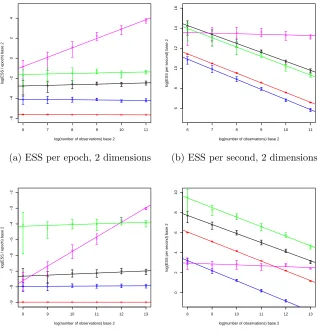
The results of this experiment are shown in Figure 3. In both the plots of ESS per epoch (see (a) and (c)), the best linear fit for ZZ-CV has slope approximately 0.95, which is in close agreement with the scaling analysis of Section 5. The other algorithms have roughly a horizontal slope, corre-sponding to a linear scaling with the size of the data. We conclude that, among the algorithms tested, ZZ-CV is the only algorithm for which the ESS per CPU second is approximately constant as a function of the size of the data (see Figure3, (b) and (d)). Furthermore ZZ-CV obtains an ESSpE which is roughly linearly increasing with the number of observationsn(see Figure3,(a) and (c)). whereas the other versions of the Zig-Zag algorithms, and MALA, have an ESSpE which is approximately constant with respect to
n. These statements apply regardless of the dimensionality of the problem.
6.5. A non-identifiable logistic regression example with unbounded Hes-sian. In a further experiment we consider one-dimensional data (xj, yj), forj = 1, . . . , n,xj ∈R,yj ∈ {0,1}, which we assume for illustrational pur-poses to be generated from a logistic model where P(yj = +1|xj, ξ1, ξ2) =
1
1+exp(−(ξ1+ξ22)xj)
. The model is non-identifiable since two parameters ξ, η
correspond to the same model as long as ξ1 +ξ22 = η1+η22. This leads to
●
●
●
●
10 50 100 500 1000 5000
1e−07 1e−06 1e−05 1e−04 1e−03 epochs MSE ● ● ● ● ● ● ● ● ● ● ● ●
(a) First moment, 100 observations
● ● ● ●
10 50 100 500 1000 5000
1e−07 1e−05 1e−03 1e−01 epochs MSE ● ● ● ● ● ● ● ● ● ● ● ●
(b) Second moment, 100 observations
●
●
●
●
10 50 100 500 1000 5000
1e−12 1e−10 1e−08 1e−06 epochs MSE ● ● ● ● ● ● ● ● ● ● ● ●
(c) First moment, 104observations ●
● ● ●
10 50 100 500 1000 5000
1e−11 1e−09 1e−07 1e−05 epochs MSE ● ● ● ● ● ● ● ● ● ● ● ●
[image:28.612.146.462.315.455.2](d) Second moment, 104observations
Figure 2: Mean square error (MSE) in the first and second moment as a function of the number of epochs, based on n= 100 or n = 10,000 obser-vations, for a one-dimensional Gaussian posterior distribution (Section6.3). Displayed are SGLD (green), ZZ-CV (magenta), ZZ-soCV (dark magenta), ZZ (black). The displayed dots represent averages over experiments based on randomly generated data from the true posterior distribution. Parameter values (see (Bierkens, Fearnhead and Roberts, 2017, Section 4)) are ξ0 = 1 (the true value of the mean parameter),ρ= 1,σ = 1 andc1= 1,c2= 1/100
● ● ● ● ● ●
6 7 8 9 10 11
−6 −4 −2 0 2 4 ● ● ● ● ● ● ● ● ● ● ● ● ● ● ● ● ● ● ● ● ● ● ● ●
log(number of observations) base 2
log(ESS / epoch) base 2
(a) ESS per epoch, 2 dimensions
● ● ● ● ● ●
6 7 8 9 10 11
6 8 10 12 14 16 ● ● ● ● ● ● ● ● ● ● ● ● ● ● ● ● ● ● ● ● ● ● ● ●
log(number of observations) base 2
log(ESS per second) base 2
(b) ESS per second, 2 dimensions
●
● ●
● ●
● ●
8 9 10 11 12 13
−9 −8 −7 −6 −5 −4 −3 −2 ● ● ● ● ● ● ● ● ● ● ● ● ● ● ● ● ● ● ● ● ● ● ● ● ● ● ● ●
log(number of observations) base 2
log(ESS / epoch) base 2
(c) ESS per epoch, 16 dimensions
● ● ● ● ● ● ●
8 9 10 11 12 13
0 2 4 6 8 10 ● ● ● ● ● ● ● ● ● ● ● ● ● ● ● ● ● ● ● ● ● ● ● ● ● ● ● ●
log(number of observations) base 2
log(ESS per second) base 2
[image:29.612.143.461.129.465.2](d) ESS per second, 16 dimensions
Figure 3: Log-log plots of the experimentally observed dependence of ESS per epoch (ESSpE) and ESS per second (ESSpS) with respect to the first co-ordinate Ξ1, as a function of the number of observationsnin the case of (2-D and 16-D) Bayesian logistic regression (Section6.4). Data is randomly gen-erated based on true parameter values ξ0 = (1,2) (2-D) and ξ0 = (1, . . . ,1)
algorithms. It is discussed in the supplementary material (Bierkens, Fearn-head and Roberts,2017, Section 6), how to obtain computational bounds for the Zig-Zag and ZZ-CV algorithms, which may serve as an illustration on how to obtain such bounds in settings beyond those described in Sections3.3
and 4.3.
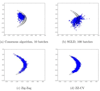
In Figure 4 we compare trace plots for the Zig-Zag algorithms (ZZ, ZZ-CV) to trace plots for Stochastic Gradient Langevin Dynamics (SGLD) and the Consensus AlgorithmScott et al.(2016). SGLD and Consensus are seen to be strongly biased, whereas ZZ and ZZ-CV target the correct distribu-tion. However this comes at a cost: ZZ-CV loses much of its efficiency in this situation (due to the combination of lack of posterior contraction and unbounded Hessian); in particular it is not super-efficient. The use of mul-tiple reference points may alleviate this problem, see also the discussion in Section7.
7. Discussion. We have introduced the multi-dimensional Zig-Zag pro-cess and shown that it can be used as an alternative to standard MCMC algorithms. The advantages of the Zig-Zag process are that it is a non-reversible process, and thus has the potential to mix better than standard reversible MCMC algorithms, and that we can use sub-sampling ideas when simulating the process and still be guaranteed to sample from the true tar-get distribution of interest. We have shown that it is possible to implement sub-sampling with control-variates in a way that we can have super-efficient sampling from a posterior: the cost per effective sample size is sub-linear in the number of data points. We believe the latter aspect will be particu-larly useful for applications where the computational cost of calculating the likelihood for a single data point is high.
As such, the Zig-Zag process holds substantial promise. However, being a completely new method, there are still substantial challenges in imple-mentation which will need to be overcome for Zig-Zag to reach the levels of popularity of standard discrete-time MCMC. The key challenges to imple-menting the Zig-Zag efficiently are
1. to simulate from the relevant time-inhomogeneous Poisson process; and
2. in order to realise the advantages of Zig-Zag for large datasets, reason-able centering points need to be found before commencing the MCMC algorithm itself.
(a) Consensus algorithm, 10 batches (b) SGLD, 100 batches
[image:31.612.139.467.117.416.2](c) Zig-Zag (d) ZZ-CV
Figure 4: Trace plots of several algorithms (blue) and density contour plots for the non-identifiable logistic regression example of Section6.5. In this ex-ample we have for the number of observationsn= 1,000. Data is randomly generated from the model with true parameter satisfyingξ1+ξ22 =−1. The
prior is a 2-dimensional standard normal distribution. Due to the unbounded Hessian and because SGLD is not corrected by a Metropolis-Hastings ac-cept/reject, the stepsize of SGLD needs to be set to a very small value (compared e.g. to what would be required for MALA) in order to prevent explosion of the trajectory; still the algorithm exhibits a significant asymp-totic bias.
we can simulate the Zig-Zag process, and also to make implementation of simulation algorithms more efficient.
The second challenge applies when using the ZZ-CV algorithm to obtain super-efficiency for big data as discussed in Subsection4.3. Although in our experience finding appropriate centering points is rarely a serious problem, it is difficult to give a prescriptive recipe for this step.
On the face of it, these challenges may limit the practical applicability of Zig-Zag, at least in the short term. With that in mind, we have released an R/Rcpp package for logistic regression, as well as the code which reproduces the experiments of Section6 (Bierkens,2017).
In addition, while Zig-Zag is an exact approximate simulation method, there are various short-cuts to speed it up at the expense of the introduction of an approximation. For instance, there are already ideas of approximately simulating the continuous-time dynamics, through approximate bounds on the Poisson rate (Pakman et al., 2016). These ideas can lead to efficient simulation of the Zig-Zag process for a wide class of models, albeit with the loss of exactness. Understanding the errors introduced by such an approach is an open area.
The most exciting aspect of the Zig-Zag process is the super-efficiency we observe when using sub-sampling with control variates. Already this idea has been adapted and shown to apply to other recent continuous-time MCMC algorithms (Fearnhead et al., 2018; Pakman et al., 2016). We have shown in Subsection6.5that Zig-Zag can be applied effectively within highly non-Gaussian examples where rival approximate methods such as SGLD and the Consensus Algorithm are seriously biased. So there is no intrinsic reason to expect Zig-Zag to rely on the target distribution being close to Gaussian, although posterior contraction and the ability to find tight Poisson process rate bounds play important roles as we saw in our examples. There is much to learn about how the efficiency of Zig-Zag depends on the statistical prop-erties of the posterior distribution. However, unlike its approximate com-petitors, Zig-Zag will still remain an exact approximate method whatever the structure of the target distribution.
algorithms isO(kn). This is confirmed by the experiment in Section6.4. The idea for control variates we present in this paper is just one, possibly the simplest, implementation of this idea. There are natural extensions to deal with e.g. multi-modal posteriors or situations where we do not have posterior concentration for all parameters. The simplest of these involve using multiple reference points and monitoring the computational bound we get within the CV-ZZ algorithm and switching to a different algorithm when we stray so far from a reference point that this bound becomes too large. More sophisticated approaches include using the ideas from (Dubey et al.,
2016), where we introduce a reference point for each data point and update the reference points for data within the subsample at each iteration of the algorithm. This would lead to the estimate of the gradient that we center our control variate estimator around to depend on the recent history of the Zig-Zag process, and thus could be accurate even if we explore multiple modes or the tails of the target distribution.
Acknowledgements. The authors are grateful for helpful comments from referees, the editor and the associate editor which have improved the paper. Furthermore the authors acknowledge Matthew Moores (University of War-wick) for helpful advice on implementing the Zig-Zag algorithms as an R package using Rcpp. All authors acknowledge the support of EPSRC under theilike grant: EP/K014463/1.
SUPPLEMENTARY MATERIAL
Supplement: Supplement to “The Zig-Zag Process and Super-Efficient Sampling for Bayesian Analysis of Big Data”
(doi: COMPLETED BY THE TYPESETTER; .pdf). Mathematics of the
Zig-Zag process, scaling of SGLD, details on the experiments including how to obtain computational bounds.
References.
Anderson, D. F.(2007). A modified next reaction method for simulating chemical sys-tems with time dependent propensities and delays.The Journal of Chemical Physics
127214107.
Andrieu, C. and Roberts, G. O. (2009). The pseudo-marginal approach for efficient
Monte Carlo computations.The Annals of Statistics37697–725.
Bardenet, R.,Doucet, A. and Holmes, C.(2015). On Markov Chain Monte Carlo
Methods for Tall Data.arXiv preprint arXiv:1505.02827.
Bierkens, J. (2015). Non-reversible Metropolis-Hastings. Statistics and Computing 25
1-16.