Munich Personal RePEc Archive
Biases and Implicit Knowledge
Cunningham, Thomas
Institute for International Economic Studies
29 September 2013
Biases and Implicit Knowledge
∗
Tom Cunningham
†First Version: September 2012
Current Version: September 2013
Abstract
A common explanation for biases in judgment and choice has been to postulate two
separate processes in the brain: a “System 1” that generates judgments automatically,
but using only a subset of the information available, and a “System 2” that uses the entire
information set, but is only occasionally activated. This theory faces two important
problems: that inconsistent judgments often persist even with high incentives, and that
inconsistencies often disappear in within-subject studies. In this paper I argue that
these behaviors are due to the existence of “implicit knowledge”, in the sense that our
automatic judgments (System 1) incorporate information which is not directly available
to our reflective system (System 2). System 2 therefore faces a signal extraction problem,
and information will not always be efficiently aggregated. The model predicts that
biases will exist whenever there is an interaction between the information private to
System 1 and that private to System 2. Additionally it can explain other puzzling
features of judgment: that judgments become consistent when they are made jointly,
that biases diminish with experience, and that people are bad at predicting their own
∗
Among many others I thank for their comments Roland Benabou, Erik Eyster, Scott Hirst, David Laibson, Vanessa Manhire, Arash Nekoei, José Luis Montiel Olea, Alex Peysakhovich, Ariel Rubinstein, Benjamin Schoefer, Andrei Shleifer, Rani Spiegler, Dmitry Taubinsky, Matan Tsur, Michael Woodford, and seminar participants at Harvard, Tel Aviv, Princeton, HHS, the IIES, and Oxford.
future judgments. Because System 1 and System 2 have perfectly aligned preferences,
welfare is well-defined in this model, and it allows for a precise treatment of eliciting
1
Introduction
A common explanation of anomalies in judgment is that people sometimes make judgments
automatically, using only superficial features of the case, ignoring more abstract or high-level
information. Variations on this type of explanation are widespread in the studies of biases
in perception, judgment, and decision-making:
• In perception the most common explanation of optical illusions is that, although the
visual system generally makes correct inferences from the information available, those
inferences are based only on local information. Pylyshyn (1999) says “a major portion
of vision . . . does its job without the intervention of [high-level] knowledge, beliefs or
expectations, even when using that knowledge would prevent it from making errors.”1
• In psychology two of the dominant paradigms, “heuristics and biases” and “dual
sys-tems”, both explain biases as due to people making judgments which are correct on
av-erage, but which use only a subset of the information (Tversky and Kahneman (1974),
Sloman (1996)).
• Within economics an important explanation of biases has been “rational inattention”
(Sims (2005), Chetty et al. (2007), Woodford (2012)). In these models people make
optimal decisions relative to some set of information, but they use only a subset of all
the information available, because they must pay a cognitive cost which is increasing
in the amount of information used.
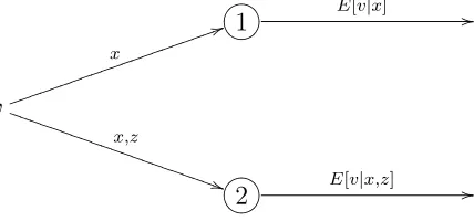
A simple version of this type of model is illustrated in Figure 1: when making judgments
we can either use an automatic system (System 1), which only uses part of the information
available, or a reflective system (System 2), which uses all the information, but is costly to
1
Feldman (2013) says “there is a great deal of evidence ... that perception is singularly uninfluenced by certain kinds of knowledge, which at the very least suggests that the Bayesian model must be limited in scope to an encapsulated perception module walled off from information that an all-embracing Bayesian account
activate.2
The names “System 1” and “System 2” are taken from Stanovich and West (2000).
In this model biases will occur when System 2 is not activated, and the nature of biases can
be understood as due to ignoring the high-level information available only to System 2.3
!"#$
%&'(1 E[v|x] !!
v x " " ❥ ❥ ❥ ❥ ❥ ❥ ❥ ❥ ❥ ❥ ❥ ❥ ❥ ❥ ❥ ❥ ❥ ❥ ❥ ❥ ❥ x,z # # ❚ ❚ ❚ ❚ ❚ ❚ ❚ ❚ ❚ ❚ ❚ ❚ ❚ ❚ ❚ ❚ ❚ ❚ ❚ ❚ ❚ !"#$
[image:5.612.199.413.152.252.2]%&'(2 E[v|x,z] !!
Figure 1: A simple representation of a two-systems model: System 1 is above, System 2 is below. Both systems form rational expectations about the unobserved variable v, however System 1 receives only x (low-level information), while System 2 additionally receives z (high-level information).
Although this class of models has been used to give persuasive analyses of individual
bi-ases, they suffer from two important empirical problems: the response of biases to incentives,
and the response of biases to joint evaluation.
First, the model predicts that biases will disappear when System 2 is activated, which
should occur whenever time and incentives are sufficiently high. Although incentives do tend
to reduce the magnitude of biases, it is commonly observed that many biases remain even
when the stakes become quite high. Camerer and Hogarth (1999) say “no replicated study
has made rationality violations disappear purely by raising incentives.” Similarly, behavior
outside the laboratory often seems to be influenced by irrelevant information even with very
high stakes (Post et al. (2008), Thaler and Benartzi (2004)). A similar point is true for
perceptual illusions: spending a longer time staring at the illusion may reduce the magnitude
of the bias, but it rarely eliminates it (Predebon et al. (1998)). Thus it becomes a puzzle
2
Although the theories listed all share the same basic diagnosis of why biases occur, they differ on a
number of other important dimensions, discussed later in the paper. More recently the System 1 / System 2 terminology has been used to refer to differences in preference (e.g. short-run vs long-run preferences), rather
than differences in information, but in this paper I just consider differences in information. 3
Within economics the terms “dual systems” and “dual selves” often refer to models in which the systems have different preferences (Fudenberg and Levine (2006), Brocas and Carrillo (2008)). In this paper I consider
why people should still be relying on their imperfect automatic judgments when there are
high incentives to not make mistakes.
Second, many experiments find that inconsistencies among judgments disappear when
those judgments are made jointly, and the two-system model gives no reason to expect this
effect. Many biases were originally identified using between-subject studies, and when tested
in within-subject studies their magnitude is generally much smaller (Kahneman and Frederick
(2005)). When valuing gambles, people often place a higher value on a dominated gamble,
but they almost never directly choose a dominated gamble (Hey (2001)). And willingness
to pay for a product can be affected by changing an irrelevant detail, but when the two
products are valued side-by-side people usually state the same willingness to pay for each
product (Mazar et al. (2010)). Overall people seem to be consistent within situations, but
their standards of evaluation change between situations.
These two generalizations - that inconsistencies are insensitive to incentives, but sensitive
to joint presentation - suggest that our reflective judgments obey principles of consistency,
but are distorted by the same biases that distort our automatic system. This could occur if
System 2’s judgment takes into account the judgments that System 1 makes. And this, in
turn, would be rational if System 1’s judgments incorporated information not accessible to
System 2.
This paper proposes that the reason we make inconsistent judgments when using our full
reflective judgment is that in different situations we receive different signals from System 1 (or
intuitions), and it is rational to take into account those signals because they contain valuable
information. I call the underlying assumption implicit knowledge, because it is knowledge
that is private to our automatic system, and thus available to our reflective system only
indirectly, through observing the automatic system’s judgments.
Figure 2 shows how the formal analysis differs: System 1 now has access to private
α
$
$
!"#$
%&'(1 E[v|x,α]
!
!
E[v|x,α]
$ $ v x " " ❥ ❥ ❥ ❥ ❥ ❥ ❥ ❥ ❥ ❥ ❥ ❥ ❥ ❥ ❥ ❥ ❥ ❥ ❥ ❥ ❥ x,z # # ❚ ❚ ❚ ❚ ❚ ❚ ❚ ❚ ❚ ❚ ❚ ❚ ❚ ❚ ❚ ❚ ❚ ❚ ❚ ❚ ❚ !"#$
%&'(2 E[v|x,z,E[v|x,α]]
!
[image:7.612.195.414.83.209.2]!
Figure 2: A two-system model with implicit knowledge: System 1 now additionally receives private information, α, and System 2 conditions its judgments on System 1’s expectation.
not be able to perfectly extract this information, and System 2’s judgment will not be the
same as if it had access to α. We can therefore define the “bias” of the two systems relative
to the benchmark case in which all the information is pooled:4
System 1’s bias = E[v|x,α]−E[v|x, z,α] (1)
System 2’s bias = E[v|x, z, E[v|x,α]]−E[v|x, z,α] (2)
Equation (2) forms the centerpiece of this paper, it represents the bias due to the fact
that some of our knowledge is implicit.
System 1’s private information,α, can be interpreted as either static or dynamic
informa-tion. In most of this paper I assume that it is static, i.e. it represents long-run information
about the state of the world, and how to interpret x, known only to System 1.5
As far as I know this is the first formal model of the influence of implicit knowledge in
decision-making.6
Appealing to implicit knowledge may seem exotic, but there are good
4
This Bayesian definition of “bias” is meant to capture the usual use of the word in the judgment and decision-making literature. It is different from “bias” in the econometric sense, where an estimatorvˆ(α, z)
would be unbiased ifE[ˆv(α, z)|v] =v. An estimate which is unbiased in the Bayesian sense can be biased in
the econometric sense, and vice versa.
5
If α were dynamic it would represent information about the current situation available only to the
automatic system, i.e. subconsciously perceived cues. There may be cases where this plays a role in judgment, but I leave this aside in the present paper.
6
reasons to believe that large parts of our knowledge are only accessible in limited ways. In
perception the evidence is overwhelming: our eyes are able to make very accurate inferences
from the light they receive, but it has taken psychologists a centuries to understand how those
inferences are made, and the best computers remain inferior to a small child in interpreting
photographs. In more general knowledge a striking pattern is that we are far better at
recognizing certain patterns thanreproducing them. As a simple example, most people find
it difficult to answer the question “is there an English word which contains five consecutive
vowels?”, but instantly recognize that the statement is true when they are reminded of a word
that fits the pattern.7
Most people can easily recognize whether a sentence is grammatical,
but have difficulty making generalizations about the set of grammatical sentences.8
These
distinctions in accessibility would not exist if our knowledge was explicit, i.e. stored as a
distribution over possible states of the world. This paper proposes that the knowledge we
use in making economic decisions is stored in a similarly implicit form: that people are able
to make confident snap judgments about the value of different alternatives, but they have
limited insight into how those judgments are formed. This separation of knowledge between
systems can explain why our decisions often violate normative principles that we reflectively
endorse.
The model makes a variety of predictions about human judgment: (1) biases will occur
when there is an interaction between implicit knowledge and high-level information in
infer-ring v (i.e., between α and z); (2) judgments will appear inconsistent to an outside observer
because in different situations the reflective system will have different information about α;
(3) biases will be systematic, such that it will appear as if people are using simple
heuris-tics; (4) however when making multiple judgments jointly then judgments will be consistent,
because they will condition on the same beliefs about α; (5) the magnitude of biases will
7
“queueing”.
8
decrease when a person is given more cases to judge, because with a larger set they can
learn more of the information that is private to their automatic system; and (6) people will
not be able to accurately predict their future judgments, because they cannot anticipate the
estimates that System 1 will produce in future situations.
I discuss evidence relevant to these predictions from perception, judgment, and economic
decision-making. In particular I emphasize the interpretation of framing effects: the reason
that we can be influenced by irrelevant features of the situation (anchors, reference points,
decoy alternatives, salience) is because those features are ordinarily relevant, and therefore
influence our automatic judgments. Even when we know a feature to be irrelevant in the
current case, it nevertheless can affect our reflective judgment indirectly because its influence
on automatic judgment is combined with other influences that are relevant, therefore we
often cannot completely decontaminate our automatic judgments to get rid of the irrelevant
influence.
Framing effects are often interpreted as evidence that true preferences do not exist, or
that preferences are labile, posing an important challenge to welfare economics (Ariely et al.
(2003), Bernheim and Rangel (2009)). The interpretation of this paper is that framing effects
reflect problems with aggregation of knowledge, and therefore true preferences do exist, and
can be recovered from choices. The model makes predictions about how true preferences can
be recovered: in particular, it predicts that judgments can be debiased by presenting subjects
with comparisons that vary the aspects that are irrelevant, allowing subjects to isolate the
cause of their bias.
The model in this paper differs qualitatively from existing models of imperfect attention
or imperfect memory, in fact it is the interaction of these two mechanisms that generates
biases (System 1 has imperfect attention, System 2 has imperfect memory). The model is
most related to the literature on social learning and herding, in which each agent learns from
observing prior agents’ actions. This paper makes three significant formal contributions.
the distribution of information between agents. Second, under the assumption that the first
agent’s private information is static, it shows under what conditions judgments and decisions
will be consistent when made jointly. Third, it presents an analytic solution for the bias under
linear-Gaussian assumptions, allowing for a clear intuitive characterization of how implicit
and explicit knowledge interact to affect judgment.
The interpretive contribution of this paper is to argue that many biases - in
percep-tion, judgment, and choice - are best understood as being due to the existence of implicit
knowledge.
1.1
Metaphor
A simple metaphor can be used to illustrate all of the principal effects in the model: the
model predicts that behavior will be as if you had access to an oracle who had superior
memory (i.e., which knows α), but which also has inferior perception of the situation (i.e.,
they do not observe z).
To be more concrete, suppose that you were attending an auction of baseball cards, and
suppose that you were accompanied by your sister, who will represent System 1. Suppose
that your sister has superior memory, meaning that she has a superior knowledge of the value
of individual baseball cards. However suppose that she has inferior perception, which will
mean that she cannot discriminate between genuine and fake cards.
When confronted with a packet of cards your sister will announce the expected value
of those cards, according to her experience, but without knowing whether any of the cards
are fake. Because you know which cards are fake you will wish to adjust her estimate to
incorporate your own information, however because her estimate is of the value of an entire
packet you cannot exactly back out her estimates of the values of individual cards. Your
final judgment will therefore be influenced by your sister’s knowledge, but it will not be an
optimal aggregation of your own information with your sister’s.
partic-ular, your bids will be affected by information that you know to be irrelevant. Consider two
packets which are identical except for the final card: one contains a forged Babe Ruth card,
and the other contains a forgedTy Cobb. In each case the sister would give the packets diff
er-ent estimates because she is not aware that they differ only in cards which are fake. Because
you are not able to infer your sister’s knowledge of the values of the individual cards, the
value of the fake card will indirectly influence your judgment in each case, and you would
produce different bids in each of the two situations.
The outside observer would conclude that your judgment is biased: your behavior is as
if you are following a heuristic, i.e. ignoring whether or not cards are genuine. However
the observer would also notice a striking fact: that your judgments will obey principles
of consistency when multiple packets are considered simultaneously. Suppose that the two
packets described above are encountered at the same time. The sister will give two different
estimates. However upon hearing these two estimates you will update your beliefs about the
values of all of the cards, and your two bids will be identical, because they reflect the same
beliefs about card values.
Two more of the predictions can be illustrated with this metaphor. First, exposure to a
larger set of cases will tend to reduce biases: if you are presented with a set of packets, and
you can hear your sister’s estimates for each packet, then you will be able to infer more of
your sister’s knowledge, and your bias will decline, converging towards a situation in which
you learn all of your sister’s knowledge. Second, the model predicts that people will not be
able to accurately forecast their future judgments. For example, suppose you were asked to
choose a set of 3 cards worth exactly $100, and you made this choice without your sister’s help
(i.e., your sister refuses to share her knowledge, apart from stating her estimates of individual
packets). You may choose a set of cards which you believe is worth $100 under your current
knowledge, but when you present that packet to your sister, and hear her estimate, your
estimate is likely to change.
exist, when we can predict the direction of the bias, how it is affected by comparing multiple
cases, and I show that inconsistencies will disappear in joint evaluation. In the following
section I present a version of the model with functional-form assumptions, allowing for a
precise discussion of how implicit knowledge, low-level and high-level information interact
in producing judgment biases. Following the exposition of the models I discuss existing
literature in psychology and economics which argues for the two systems interpretation of
biases shown in Figure 1, and evidence relevant to the novel predictions of the model. In the
conclusion I discuss related literature, extensions, application to well-known anomalies, and
welfare implications. An appendix contains all the proofs not in the body of the paper.
2
Model
Assume a probability space (Ω, E, P), and four random variables v ∈R, x ∈X, z ∈Z, α ∈
A, defined by the measurable functions Fv : Ω → R, Fx : Ω → X, Fz : Ω → Z, and
Fα : Ω → A. I define a joint distribution measure f(v, x, z,α)≡ P({ω|Fv(ω) = v, Fx(ω) =
x, Fz(ω) = z, Fα(ω) = α}), and conditional distributions derived from that.
We can then define the following expectations, which represent respectively the
expecta-tions about v formed by System 1, by System 2, and by a hypothetical agent who is able to
pool both information sets:
E1 = E[v|x,α]
E2 = E[v|x, z, E[v|x,α]]
EP = E[v|x, z,α]
expecta-tion that would have been produced had both stages pooled their informaexpecta-tion:
System 1’s bias = E1−EP
System 2’s bias = E2−EP
Both E1 and E2 will have a zero average bias, i.e. E[E1 −EP] =E[E2 −EP] = 0, however
System 2 will have a smaller bias on average:
Proposition 1. System 2 has a smaller average bias (by mean squared error)
E!
(E2−EP)2
"
≤E!
(E1−EP)2
"
This follows, indirectly, from the fact that the variance of an expectation’s error will be
smaller if it conditions on more information:
Lemma 1. For any random variables v, p, q:
V ar[v−E[v|p, q]]≤V ar[v−E[v|p]] (3)
System 2’s expected bias may not be smaller by a different measure (e.g., by absolute
value), however the squared bias is the natural measure of magnitude in this model since the
expectation minimizes the squared error. Another quantity of interest is the estimate which
would be produced by System 2 without access to System 1’s output, I will denote this by:
E2\1 =E[v|x, z]
I discuss the interpretation of this quantity later in the paper, but note that the average bias
of E2\1 will be higher than the bias of E2 by Lemma 1.
Finally, I will assume that a separate mechanism decides whether or not to activate
π ∈R. Then we can define a final expectation which is used for decision-making:
EF =
E1 π<π¯
E2 π≥π¯
where π¯ ∈ R is a constant. This describes the behavior of a person who activates System 2
only when the incentive is sufficiently high. This will be a rational strategy for an agent who
faces a loss function which is quadratic in (EF −v), and who must pay a cost when System
2 is activated.9
In practice mental effort may lie on a continuum, rather than being binary. What is
important for this model is that even with maximum mental effort, not all information is
efficiently aggregated.
In the rest of the paper I concentrate mainly on the properties of System 2’s bias,E2−EP,
i.e. the bias which survives in a person’s reflective judgment. When I say that judgment is
unbiased I will mean that for all x∈X,α∈A, z ∈Z,
E[v|x, z, E[v|x,α]] = E[v|x, z,α]
2.1
Conditions for a Bias in Reflective Judgment
A simple sufficient condition for unbiasedness is thatE[v|x,α]is a one-to-one function of α.
If it was then System 2 would simply be able to invert E1 to inferα. However this condition
is not necessary, because in many cases System 2 can extract all the information it needs
from E1 without knowingα. We are able to give more interesting conditions below.
The relationship between E1, E2, and EP can be illustrated in the following table:
9
A more sophisticated model would allow this decision to condition on more information (x, z, and perhapsα), but for the purposes of this paper it is only important that there is some level of incentives above
α α′ α′′
z E[v|x, z,α] E[v|x, z,α′] E[v|x, z,α′′] z′ E[v|x, z′,α] E[v|x, z′,α′] E[v|x, z′,α′′]
E[v|x,α] E[v|x,α′] E[v|x,α′′]
In this table each column represents a different realization of α, and the rows represent
realizations of z. The six interior cells correspond to the pooled expectation, EP, under
different realizations of α and z. The elements of the last row correspond to E1, i.e. they
are average expectations conditioning only on α. Finally, the two cells surrounded by a
border correspond to a realization of E2, i.e. a set of cells in a row grouped according to
whether their columns share the same E1: here the border is drawn under the assumption
that E[v|x,α] =E[v|x,α′](=E[v|x,α′′].
A bias occurs when E2 (= EP, thus in the table it will occur when the rectangle
rep-resenting E2 encompasses cells with different values. A necessary and sufficient condition
for unbiasedness will be that any columns which share the same average (E1) must also be
identical for every cell.
Proposition 2. Judgment will be unbiased if and only if, for allx∈X, α,α′ ∈A,
E[v|x,α] =E[v|x,α′] =⇒ ∀z ∈Z, E[v|x, z,α] =E[v|x, z,α′]
To illustrate I give an example where aggregation of information fails (xis ignored in this
example).
Example 1. Letv,α, z ∈{0,1}, withf(v = 1) = 1
2. Suppose that ifv = 0 thenα and z are
uniformly distributed and independent, but if v = 1then with equal probability α =z = 1, or α=z = 0. I.e., for all α, z ∈{0,1}:
f(α, z|v = 0) = 14 f(α, z|v = 1) =
1
Then we can write:
EP =E[v|α, z] =
2
3 , α=z 0 , α(=z
= 2
3(1−α−z+ 2αz)
E1 =E[v|α] = 1
'
z=0
E[v|α, z]f(z|α)
= 0×1
4 + 2 3 ×
3 4 =
1 2 E2 =E[v|E[v|α], z] =
1 2
Here the pooled-information expectation includes an interaction term between α and z. In
this case we do not know whether a realization of α represents good news or bad news about
v until we know the realization of z. In fact, in this case it means that the intermediate
expectation, E1, will be entirely uninformative, because E1 = 12 everywhere, independent of
α. System 2 cannot learn anything about α, so both System 1 and 2 will be biased relative
to the pooled-information benchmark (i.e., ∀α∈A, z ∈Z, E1 =E2 (=EP).
We are able to give a more intuitive condition for unbiasedness under the assumption that
α and z are independent. This assumption seems reasonable in the preferred interpretation
of the model where α represents long-run knowledge (i.e., knowledge about how to interpret
x), and z represents idiosyncratic high-level information about the current case.
When α and z are independent, then judgment will be (almost surely) unbiased if α is
monotonic, in the sense that a change fromα toα′ is either always good news (i.e., it weakly
increases the expected v for every z), or always bad news.
Proposition 3. Judgment will be almost surely unbiased ifα andz are independent, and if,
for every x∈X, there exists some total order ,x on A, such that for all z ∈Z, E[v|x, z,α] is weakly monotonic in α when ordered by ,x.
way that the elements in every row are weakly increasing.
A natural case in which bias will occur is ifαrepresents a vector of continuous parameters,
andz represents information on how much weight to put on each element in the vector (these
are the assumptions used in the Gaussian model discussed below). Because α is a vector,
E[v|x,α] may not be invertible. And because the relative importance of different elements
of α depends on the realization of z, then α will not be monotonic, i.e. α′ may be better or
worse than α (in terms of v) depending on the realization ofz.
It follows from proposition 3 that bias will not occur when EP is a separable function of
α and z, i.e. there must be some interaction between the two pieces of information for bias
to occur.
Corollary 1. Judgment will be unbiased ifαandz are independent, and there exist functions
g :X×A→R, h:X×Z →R, and i:R→R, such that
EP =E[v|x, z,α] =i(g(x,α) +h(x, z))
and i is strictly monotonic.
Proof. In this case for any x there exists an ordering of A such that EP is monotonic in α,
for any z (i.e., the ordering according to g(x,α)). Judgment will therefore be unbiased, by the previous proposition.
The existence of bias is sensitive to the distribution of knowledge: for example, no bias
would occur if your sister knew everything about the half of the baseball cards that are
alphabetically first, A-M, and you knew everything about the second half of baseball cards,
N-Z. If your sister knows both the values of her cards, and how to spot a fake, then changes
in your sister’s knowledge would then be monotonic: a change would be unambiguously good
or unambiguously bad news, independent of System 2’s knowledge, and therefore there would
In a related paper Arieli and Mueller-Frank (2013) show that there will be no bias if the
signalsαand z are conditionally independent (givenv andx), and if System 2 can infer from
E1 the entire posterior of System 1, not just their expectation (i.e. if they can inferf(v|x,α), not just E[v|x,α]). They also show thatE1 will almost always reveal the entire posterior, in a probabilistically generic sense. The latter fact will hold in the Gaussian examples below:
System 2 always will be able to infer System 1’s entire posterior distribution overv. However
in most examples of interest to this paper αandz will not be conditionally independent, and
for this reason Arieli and Mueller-Frank’s theorem will not apply, and a bias will remain.
2.2
Multiple Evaluations
An important distinctive prediction of this model is regarding judgments made jointly.
Most models of judgment and choice assume that each case is evaluated separately,
inde-pendent of other cases that may be under consideration at the same time.10
However I will
assume that when a set of cases is is encountered jointly then the reflective system receives
a corresponding set of automatic judgments, and that it can use the information from the
entire set to learn more about α, and therefore more about each individual case. To represent
joint evaluations I consider vectors ofm∈N+ elements, v=Rm,x=Xm,α=Am,z=Zm,
with the joint distribution,
fm(v,x,z,α)
I will refer to a pair of vectors (x,z) as a situation, and an element (xi, zi) as a case. I
assume that System 1 forms their expectations about each case as before, and that System 2
conditions each of their judgments on the entire set of expectations received from System 1,
10
Exceptions include theories of choice with menu-dependent preferences, e.g. Bordalo et al. (2012), Kőszegi and Szeidl (2011), or where inferences are made from the composition of the choice set, Kamenica
E1 = E[v|x,α]
E2 = E[v|x,z,E1]
EP = E[v|x,z,α]
As written, this setup allows many channels of inference, so I introduce further assumptions
in order to concentrate just on the channels of interest.
First, as discussed, our principal interpretation is that System 1’s private information
represents long-run knowledge, so I assume that all elements of αare identical, and therefore
simply refer to it as α.
Second, I will assume that each case (xi, zi) is distributed independently of α. If the
elements of x were informative about α then we would expect joint and separate judgment
to differ even without any signal from System 1.11
Finally, we will also assume that all observable information about each object is
idiosyn-cratic, i.e. xi and zi are informative only about vi, not about vj for j (=i.
These three points are incorporated into the following assumption about the distribution
of information:
fm(v,x,z,α) =
( m )
i=1
f(vi|xi, zi,α)
*
f(z|x)f(x)f(α) (A1)
We can first note that, within this framework, neither System 1’s expectation nor the
pooled-information expectation will differ between joint and separate evaluation, i.e.:
E1i = E[v|xi,α]
EPi = E[v|xi, zi,α]
However when System 2 observes a vector E1, it can learn aboutα from the entire set of
11
cases. Therefore, for any given case, an increase in the number of other cases evaluated at
the same time will reduce the expected bias:
Proposition 4. For any m < n, x ∈ Xm, z ∈ Zm, x′ ∈ Xn, z′ ∈ Zn, with xi = x′i and
zi =z′i
for i∈{1, . . . , m}, then for any j ∈{1, . . . , m}
V ar[E2j−EPj]≥V ar[E2′j −EP′j]
where E2 =E[v|x,z, E[v|x,α]] and E′
2 =E[v′|x′,z′, E[v|x′,α]].
Proof. Because the first expectation conditions on a strictly larger information set, the result
follows from Lemma 1.
This proposition can be interpreted as applying to sequential, as well as joint, evaluation.
Suppose that an agent evaluates(x, z)and(x′, z′)in sequence, and assume that when System
2 evaluates the second case it has access to E1 for both cases – in other words, assume that
the decision-maker can remember their intuitions for previous cases, at least for a short
time. Then System 2’s second judgment will be the same as if they evaluated the pair
(x,z) = ((x, x′),(z, z′))simultaneously, and therefore the expected bias will decrease relative
to the case in which (x′, z′)is evaluated without any history. In other words, more experience
is predicted to reduce the bias.
To apply this prediction about sequential judgments requires interpretation of when a
set of cases are part of the samesituation. The important assumption is that System 2 can
recall all previous stimuli (x, z), and previous judgments (E1), so one natural application is
to laboratory experiments in which subjects make a series of decisions in quick succession.
To give some intuition for this result consider the problem of choosing a house to buy.
You might view one house, and get a good feeling about it, but not be sure what aspects
of the house contributed to that feeling. As you visit more houses you come to learn more
about what makes you like a house. And you may discover that your feelings are affected by
house if the sun was shining on the day you visited it. As you discover this pattern in your
judgments you learn to discount your intuitions to account for the weather, and the quality
of your judgment will increase (i.e., the accuracy of your judgments of the intrinsic quality
of a house will improve). In this case more experience will decrease bias.
2.3
Consistency
I now show how these results regarding the size of bias can be interpreted as predictions
about consistency of judgments. In studying human judgment it is often difficult to say
that a single judgment is biased, because bias is relative to a person’s beliefs, and it is
difficult to observe their full set of beliefs. We often establish bias indirectly by showing that
judgments, individually or collectively, violate some restriction which unbiased judgments
ought to satisfy. For example, it is difficult to demonstrate that a subject over-values or
under-values a particular good, but many experiments demonstrate that valuation is affected
by normatively irrelevant details. Other experiments show that judgments indirectly violate
dominance (e.g. List (2002)), or transitivity (Tversky and Simonson (1993)).
The model in this paper makes a clear prediction: people may violate the normative
principles of consistency in separate evaluation, but will satisfy them if the same cases are
evaluated jointly; put another way, they mayindirectly violate axioms of rational choice, but
will not directly violate them. For example, choices may be intransitive, but people would
never choose a dominated alternative. Also, choices made separately may be inconsistent,
but choices made jointly (assumed to condition on the same set E1) will obey any restrictions
on choice.
To state this proposition we introduce the concept of a restriction on judgment. Let a
judgment function be a function u : X ×Z → R. In some cases I will interpret this as a
utility function, in which the unknown utility of an object is inferred from its features.12
One
simple restriction on judgment is, for example, that two cases (x, z) and (x′, z′) should be
12
given the same evaluation; this can be expressed as a subset of the set of possible judgment
functions, {u:u(x, z) =u(x′, z′)}. We will be interested only in convex restrictions, i.e.:
Definition 1. A restriction on judgmentU ⊆RX×Z is convex if and only if, for anyu, v ∈U, and 0<α<1,
αu+ (1−α)v ∈U
If a restriction is convex then it means that any linear mixture of judgment functions which
each satisfy a constraint will itself satisfy the constraint. Most common restrictions satisfy
this definition, e.g. indifference between pairs of alternatives, dominance between pairs, or
separability of arguments.13
It is convenient to define judgment functions corresponding to
the the three types of expectation:
uα
1(x, z) = E[v|x,α] uα
2(x, z) = E[v|x, z, E[v|x,α]] uα
P(x, z) = E[v|x, z,α]
It will also be convenient to define a joint judgment function for System 2, which conditions
on a set of cases, x,14
uα,x
2 (x, z) =E[v|x, z, E[v|x,α]].
Now suppose that the pooled-information judgment function uα
P satisfies some convex
restriction U. Clearly uα
1 may violate that restriction, because it ignores z. However for u2
the result will be mixed: when evaluations are made separately (i.e., when conditioning on
different setsx), then the restriction may be violated, but when evaluations are made jointly,
with the same conditioning set x, they will always satisfy the restriction.
13
For example, the indifference restriction{u:u(x, z) =u(x′, z′)}is convex because any mixture between
pairs of utility functions which satisfy this indifference will itself satisfy indifference. An example of a
non-convex restriction is thatu(x, z)∈{0,1}.
14
This represents the evaluation ofxconditioning on some other setx. In practice we may only observe
Proposition 5. For any convex restriction on judgmentU ⊆RX×Z with, for allα∈A,
uα
P(x, z)∈U
then for all α ∈A, x∈Xm, m >1,
uα,x
2 (x, z) ∈U
For example consider how people will respond to irrelevant differences. Suppose that
our restriction is, as above, that for some x, x′ ∈ X, z, z′ ∈ Z, {u : u(x, z) = u(x′, z′)}.
Proposition 5 implies that people evaluating (x, z) and (x′, z′) jointly will evaluate them to
have the same worth, though they may give different judgments when evaluated separately.
A natural corollary exists in choice behavior. Usually we assume that choice from a choice
set (D∈D, D= 2X×Z\∅) is generated by maximizing a utility function:
c(D) = arg max (x,z)∈D
u(x, z)
and restrictions on the utility function can be translated into restrictions (or axioms) on
the choice correspondence. Choice correspondences can be defined corresponding to each
evaluation function defined above (i.e. cα
P,cα1, cα2, c
α,x
2 pick out the maximal elements of the
choice set according to the functions uα
P, uα1, uα2, and u
α,x
2 ). In the case of c
α,x
2 I make the
further assumption that the conditioning set xis formed by elements of the choice set,D, i.e.
that when choosing from a choice set, System 2 receives signals from System 1 about each of
the alternatives in the choice set. Proposition 5 will imply that, if EP satisfies some convex
restriction U, then System 2’s choices will obey any axioms implied by that restriction.
Corollary 2. For any convex restriction on judgment,U ⊆RX×Z, and corresponding choice restriction CU ⊆ DD,
15
if pooled-information judgment satisfies U (∀α ∈ A, uα
P ∈ U) then
15
individual System 2 choices will satisfy CU.
Proof. By the proposition, each uα,x
2 belongs to U, therefore it must satisfy the choice
re-strictions implied by U.
Decisions made by System 1 may violate restrictions axioms on choice, because those
decisions will fail to condition on z (put another way, inattentive decisions may violate
axioms of choice). Proposition 5 implies that System 2’s decisions will never violate an
axiom in a given choice set, although decisions made separately can collectively violate those
axioms. If the underlying restriction U entirely rules out certain choices, then those choices
will never be made by System 2. For example if U included a dominance restriction, so
that for some (x, z),(x′, z) ∈ X ×Z, U = {u : u(x, z) > u(x′, z)}, then a decision-maker
with implicit knowledge would never choose a dominated option ((x′, z)∈c({(x, z),(x′, z)})),
however they might still make intransitive choices (e.g. (x, z) =c({(x, z),(x′, z)}), (x′, z) =
c({(x′, z),(x′′, z)}), (x′′, z) =c({(x′′, z),(x, z)})).
This can be extended to choices which are made jointly. Joint decision-making is a
common protocol used in experiments (Hsee et al. (1999), Mazar et al. (2010)). Subjects
are typically instructed to consider all choice sets before making their several decisions,
and are told that a single decision will be randomly chosen to be implemented. If choices
obey the independence axiom of expected utility theory, and subjects infer nothing from the
composition of the choice set, then choice from each given choice set should be unaffected by
the other choices being considered simultaneously.
The corollary above implies that choices made jointly will not violate any axioms of choice,
under the assumption that when presented with joint choices people make judgments which
condition on all the alternatives available. To be precise, if they are confronted with a set of
choice sets D1, .., Dn, then I assume that they form judgments using E2α,x, withxnow being
the union of all the choice sets (i.e., x∈x iff x∈D1∪. . .∪Dn).
It is important to emphasize that although the model predicts that joint evaluations
E2 = EP). In terms of baseball cards, consistency implies giving two packets the same
bid when they differ only in a counterfeit card. Though consistent, these judgments may
still have bias: even in joint evaluation you will not necessarily be able to back out perfect
knowledge of α from your sister’s reports, so your judgments may still be biased relative to
the pooled-information benchmark.
It is also worth mentioning that choices taken sequentially need not be consistent with
each other.16
Later choices will have access to larger sets of E1 judgments, and therefore
different beliefs about α, thus sequential decisions need not be consistent.
2.4
Learnability
In its current form the model allows for the existence of knowledge held by System 1 which
could never be discovered by System 2. Suppose there exist a pair α,α′ ∈ A such that, for every x ∈ X, E[v|x,α] = E[v|x,α′]. Then System 2 could never discover whether α or α′
holds, even though it may be relevant, i.e. ∃z ∈Z, E[v|x, z,α](=E[v|x, z,α′].
In this section I note that if α is learnable by System 1 (in a particular sense) then α
can also be inferred by System 2, from observing System 1’s responses. Therefore there will
be no bias when System 2 observes all of System 1’s judgments, i.e. its judgments for every
possible x.
Definition 2. A distributionf(v, x, z,α)is learnable if ∀α,α′ ∈A, ∃x∈X,
E[v|x,α](=E[v|x,α′]
Learnability is a natural restriction if we think of System 1 as a naive learner: i.e., if
System 1 simply stores the average observed v for a given x. Given an unlearnable
distribu-tion, there will always exist a coarsening of A that is learnable (because, at worst, if A is a
16
singleton, then it is learnable).17
The following proposition states that if System 2 can observe System 1’s judgment for
every element in X, and f is learnable, then judgment will be unbiased.
Proposition 6. If f is learnable then for all α ∈ A, z ∈ Z, x ∈X, m ∈N, x∈ Xm, with
x′ ∈x ⇐⇒ x′ ∈X,
Eα,x
2 (x, z) =EPα(x, z)
Proof. Becausexcontains every element inX, thenE1will containE[v|x,α]for everyx∈X.
Because f is learnable, there is only a single α∈A that is consistent with this pattern, thus
E[α|x,E1] =α. Therefore E2 =E[v|x,z,E1] =E[v|x,z,α] =EP.
2.5
Comparative Statics
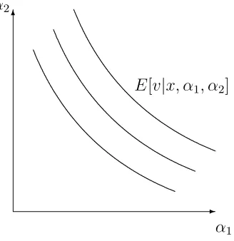
Next we consider what can be said about the direction of the bias. An illustration of the
nature of the problem is given in Figure 3, in which System 1’s private information is a
point in a two-dimensional space ((α1,α2) ∈ A = R2), and E[v|x, z,α1,α2] is assumed to be increasing in both α1 and α2. System 1 observes (α1,α2) and calculates an expectation,
E1 = E[v|x,α1,α2]. System 2 observes that expectation, and therefore learns that α1 and
α2 lie on a certain curve, which leads him to update his posterior over (α1,α2). A natural
assumption will be that, when System 2 observes a higher E1, his posteriors over both α1
and α2 increase, in the sense of having higher expected values. If this is true then there will
be a “spillover” effect: an increase in α1 will cause an increase in System 2’s estimate of α2.
Thus in situations where α1 is known to be irrelevant, it will nevertheless affect System 2’s
judgment, and the direction of influence will be predictable.
If this property holds we can tell an intuitive story about biases: even when System 2
17
There is a simple example of a non-learnable distribution for the baseball-cards example. Suppose the distribution of cards is such that two cards P and Q only ever appear together, i.e. every pack contains either both cards or neither. Then someone who observesxandv will not be able to learnα(the values of
the cards). In particular for any assignment of values to P and Q which is consistent with the observedx
✻
✲ α1
α2
[image:27.612.226.390.50.219.2]E[v|x,α1,α2]
Figure 3: Isovalues in System 1’s judgment.
knows that α1 is irrelevant (i.e., under some realization of x and z, α1 is unrelated to v),
nevertheless System 2’s judgment will be a monotonic function of α1. For example, when you
know that the Babe Ruth card is counterfeit, your bid will be nevertheless increasing in the
value of that card, because its value indirectly affects your judgment through your sister’s
report of the value of the packet.
A simple example is if EP =α1z1 +α2z2, with α1 and α2 having Gaussian distributions,
and with(α1,α2, z1, z2)all distributed independently. ThenE1 =α1E[z1] +α2E[z2], and the
inferred α1 and α2 will both be monotonic in E1.
I define this property as unambiguousness, meaning that a change in α which increases
E1 will weakly increase E2, for all values of x and z:
Definition 3. A distributionf(v, x, z,α)is unambiguous if, for anyx∈X,α,α′ ∈A,z ∈Z,
E[v|x,α′]> E[v|x,α] =⇒ E[v|x, E[v|x,α′], z]≥E[v|x, E[v|x,α], z]
Unambiguousness is related to the monotone likelihood ratio property (Milgrom (1981)):
a distribution is unambiguous when a higher E1 causes System 2 to infer a higher v, no
matter the realization of z.
increase in E1 will cause System 2 to increase their posteriors over every αi (in the sense of
stochastic dominance), which in turn implies that f is unambiguous.
Proposition 7. If A=Rn, α and z are independent, and
E1 =E[v|x,α] =
n
'
i=1
αig(x)
and each αi is distributed independently with F(αi|x) differentiable and f(αi|x) log-concave, and E[v|x,α, z] is increasing in α, then f is unambiguous.
Proof. Shaked and Shanthikumar (2007) Theorem 6.B.9 establishes that the posteriors over
αi will increase inE1, in the sense of stochastic dominance. Because EP is increasing in each
α, thenE2 must increase, thus f is unambiguous.
2.6
E
ff
ects of the Common Information
We have discussed how changes in System 1’s private information, α, affect System 2’s
judgment. We now discuss changes in the common information,x, which allows us to address
how biases may depend on aspects of the given case.
In particular, a common explanation for judgment being sensitive to a normatively
ir-relevant change is that, although the change is irir-relevant in the current situation, it is
usually relevant, i.e. it is relevant in other similar situations. This is a common
“heuris-tics” explanation of biases. In the terms of this paper, a change in low-level
informa-tion (x to x′) may be normatively irrelevant given the high-level information z, for all α,
E[v|x, z,α] = E[v|x′, z,α], but the change is informative if we ignore the high-level
informa-tion, for some α, E[v|x′,α]> E[v|x,α].
This can explain why System 1 makes a mistake, however to explain why System 2 can
be biased requires implicit knowledge. It also remains to be shown under what conditions
under what conditions will a change in xwhich causes an increase inE1 also cause a (weak)
increase in E2? I call this property congruence:
Definition 4. A distributionf is congruent for some x, x′ ∈X, andz ∈Z if,
∀α ∈A, E[v|x′,α]> E[v|x,α] =⇒ E[v|x′, E[v|x′,α], z]≥E[v|x, E[v|x,α], z]
This may not hold even if f is unambiguous in the sense defined above. There are two
qualifications. First, if System 2 knows that x′ is associated with a higher v than x, then
it will already discount the effect on E1. Therefore we are really interested in the difference
between what each System believes about the relationship between x and v. A natural
benchmark is when System 2 expects no difference: i.e., whenE[v|x′] =E[v|x]. Second, even
if System 2 has the same expectation about v given x and x′, still congruence may fail if
the variance differs between cases. For example, suppose that System 2 was relatively more
uncertain about the relationship between x′ andv, then it would discount the signal fromE
1
relatively more, and this discounting effect could overwhelm the principal effect.18
We can show that a change in x will cause congruent changes in E1 and E2 under
as-sumptions of orthogonality and symmetry. Suppose that under some realization z ∈Z, two cases x and x′ have the same value. Then we can partition the space of A into relevant and
irrelevant information (i.e., partition Ainto A1×A2, depending on whether it has any effect
on E[v|x,α, z]). If we assume that (1) the relevant and irrelevant information is distributed independently; and (2) forxandx′, the irrelevant information is distributed identically; then
18
Suppose that replacingBabe Ruth withTy Cobb increasesE1. If System 2 knows that both cards are fake, then he wishes to infer, fromE1, only the part ofαwhich is relevant to the remaining genuine cards. If
his priors over the values ofBabe Ruth andTy Cobb have the same shape, then this inference should be the same, i.e. replacingBabe RuthwithTy Cobbwill have the same effect as if the value ofBabe Ruthincreased
to be equal to that of Ty Cobb. And if f is unambiguous, the change in E1 has a congruent effect on E2. However this conclusion could be reversed if System 2 had a relatively larger uncertainty about the value of
Ty Cobb. As the variance of System 2’s prior onTy Cobb increases, then E1becomes less informative about the part ofαrelevant to System 2 (i.e., the part ofαrelevant to the genuine cards), and System 2 will put
relatively more weight on his prior, and relatively less weight onE1. In the limit, as System 2 becomes more uncertain aboutTy Cobb’s value, he will eventually ignore the signal from System 1, and therefore even when
the changes in E1 and E2 will be congruent (iff is unambiguous).
Proposition 8. For any x, x′ ∈X, and z ∈Z, if
(i) under z, the difference between x and x′ is irrelevant, i.e. ∀α ∈ A, E[v|x, z,α] =
E[v|x′, z,α]
(ii) A can be divided into two parts, distributed independently of each other and of x, i.e.
A=A1×A2, withf(α1,α2, x) =f(α1)f(α2)f(x)
(iii) under z, α2 is irrelevant, i.e. E[v|x′′, z,α1,α2] = E[v|x′′, z,α1,α′2] for all x′′ ∈ X,
α1 ∈A1, α2,α′2 ∈A2
(iv) given α1, x and x′ have the same information about v, i.e. ∀α1 ∈ A1, f(v|x,α1) = f(v|x′,α
1)
(v) f is unambiguous
then the distribution f will be congruent for x and x′.
This result allows us to derive an important prediction: if we observe bias to go in a
particular direction, then we should expect the world to also move in that direction. I.e., if
x′ induces a higher judgment than x, even when people know that the difference is
norma-tively irrelevant, then, under the assumptions above, this implies that E[v|x′,α]> E[v|x,α],
i.e. that on average (ignoring z) x′ is associated with higher v, though people may not be
consciously aware of this association. I discuss evidence for this prediction in a later section.
3
Gaussian Model
In this section I assume a specific distribution forf(v, x, z,α), and solve explicitly for the bias. Under this distribution System 2’s problem can be seen as reweighting a weighted average.
System 1’s estimate, E1, will be a weighted average of their private information (α1, . . . ,αn),
with weights given by the public information (x1, . . . , xn). System 2 wishes to reweight that
information, but cannot perfectly infer the underlying data, and so their estimate, E2, will
us to make quite precise statements about how low-level information, high-level information,
and implicit knowledge interact to produce biases.
I first present the model without any low-level information (i.e., ignoring x), then
intro-duce x, and finally introduce multiple objects of consideration (x). I assume that α and z
are n-vectors of reals, α, z ∈Rn, and are independently distributed, i.e.,
f(v,α, z) =f(v|α, z)
( n )
j=1
f(αi)
* ( n )
j=1
f(zj)
*
and that the pooled-information expectation is separable in each dimension, and
multiplica-tive in the elements of α and z:
EP =E[v|α, z] = n
'
j=1
αjzj
We can therefore express each System’s expectation as:
E1 =
n
'
j=1
αjE[zj]
E2 =
n
'
j=1
E[αj|E1]zj
and it is convenient to define:
E0 =
n
'
j=1
E[αj]E[zj]
Finally I assume that System 2 has independent Gaussian priors over the distribution of αj:
αj ∼N(E[αj],σ2j)
of E1 proportional to its variance:
E[αj|E1] =E[αj] +
E[zj]2σ2j
+
kE[zk]2σk2
E1 −E0 E[zj]
We can now write out the full solution to System 2’s problem, defining γj =E[zj]2σj2:
E2 =
n
'
j=1
E[αj|E1]zj
=
n
'
j=1
E[αj]zj + n
'
j=1
γj
+
kγk
E1−E0 E[zj]
zj
Now we wish to derive the bias, i.e. compareE1 andE2 to the full information case. First
note how E1 differs fromEP:
E1−EP =
'
αj(E[zj]−zj)
If zj < E[zj] (i.e., if System 2 knows that dimension αj should be given less weight than
usual), then System 1 will tend to over-react to feature j, and vice versa.
We can write System 2’s final bias as:
E2−EP = n
'
j=1
E[αj]zj + n
'
j=1
γj
+
kγk
E1−E0 E[zj]
zj − n
'
j=1
αjzj
=
n
'
j=1
(E[αj]−αj)zj+ (E1−E0) +
n
'
j=1
zj −E[zj]
E[zj]
γj
+
kγk
(E1−E0)
=
n
'
j=1
(E[αj]−αj)zj+ n
'
j=1
(αj−E[αj])E[zj] + n
'
j=1
zj−E[zj]
E[zj]
γj
+
kγk
(E1−E0)
=
n
'
j=1
(E[zj]−zj)
(
(αj−E[αj])−
1 E[zj]
γj
+
kγk
(
n
'
k=1
(αk−E[αk])E[zk])
*
difference between the expected and actual outcomes. The second term represents the loss
of accuracy due to the discounting which System 2 applies to the information coming from
System 1.
Proposition 9. The overall bias can be expressed as
E2−EP = n
'
j=1
(E[zj]−zj)
( ,
1− +γj
kγk
-(αj −E[αj])−
γj
+
kγk
'
k$=j
E[zk]
E[zj]
(αk−E[αk])
*
The intuition can be better understood with a further simplified version, conditioning
just on some pair αj, zj,
E[E1−EP|αj, zj] = −(zj −E[zj])αj
E[E2−EP|αj, zj] = −
,
1− +γj
kγk
-(zj −E[zj]) (αj −E[αj])
The term (1−!γj
kγk), is always between 0 and 1, so the direction of the bias is determined by
the deviations of αand z from their expected values. We can make a number of observations
about the nature of the biases:
1. A bias requires that bothαandzare not at their expected values, i.e. there exists some
j, k with αj (=E[αj]andzk (=E[zk](it does not need to be the case thatj =k, though
the following discussion focuses on that case). In other words, bias occurs only when
both the implicit knowledge and the high-level information depart from their expected
values.
2. The sign of System 2’s bias depends on the interaction of the two deviation terms,
αj −E[αj] and zj −E[zj]. Suppose that zj < E[zj] and αj > E[αj], this will cause
people to overestimate v. Intuitively, the second System discounts the signal, because
αj is less important than usual. Butαj is bigger than expected, so the reflective system
does not discount enough.
uncertainty about αj, and so a larger part of (E1−E0) will be attributed to αj, and
therefore the bias will be smaller because the discount applied to E1 will be greater. In
other words, if System 2 is less sure about the effect ofαj, then it will be less influenced
by changes in αj.
This model has a simple interpretation as the reweighting of a weighted average. For example
the US EPA’s “combined MPG” for new cars is calculated as a weighted average of city MPG
(55%) and highway MPG (45%). Each car buyer may have their own preferred weights. If
I observe only the EPA’s combined MPG for a car, I will then have to infer the underlying
data in order to construct my preferred weighting. If my priors about the car’s underlying
MPG variables are Gaussian, then the model in this section is an exact description of the
problem I face, with System 1 representing the EPA and System 2 representing me. My
posterior can be described by the expression above for E2, and my bias relative to the case
in which I knew the underlying data as E2 −EP (here n = 2, α will represent the city and
highway MPG variables, z are my idiosyncratic weightings, and the EPA’s weights could be
interpreted as E[z], i.e. the average weights used by car buyers).
The predictions will apply to buying a car: if my weights differ from the EPA’s weights,
and if the car’s attributes differ from their expected values, then my judgment will be biased
in a predictable way. In some cases my judgment will be affected by information I know to
be irrelevant: if I put a 0% weight on highway MPG, nevertheless I will value more highly a
car which has a higher highway MPG, everything else equal (because highway MPG affects
the EPA’s combined MPG, which in turn affects my beliefs about city MPG).
3.1
Judging Alternatives with Attributes
I now extend the Gaussian model to include public information which can be interpreted as
a set of attributes (x ∈Rn) which are observable to both System 1 and System 2. I assume
1, α, and by information private to System 2,z, with the functional form:
EP =E[v|x, z,α] = n
'
j=1
xjzjαj (4)
As before, in order to achieve an analytical solution, I assume that each element inαis drawn
from a normal distribution, i.e. αj ∼N(E[αj],σj2), eachαj is independent of the others, and
of x and z.
The attributesxi should be interpreted as cues which are used as inputs to judgments. For
example when judging the distance of an object then the cues, (x1, . . . , xn), could include
the object’s size, shape, color, etc. When judging the value of a product, then the cues
could include its price, color, quality, and contextual features such as whether it is the most
expensive product, or whether you have observed someone else buying this product. Finally
the model in this section can be applied directly to the baseball-card metaphor used in the
introduction: if there is a universe of n cards, αi represents the value of card i, xi ∈ {0,1}
represents whether card i is in the current packet, and zi ∈ {0,1} represents whether the
card is genuine or not.
Because xj is a commonly-known weighting variable, the solution is essentially the same
as in the model without attributes, substituting in xjzj for zj, and xjE[zj] for E[zj]. The
solutions are therefore:
E1 = E[v|α, x] =
n
'
j=1
αjxjE[zj]
E1−EP = n
'
j=1
αjxj(E[zj]−zj)
E[αj|x, z, E1] = E[αj] +
E[zj]2x2jσα2j
+
kE[zk]2x2kσα2k