Analytic Approximation of Finite Maturity Timer Option Prices

Munich Personal RePEc Archive

Analytic Approximation of

Finite-Maturity Timer Option Prices

Li, Minqiang

Bloomberg LP

March 2014

Online at

https://mpra.ub.uni-muenchen.de/54597/

Analytic Approximation of Finite-Maturity Timer Option Prices

Minqiang Li

, Fabio Mercurio

March 19, 2014

Abstract

We develop an approximation technique for pricing finite-maturity timer options under Heston-like stochastic volatility models. By approximating the distributions of the accumu-lated variance and the random variance budget exceeding time, we obtain analytic expressions for timer option prices under zero correlation. For nonzero correlation, we use a simple linear combination approximation which matches the asymptotic correlation behavior. Numerical analysis using the Heston model shows that the method is fairly accurate, especially when the volatility of variance is small or the maximum maturity is large.

Keywords: Finite-Maturity Timer Options; Analytic Approximation; Perturbation; Hitting time; Integrated Diffusion

JEL Classifications: C02; G12; G13

The contents of this article represent the authors’ views only and do not represent the opinions of any firm or institution.

1

Introduction

In 2007, Soci´et´e G´en´erale Corporate and Investment Banking introduced a new variance deriva-tive to the market called “timer options” (See Sawyer (2007)). A timer option is similar to a plain-vanilla option, except that the expiry is not deterministic. Rather it is specified as the first time when the accumulated realized variance exceeds a given budget. See Hawkins and Krol (2008), Carr and Lee (2010) and Lee (2012) for some insights on why such a product can be attractive to investors. Interestingly, timer options were studied many years ago by Neuberger (1990) and Bick (1995) when such security did not even exist in the market place. Sawyer (2008) also reported that Soci´et´e G´en´erale Corporate and Investment Banking started to sell other timer-style options such as “timer out-performance options” and “timer swaps”. The pricing of timer options is usually done through Monte Carlo simulation. A naive implementation can take tens of hours to get a reasonably accurate estimate of the option price. See C.X. Li (2010, 2013) and Bernard and Cui (2011) for techniques to speed up the simulation. Another approach is to compute the timer option price exactly through multidimensional numerical integration. See Liang, Lemmens and Tempere (2011) where the authors provide such an integration for the Heston model and the 3/2 model. One shortcoming besides being complex and slow is that this method works for a limited set of models. A third approach is to approximate timer option prices through methods such as perturbation. Saunders (2010) considers an asymptotic expansion for stochastic volatility models under fast mean-reversion. Another paper in this category which is very closely related to the current one is Li and Mercurio (2013). The method in Li and Mercurio (2013) is extremely fast and very accurate, with percentage errors in the order of 0.01% for the Heston model for the parameters they used.

However, the method in Li and Mercurio (2013) is designed to work for perpetual timer options. In practice, a timer option often has a contractual maximum maturity. The current paper aims at developing an approximation which works for finite-maturity timer options. Unlike some previous papers which focus on a particular model, we assume a general stochastic volatility framework with a nonzero dividend rate. Our approach is carried out in two steps. We first develop the approximation assuming a zero correlation between the two Brownian motions. We then build upon this result to price timer options under nonzero correlation.

of the variance budget exceeding time and accumulated variance then allows one to obtain an approximation for the latter. Utilizing these distribution approximations, the finite-maturity timer option price is expressed as a sum of two components, one coming from exercising the option when the maximum maturity is reached, and another coming from exercising when the variance budget is exceeded.

For nonzero correlation, we take a simple approach by assuming that the finite-maturity timer option price is a linear combination of the corresponding perpetual timer option and plain-vanilla option prices, where the weights are simultaneously replaced by their zero-correlation counterparts. This approximation has an attractive feature that it reduces to the correct price when the maximum maturity is much larger than the target exercise time implied by the variance budget, or vice versa. Therefore, it matches the asymptotic correlation behavior in these two extreme cases. By construction, this approximation is exact when the correlation coefficient is zero. It is also exact when the variance process is deterministic.

The proposed method for pricing finite-maturity timer options has several attractive prop-erties. First, the method is extremely fast. Most of the computational cost is a one-dimensional numerical integration. Second, numerical study shows that the approximate timer option prices are fairly accurate. The approximation is extremely accurate when the volatility of variance is small or when the maximum expiry is not tightly binding. Third, the approximate prices reduce to the correct exact formulas under many limiting cases. Finally, the method in prin-ciple works for any Heston-like stochastic volatility model. For any such model, the task is to compute the approximate mean and variance of the random variance budget exceeding time. Once these two quantities are computed, it becomes mechanical to just plug them into our approximation formula to compute the timer option price.

There are however some limitations in the current paper. First, although the method works for any Heston-like model, in practice it is attractive for the variance process to be simple so that the approximate mean and variance of the hitting time can be computed in closed form. Second, our approximation is derived under the assumption of a small diffusion coefficient, which might not be available in some real-life applications. Finally, in this paper, only the Heston model with a limited set of parameters has been tested for accuracy.1

The rest of the paper is organized as follows. Section 2 describes the model setup and develops the approximation for finite-maturity timer option prices, first under the assumption of a zero correlation and then for general nonzero correlations. Section 3 performs a numerical study on the accuracy of the approximation. Section 4 concludes.

1

2

Pricing Timer Options

2.1

The Model Setup

We consider a general time-homogenous stochastic volatility framework. Under the risk-neutral measure, the stock process Su and instantaneous variance process Vu evolve as

dSu= (r−δ)Sudu+

√

VuSudWuS, (1)

dVu=a(Vu) du+ηb(Vu) dWuV. (2)

Here we assume that the interest rate r and dividend rate δ are both constants, and the two Brownian motions WS

u and WuV are correlated with constant coefficient ρ. The functions a(V) and b(V) are assumed to be such that the process Vu has a domain (0,∞), and does

not explode to either 0 or _∞. We have isolated out the volatility of variance coefficient η

in the diffusion function. Similar setup for pricing timer options is also used in Li (2010), Bernard and Cui (2011), as well as Liang, Lemmens and Tempre (2011). However, unlike in these papers, we assume a nonzero dividend rate δ which is more relevant in practice. This framework incorporates the Heston model (Heston 1993) and the 3/2-model as special cases.

Now define the accumulated variance process to be

ξu=ξ+

∫ u

0

Vsds. (3)

Hereξ0=ξ is the accumulated variance at time 0. Let τB be the random time remaining for

a pre-specified variance budgetB >0 to be exceeded. That is,

τB _≡inf_{u >0 :ξu =B}= inf

{

u >0 :

∫ u

0

Vsds=B−ξ

}

. (4)

A finite-maturity timer call option has a mandated maximum maturityT. The option matures when the variance budget is exhausted, but no later than the prescribed maximum maturityT. That is, the finite-maturity timer option is exercisable at the random timeτ, where

τ =τB_∧T _≡min(τB, T). (5)

When the option is exercised at random time τ, the buyer of the option receives a payoff (Sτ −K)+ where K is the strike price specified in the contract. Similarly, a timer put option

pays (K ₋Sτ)+ when exercised at time τ. A perpetual timer option is similar to a

finite-maturity timer option except that there is no contractual maximum finite-maturity. So a perpetual timer option is exercisable at exactly the random timeτB.

In practice, the realized variance up to day N is computed using the daily closing prices as follows:

N

∑

i=1

[

log

(

Sti

Sti−1

)]2

This daily accumulated variance is used in the timer option contract to determine the random exercise time. The approximation of using ξu instead of the above discrete sum is standard

in the variance derivative pricing literature. The discretization bias induced is usually very small with daily accumulation. The variance budgetB is usually quoted according to a target expirationTtargetasB=σ_imp2 Ttarget,whereσimpis the implied volatility for a European option

on the underlying with maturity Ttarget and the same strike K. On contract initiation for a

finite-maturity timer option, the maximum maturityT is usually much larger thanTtarget. In

the term sheets we have seen, it can be as large as six times the target expiration.

Assume that the current time is 0. For notational simplicity, we will assume that ξ= 0 so that B should be interpreted as the remaining variance budgetB₋ξ. Let the current stock price beS0 and the current instantaneous variance beV0. LetCfindenote the timer call option

price with a remaining maximum maturity T > 0 and a remaining variance budget B > 0. Similarly forPfin. By risk-neutral pricing, we have

Cfin=E0[e−rτ(Sτ−K)+]. (7)

For the put, we have Pfin =E0[e−rτ(K−Sτ)+].The perpetual option prices are given by

Cperp =E0

[

e−rτB(S_τB−K)+

]

, Pperp =E0

[

e−rτB(K₋S_τB)+

]

. (8)

If one has the joint distribution of (τ, Sτ) or (τB, SτB), the pricing of timer option is a simple two-dimensional integration. In practice, such a joint distribution is often not readily available. This makes the pricing of timer options a difficult problem.

Another approach is through solving the partial differential equations the timer option prices satisfy. For the finite-maturity timer option price, a simple application of the general Feynman-Kac theorem using the exit timeτ gives the following equation

Ct+V Cξ+a(V)CV +

1 2η

2_b2_(V)C

V V + (r−δ)SCS+

1 2V S

2_C

SS+ρη √

V b(V)SCSV −rC= 0,

(9)

with the boundary conditionsC(T, S, ξ, V) = (S₋K)+,and C(t, S, B, V) = (S₋K)+. Here for simplicity, we have written the timer call price asC(t, S, ξ, V) and dropped the dependence on other parameters. The equation for the timer put is identical but with boundary conditions replaced by (K₋S)+. A similar application of the general Feynman-Kac theorem using the exit timeτB _{gives the partial differential equation for the perpetual timer call:}

V Cξ+a(V)CV +

1 2η

2_b2_(V)C

V V + (r−δ)SCS+

1 2V S

2_C

SS+ρη √

V b(V)SCSV −rC= 0,

(10)

2.2

Approximating the Distributions of

ξ

and

τ

Li and Mercurio (2013) develops an approximation for pricing perpetual timer options by perturbing the partial differential equation it satisfies under the assumption that η is small. The approximation is found to be extremely fast and accurate. Therefore, in this paper, we focus on approximating the finite-maturity timer option prices. We use the same assumption thatη is small as in Li and Mercurio (2013). It turns out to be difficult to extend the method in Li and Mercurio (2013) directly to finite-maturity timer options because the finite-maturity timer option prices satisfy a higher-dimensional partial differential equation. Therefore, we take a different and more probabilistic approach below.

We start by approximating the probability densities of τB and ξT under the assumption

thatη is small. We then use these densities approximations to approximate the timer option prices. Small η expansion is also considered for plain-vanilla options in Lewis (2000) and Lipton (2001). We make an important remark that here by small η, we do not mean that η

has to be smaller than 1. Rather by the loose term “small η”, we mean that the effect of η is small. We will comment more on this point later.

In Li and Mercurio (2013), it is shown that for the Heston model and the 3/2 model, τB

is approximately normally distributed for small η. M. Li (2013) shows that this is true for the integrated process of any time-homogeneous diffusion process. The result is summarized below. Readers interested should refer to M. Li (2013) for a detailed proof.

Proposition 1. Assume that η is small in dVu = a(Vu) du+ηb(Vu) dWuV. Assume further thatE₀eλτB, E₀[eλτBτB] andE₀[eλτB(τB)2]are finite for any λ_∈R. The moment generating function ofτB _{has the following asymptotic expansion form}

M_τB(λ)≡E₀eλτ B

=eλ(T0+η2H0)+λ2η2H1 _+o(η2_{), (11)}

where T0, H0 and H1 are deterministic functions of B and V0, and not functions of λ or η.

Furthermore, we have T0 ≥ 0 and H1 ≥0 with equality if and only if B = 0. Therefore, for

B >0, τB is approximately normally distributed with mean µ(B) and varianceσ2(B), where

µ(B) and σ2_{(B) are given by}

µ(B) =T0+η2H0, σ2(B) = 2η2H1. (12)

For anyT >0, the cumulative distribution functionFξT(x)≡P(ξT < x)of the accumulated

varianceξT can be approximated as:

FξT(x)≈FeξT(x)≡N

(

µ(x)₋T σ(x)

)

Equation (13) follows rigorously from the small-ηperturbation in Appendix of M. Li (2013), and there is no additional distribution approximation here. Also, while the distribution ofτB

is approximately normal, the distribution of ξT obtained from duality is not normal even

though it has a form of cumulative normal distribution function. In fact, in the Heston model, numerically we find that the approximate distribution ofξT above looks like a shifted

noncentral-chi-squared distribution, and matches the true distribution very well.

For small η, the above approximation is reasonably good and captures some important features of the simulated distribution of ξT. Notice that in the limit η = 0 so that the

instantaneous variance process is deterministic,M_τB reduces to that of a Dirac-delta function atT0, as it should be.

The approximate meanµ(B) and varianceσ2(B) are functions ofV0 and other parameters.

For notational simplicity, we only emphasize their dependence onBabove. M. Li (2013) shows a procedure to computeµ(B) andσ(B). We first compute the characteristic coordinates, and then T0, H0 and H1 needed for µ(B) and σ(B) are simply given by integrals involving the

characteristic coordinates. For many models, the integrals can be done explicitly. We give two examples below.2 Readers interested in the details of the calculation are referred to Li and Mercurio (2013) or M. Li (2013). For simplicity, we assume that currently ξ = 0 so the quantityB in formulas below should be interpreted as the remaining variance budget B₋ξ.

Example 1: (Heston model where dV =κ(θ₋V)dt+η√V dWV₎

We assume Feller condition is satisfied. The functionsT0,H0 and H1 are given by

T0 =1

κlogR, (14)

H0 =

(R₋1)[2R2z2+R(2₋5z₋2z2)₋2₋z]

4κ2_R2_{(1 +z)}3_θ +

3zlogR

2κ2_{(1 +z)}3_θ, (15)

H1 =

(R₋1)(1 + 2R2z+R(2z₋3)) 4κ3_R2_{(1 +z)}2_θ −

(2z₋1) logR

2κ3_{(1 +z)}2_θ , (16)

with

R=ez−z0+κB_θ

, z0 ≡

V0−θ

θ , z≡W

(

z0ez0·e−κ

B θ

)

, (17)

whereW(_·) is Lambert’s product log function defined implicitly asx=W(x)eW(x). Since R_≥1, T0 is nonnegative. Notice also thatT0 is the implicit solution of

θT0+ (V0−θ)

1₋e−κT0

κ =B. (18)

2

This is exactly the deterministic time when ξT0 = B for η = 0. The easiest way to see that

H1 ≥ 0 is through numerical plotting. A three-dimensional plotting is possible because the

denominators of both H0 and H1 are both positive, and the numerators of both H0 and H1

can be written as a function of the two variablesz0 and κB/θ.

Example 2: (3/2 model where dV =κV(θ₋V) dt+ηV32 dWV)

See Ahn and Gao (1999) for some univariate analysis on the 3/2 model. In this model,T0,H0

and H1 are given by

T0=

1

κθlog

(

V0+θ(eκB−1)

V0

)

, (19)

H0=

4V0[1 +(logR−1)R]+θ[−3 + (4−4 logR)R+ (2 logR−1)R2]

4κ2_[V

0+θ(R−1)]2

, (20)

H1=

4R₋[3₋2 logR]R2₋1 4κ3_[V

0+θ(R−1)]2

, (21)

withR=eκB_{.Since R≥1, it is very easy to check that T}

0 ≥0 and H1 ≥0.

We make an important remark on the value of η in the 3/2-model here. Because the function b(V) = V3/2 is typically very small since the instantaneous variance V is usually much smaller than 1,η will usually be large when compared with 1. However, the effect ofη

can still be small. That is, a Heston model and a 3/2-model with very different values of η

can have similar level of variability in the instantaneous variance process. Take the following Heston model parameters for example: κH = 2, θH = 0.09, andηH = 0.375 (we have added a

subscriptH to indicate that these are Heston parameters, similarly for the 3/2 parameters). When calibrated to the same set of market data, the parameters of Heston model and 3/2 model should have roughly the same mean-reverting strength near the mode of the invariant distribution, roughly the same long-run mean level, and roughly the same long-run variance. By the results in Ahn and Gao (1999) and Cox, Ingersoll and Ross (1985), these three heuristic criteria give three equations:

κ3 2θ

3

2 =κH,

2κ3 2θ

3 2 2κ3

2 +η

2

3 2

=θH,

2κ3 2θ

2

3 2

η23 2

(

2κ3 2 +η

2

3 2

)2 =

η2 HθH

2κH

. (22)

Solving these three equations, we get approximately that θ3

2 = 0.125, κ 3

2 = 15.980, and

η3

2 = 3.533. Notice here η 3

2 is much larger than 1, but still its effect is roughly comparable to anηof 0.375 in the Heston model. Intuitively, it is clear that the accuracy of our approximation depends on the level of fluctuations in the instantaneous variance (a good measure is the long-run variance), rather than on the nominal values of η’s in different models.3 It is conceivable

that our method should yield qualitatively similar degrees of accuracy when applied to different instantaneous variance models that behave very similarly on the macro scale, that is, having roughly the same mean-reverting strength on average, roughly the same long-run mean, and roughly the same long-run variance. This should be the case if two stochastic volatility models are calibrated properly using the same option price data from the market.

2.3

Approximating Timer Option Prices for Zero

ρ

We consider the simpler problem in this subsection where we assume ρ = 0. The starting point of our approach is to write the timer option price as a mixing of Black-Scholes prices. Similar mixing idea was used to price European-style plain-vanilla options in Hull and White (1987), Romano and Touzi (1997), and Lewis (2000), among many others. Lipton (2001) also contains a discussion on this approach.

Let us focus on finite-maturity timer call options first. The pricing of timer puts in our approach requires little additional effort and will be discussed later. Notice that we can always decompose the timer call option price into two components as follows:

Cfin =CfinB +CfinT , (23)

with

C_finB =E₀[e−rτ(Sτ−K)+·1τ=τB], (24)

C_finT =E₀[e−rτ(Sτ−K)+·1τ=T]. (25)

We will useN(_·) to denote the cumulative normal distribution function andn(_·) to denote the standard normal probability density function. The notation n(_·;m,Σ2) will be used to denote the normal probability density function with meanm and variance Σ2.

The following proposition shows that we can also express each of the two components of the timer call option price as a mixing of Black-Scholes prices.

Proposition 2. Under zero correlation, the two components C_finB and C_finT are given by a mixing of the Black-Scholes prices. More specifically, we have

C_finB =E₀[CBS(S0, K, r, δ, τB, B)·1τB_<T

]

, (26)

C_finT =E₀[CBS(S0, K, r, δ, T, ξT)·1ξT<B

]

, (27)

where CBS is the Black-Scholes price given by

CBS(S0, K, r, δ, t, I) =S0e−δtN(d1)−Ke−rtN(d2), (28)

with

d1 =d1(t, I) =

log(S0e(r−δ)t/K)

√

I +

√ I

2 , (29)

d2 =d2(t, I) =

log(S0e(r−δ)t/K)

√

I −

√ I

2 . (30)

Proof: By Ito’s lemma, we have

logSt= logS0+ (r−δ)t−

1 2

∫ t

0

Vudu+

∫ t

0

√

VudWuS. (31)

Let_FtV be the filtration generated by the process Vu from time 0 to time t. Conditioning on FtV, logSt is normally distributed with mean logS0+ (r−δ)t−1₂ξt and variance ξt.

Consider the CT

fin term first. By law of iterated expectation, we have

C_finT =E₀[E₀[e−rT(ST −K)+

_FV

T

]

·1_τB_>T] (32)

=E₀[CBS(S0, K, r, δ, T, ξT)·1ξT<B

]

. (33)

The proof of the C_finB term is similar by noticing that conditioning on _FτVB, logS_τB is normally distributed with mean logS0+ (r−δ)τB−B/2 and varianceB.

By integration by parts, we can also expressC_finB and C_finT as follows:

C_finB =CBS(S0, K, r, δ, T, B)FτB(T)−∆C_finB, (34)

C_finT =CBS(S0, K, r, δ, T, B)FξT(B)−∆C

T

fin, (35)

with

∆C_finB =

∫ T

0

F_τB(x)C_xBS(S₀, K, r, δ, x, B) dx, (36)

∆C_finT =

∫ B

0

FξT(y)C

BS

y (S0, K, r, δ, T, y) dy. (37)

Here F_τB(x) is the cumulative distribution function of τB, and C_xBS(S₀, K, r, δ, x, B) and

C_yBS(S0, K, r, δ, T, y) are partial derivatives given by

C_xBS(S0, K, r, δ, x, B) =−δS0e−δxN(d1(x, B)) +rKe−rxN(d2(x, B)), (38)

C_yBS(S0, K, r, δ, T, y) =S0e−δT

n(d1(T, y))

Since by definitionF_τB(T)+F_ξ

T(B) = 1,by summing up Equation (34) and (35), an equivalent way of writing the finite-maturity timer option price is

Cfin=CBS(S0, K, r, δ, T, B)−∆CfinB −∆CfinT . (40)

This equation is exact with no approximation used. It is easier to understand this equation assuming δ = 0. In this case, CBS_(S

0, K, r, δ, T, B) is an upper bound for Cfin, and the last

two terms correct for the fact that the realized variance of a timer option is not necessarily the upper bound B (the vega correction), and the exercise time is not necessarily the upper boundT (the theta correction).

Although our actual implementation uses Cfin = CfinB +CfinT , the above equation is very

important in understanding the performance of the final approximation. The distribution approximation in the last subsection was based on an asymptotic expansion of the moment generating function ofτB. Because it is not a direct approximation of the distribution function itself, the quantiles F_τB(T) and F_ξT(B) are not necessarily approximated very accurately. However, the above representation shows thatCfin is not directly a function of those quantiles.

Because ∆C_finB and ∆C_finT are usually much smaller than CBS(S0, K, r, δ, T, B) and integrals

of the quantiles are involved in the two correction terms rather than particular quantiles, a mildly accurate approximation in the quantiles might give fairly accurate approximation for

Cfin. As we will see in the numerical analysis section, this is indeed the case.

Proposition 2 is exact with no approximation made. Notice thatC_finB is given by a univariate expectation overτB_{, whileC}T

fin is given by a univariate expectation over ξT. Therefore, if we

want to compute the timer option price through Monte Carlo simulation, Proposition 2 allows us to just simulate the one-dimensional processVu instead of the joint process (Su, Vu). Later

on, we will compute the benchmark timer option prices in our numerical analysis using this approach. We remark that although Proposition 2 reduces the computational time of Monte Carlo simulation significantly, it can still be computationally very costly.

Proposition 2 is very useful when the distributions ofτB _orξ

T are known in closed form or

can be computed relatively easily. Unfortunately, the distributions ofτB orξT are usually not

easy to obtain or computationally costly. Therefore, it is useful to develop a fast and accurate approximation. Proposition 1 now becomes handy since it gives us the explicit approximate densities need in Proposition 2. The result is given in the next proposition. TheC_finB term is given explicitly in terms of bivariate normal distribution functions while theC_finT term is given as a one-dimensional integration involving the cumulative distribution functionFξT(x).

Proposition 3. Assume thatρ= 0. Then C_finB can be approximated as follows:

where µ(B) andσ2(B) are given in Proposition 1, and

a_± = log(_√S0/K)

B ±

√ B

2 , b=

r₋δ √

B . (42)

The function I is given by

I(a, b, s, m,Σ, β) =ems+Σ2s2/2_·N2

(

β₋(m+sΣ2₎

Σ ,

a+b(m+sΣ2₎

√

1 +b2_Σ2 ;−

bΣ

√

1 +b2_Σ2

)

, (43)

where N2(z1, z2;ρ) is the cumulative bivariate normal distribution function with correlation coefficientρ. The C_finT term can be approximated as

C_finT _≈CBS(S0, K, r, δ, T, B)·FeξT(B)−S0e−

δT ·

∫ √

B

0

n(d1(T, y2)) eFξT(y

2_{) dy, (44)}

where FeξT(·) is the approximate cumulative distribution function of the accumulated variance

ξT given in equation (13).

Proof: Consider the C_finB term first. From Proposition 1, τB is approximately normally distributed with meanµ(B) and variance σ2_{(B). Therefore, by Proposition 2,}

C_finB _≈

∫ T

−∞

S0e−δxN

(

log(S0/K) + (r−δ)x

√ B + 1 2 √ B )

n(x;µ(B), σ2(B))dx

−

∫ T

−∞

Ke−rxN

(

log(S0/K) + (r−δ)x

√ B − 1 2 √ B )

n(x;µ(B), σ2(B))dx. (45)

The above integrals can be performed explicitly by using the following identity (see, for exam-ple, Appendix B of Toft (1996) for a proof)

∫ β

−∞

N(a+bx)esxn(x;m,Σ2) dx=I(a, b, s, m,Σ, β), (46)

where the expression ofIis given in Proposition 3.

For the C_finT term, letfξT(x) denote the true density ofξT. Then, by Proposition 2,

C_finT =

∫ B

0

CBS(S0, K, r, δ, T, x)fξT(x) dx. (47)

Integration by parts, we get

C_finT =CBS(S0, K, r, δ, T, B)·FξT(B)−

∫ B

0

S0e−δTn(d1(T, x))

1

2√xFξT(x) dx. (48)

So far we have focused on pricing timer call options. Our approximation method can also be applied to price timer put options. Notice that Proposition 2 requires little modification. We give the results below. Proof is very similar to that of timer calls and omitted.

Proposition 4. Assume that ρ = 0. The price of a timer put can be decomposed into two components as follows:

Pfin=PfinB +PfinT, (49)

where

P_finB =E₀[e−rτ(K₋Sτ)+·1τ=τB

]

=E₀[PBS(S0, K, r, δ, τB, B)·1τB_<T

]

, (50)

P_finT =E₀[e−rτ(K₋Sτ)+·1τ=T]=E0[PBS(S0, K, r, δ, T, ξT)·1ξT<B

]

. (51)

Here PBS is the usual Black-Scholes formula for plain-vanilla put options. The P_finB component can be approximated as

P_finB _≈K_·I(₋a₋,₋b,₋r, µ(B), σ(B), T)₋S0·I(−a+,−b,−δ, µ(B), σ(B), T). (52)

TheP_finT component can be approximated as

P_finT _≈PBS(S0, K, r, δ, T, B)·FeξT(B)−S0e−

δT _·∫

√

B

0

n(d1(T, y2)) eFξT(y

2_{) dy. (53)}

Notice that the second and computationally more expensive term in P_finT is exactly the same as the second term inCT

fin. Therefore, if we need to simultaneously compute the timer

call and timer put prices, it only needs to be computed once. Also, due to the symmetry in the Black-Scholes formula, an equivalent alternative expression is

P_finT _≈PBS(S0, K, r, δ, T, B)·FeξT(B)−Ke−

rT ·

∫ √

B

0

n(d2(T, y2)) eFξT(y

2_{) dy. (54)}

The proposed formulas for timer calls and puts have the attractive property that they reduce to the correct limits under various special parameter values. First, when K = 0 and

δ= 0, we haveCfin =S0 andPfin = 0 as they should be. To see this is the correct limit, notice

thate−rt_S

t is a martingale in this case assuming suitable integration conditions are satisfied.

Similarly, whenS0 = 0 and r= 0, we have the correct limitCfin= 0 and Pfin=K.

WhenBgoes to 0, the finite-maturity timer call price in Proposition 3 reduces to the correct final payoff (S0−K)+, and similarly for the put in Proposition 4. The math is straightforward

When B goes to +_∞, the finite-maturity timer options become plain-vanilla European-style options. It is easy to check thatC_finB and P_finB go to 0 in this case, so that Proposition 2 for timer options becomes a statement for plain-vanilla European-style options:

Cvanilla= lim

B→+∞Cfin =

∫ _∞

0

CBS(S0, K, r, δ, T, x)fξT(x) dx (55)

=(S0e−δT −Ke−rT

)+

+S0e−δT

∫ _∞

0

(

1₋FξT(y

2₎)_n(_d

1(T, y2))dy. (56)

In the second equation above we have performed an integration by parts. The put option price is approximated as

Pvanilla = lim

B→+∞Pfin=

∫ _∞

0

PBS(S0, K, r, δ, T, x)fξT(x) dx (57)

=(Ke−rT ₋S0e−δT

)+

+S0e−δT

∫ ∞

0

(

1₋FξT(y

2₎)_n(_d

1(T, y2))dy. (58)

The above formulas for plain-vanilla option prices are exact with no approximations made. One can also check that they satisfy the usual put-call parity for plain-vanilla options. With the approximate expression forFξT in equation (13), the above equations offer an alternative to Lewis’s (2000) small volatility of variance expansion for the Heston model with zero correlation. In unreported numerical study, we see that the above equations with the approximated FeξT are extremely accurate whenη is relatively small.

Another remark is that when η= 0, our approximation reduces to the exact formula

Cfin=CBS(S0, K, r, δ, τ, ξτ). (59)

Similarly for the timer put. Here the exercise time τ _≡ T_∧T0 is deterministic and is either

the variance budget exceeding timeτB=T0 or the maximum maturityT, depending on which

one is smaller. The realized variance budgetξτ at the exercise time τ in the formula above for η = 0 is deterministic and easy to compute. To see that it reduces to this limit, it is easy to check that eitherC_finB orC_finT is zero, depending on whetherτ =T orτ =T0. For theCfinB term,

notice that when η = 0, we have σ(B) = 0, and I(a, b, s, m,0+, β) = emsN(a+bm)_·1m<β.

Therefore,

C_finB =CBS(S0, K, r, δ, T0, ξT0)·1T0<T. (60)

For theC_finT term, notice that fξT(x) =δ(ξT −x) when η= 0 in equation (47) so that

C_finT =CBS(S0, K, r, δ, T, ξT)·1T <T0. (61)

above propositions for finite-maturity timer options. The limit is very easy to take and the result is given below

Cperp≈S0·J(a+, b,−δ, µ(B), σ(B))−K·J(a−, b,−r, µ(B), σ(B)

)

, (62)

Pperp≈K·J(−a−,−b,−r, µ(B), σ(B))−S0·J(−a+,−b,−δ, µ(B), σ(B)), (63)

wherea_± and bare given in Proposition 3, and the function Jis given by

J(a, b, s, m,Σ) =ems+Σ2s2/2_·N

(

a+b(m+sΣ2₎

√

1 +b2_Σ2

)

. (64)

The perpetual timer option prices above are given in closed form which resembles the Black-Scholes formula, and is therefore extremely fast to compute. It is also very similar to the perpetual timer option approximation in Li and Mercurio (2013). Indeed, settingρ= 0 in the formula in Li and Mercurio (2013) and performing a Taylor series expansion on η shows that the approximation above agrees with the formula in Li and Mercurio (2013) to first-order in η. It is also easy to check that the above formula has the attractive property that it reduces to the correct limits under various special parameter values. We omit the details here. For actual implementation of perpetual timer option approximation, we recommend Li and Mercurio (2013) because the formula there is applicable for any value ofρ.

One final remark is that the current method for finite-maturity options can be roughly thought of as a sophisticated moment matching method, where the first two moments ofτBare matched very accurately. Because in the Heston model, the first two moments ofξT is known

explicitly, an alternative method is to use these moments to approximate a normal density, and then use this normal density to approximate the timer option price. In unreported analysis, we see that this approximation is not as accurate as the current approximation, especially when

T is large. The reason is that the current approximation is more than just simple moment matching. AsT becomes large, the current approximation has an additional property that it satisfies the pricing PDE to first order in η. As η approaches 0, not only are the moments matched more and more accurately, but also the whole distribution as well.

2.4

Approximating Timer Option Prices for Nonzero

ρ

Li and Mercurio (2013) provides an accurate and extremely fast approximation for pricing perpetual timer options under general stochastic volatility models. In particular, the method works for any correlation coefficient ρ. However, the method cannot be easily extended to finite-maturity timer options.

expecta-tions. This is feasible becauseρ= 0. For nonzero ρ, by Ito’s lemma, we have

St=Sete(r−δ)te−

1 2(1−ρ

2

)∫0tVudu+

√

1−ρ2∫t 0

√

VudWu⊥_{, (65)}

whereW⊥

u is a standard Brownian motion perpendicular toWuV, and

e

St≡S0e−

1 2ρ

2∫t

0Vudu+ρ

∫t 0

√

VudWuV_{. (66)}

Proposition 2 can be generalized to give the following

C_finB(ρ) =E₀[CBS(Se_τB, K, r, δ, τB,(1−ρ2)B)·1_τB_<T

]

(67)

=E₀

[

CBS(S0e−

1 2ρ

2

B_eρ∫0τB

√

VudWuV, K, r, δ, τB,(1−ρ2)B)·1

τB_<T

]

, (68)

C_finT (ρ) =E₀[CBS(SeT, K, r, δ, T,(1−ρ2)ξT)·1ξT<B

]

(69)

=E₀[CBS(S0e−

1 2ρ

2

ξT_eρ∫ T 0

√

VudWuV_{, K, r, δ, T,(1−ρ}2_)ξ

T)·1ξT<B

]

. (70)

To emphasize the ρ dependence, we have explicitly written these prices as functions of ρ. The proof of the above equations is very similar to that of Proposition 2. Conditioning on the filtration generated by Vu and integrating out the randomness of Wu⊥ gives the pricing

formulas above.

By taking the limit T _→+_∞, the finite-maturity timer option becomes a perpetual timer option, and we get from Equations (67) and (69) that

C_perpB (ρ) = lim

T→+∞C

B

fin(ρ) + lim T→+∞C

T

fin(ρ) =E0

[

CBS(Se_τB, K, r, δ, τB,(1−ρ2)B)

]

, (71)

where C_perpB (ρ) is the price of a perpetual timer option with variance budget B when the correlation is ρ. This result was used in Bernard and Cui (2011) to perform Monte Carlo simulations for perpetual timer options. Similarly, we can take the limitB _→+_∞in Equations (67) and (69). The finite-maturity timer option becomes a plain-vanilla European call option in this case and we get

C_vanillaT (ρ) =E₀[CBS(SeT, K, r, δ, T,(1−ρ2)ξT)

]

, (72)

where CT

vanilla(ρ) denotes the plain-vanilla European-style call option price with correlation

ρ and maturity T. This is the mixing formula in Hull and White (1987) when ρ _̸= 0. The above two equations will be used later in developing an approximation for finite-maturity timer option prices.

The above representation is useful in Monte Carlo simulation as it reduces the simulation to a univariate diffusion process. Instead of separating into two components, it is easier for Monte Carlo purpose to use the following

Cfin(ρ) =E0

[

CBS(Sfτ, K, r, δ, τ,(1−ρ2)ξτ)

]

This equation is easily seen by summing upC_finB(ρ) in Equation (68) and C_finT (ρ) in Equation (70). In the numerical analysis, we use the above representation to simulate the timer option prices as benchmarks for the approximation we develop in this paper. Notice that all quantities needed above can be computed by just simulating the instantaneous variance process Vu. For

each simulated sample path, we just need to recordτ,ξτ, as well as∫₀τ√VudWuV.

Equations (68) and (70) can be used to simulate the two components CB

fin(ρ) and CfinT (ρ)

of the finite-maturity timer option price. This turns out to be useful when we examine the accuracy of our finite-maturity timer option price approximation. Similarly, Equations (71) and (72) can be used to simulate the perpetual timer option priceCB

perp(ρ) and the

European-style plain-vanilla call priceC_vanillaT (ρ). For all four quantities, only the instantaneous variance process needs to be simulated since the randomness fromW⊥

u has been integrated out.

For the purpose of developing an approximation, however, the existence of the term

∫τ 0

√

VudWuV in Seτ in Equations (68) and (70) prevents us from reducing the two

expecta-tions to univariate ones. Therefore, we take a different approach by building upon Li and Mercurio (2013) to price finite-maturity timer options under nonzeroρ.

The approach we take is very much in the same spirit of the method of matched asymptotic expansions in solving ordinary differential equations involving two time scales. The starting point of a matched asymptotic expansions is to find an independent variable in the problem. The idea is to find valid solutions for the problem when the independent variable is very large or very small. One then somehow pastes these two solutions up in a smooth way that preserves the asymptotic behavior. For an introduction to method of matched asymptotic expansions, see Chapter 4 of Nayfeh (2000).

Such an independent variable is clearly present in the problem of pricing finite-maturity timer options, which can be taken to be either the maximum maturity T or the variance budget B. For definiteness, we take the independent variable to be T. Notice that a finite-maturity timer option behaves much like a plain-vanilla option when the target exercise time implied by the variance budget B is much larger than T. On the other hand, it behaves like a perpetual timer option when T is much larger than the target exercise time implied by B. Therefore, a simple approach is to paste these two asymptotic behavior together to approximate theρ dependence of finite-maturity timer option prices. The separation of timer option prices into two components due to hittingB and hittingT allows us to do this pasting easily.

Notice that there exists a measure ˆQρ such that we can separate the product inside the expectation inC_finB(ρ) in Equation (68):

C_finB(ρ) =E₀[CBS(Se_τB, K, r, δ, τB,(1−ρ2)B)·1_τB_<T

]

(74)

=E₀[CBS(Se_τB, K, r, δ, τB,(1−ρ2)B)

]

where ˆEρ₀ is taken under the measure ˆQρ, defined by the Radon-Nikodym derivative

d ˆQρ dQ =

CBS(Se_τB, K, r, δ, τB,(1−ρ2)B) E₀[CBS_(Se

τB, K, r, δ, τB,(1−ρ2)B)

]. (76)

This Radon-Nikodym derivative is well-defined since it is strictly positive, and integrates to 1 under the risk-neutral measure Q.4 _{For an introduction on Radon-Nikodym derivative and}

measure change, see Royden (1988) or Folland (1999). Therefore, by Equation (71), we have

C_finB(ρ) =C_perpB (ρ)_·Eˆρ₀[1_τB_<T]. (77)

Similarly, we can separate the two terms in the expectation forC_finT by taking the expectation of 1ξT<B under a different measure ˇQ

ρ_:

C_finT (ρ) =E₀[CBS(SeT, K, r, δ, T,(1−ρ2)ξT)

]

·Eˇρ₀[1ξT<B] =C

T

vanilla(ρ)·Eˇρ0[1ξT<B], (78)

where the new measure ˇQρ is defined by the following Radon-Nikodym derivative:

d ˇQρ dQ =

CBS_(Se

T, K, r, δ, T,(1−ρ2)ξT)

E₀[CBS_(Se

T, K, r, δ, T,(1−ρ2)ξT)

]. (79)

The characterization results in Equations (77) and (78) are theoretically very pleasing because they reduce the pricing of finite-maturity timer options to the evaluation of cumulative distribution functions ofτB under measure ˆQρ and that ofξT under measure ˇQρ. In practice,

however, the Radon-Nikodym derivatives are complicated, and it is very difficult to characterize the two new measures to compute these cumulative distribution functions. Our approach therefore is to approximate these two probabilities. The starting point is the following trivial observation:

Cfin(ρ) =CperpB (ρ)

C_finB(ρ)

CB perp(ρ)

+C_vanillaT (ρ) C

T fin(ρ)

CT vanilla(ρ)

. (80)

From Equations (77) and (78), we see that the ratios in Equation (80) are probabilities:

ˆ

Eρ₀[1_τB_<T] =

CB fin(ρ)

CB perp(ρ)

, Eˇρ₀[1ξT<B] =

CT fin(ρ)

C_vanillaT (ρ). (81)

Recall that µ(B) is the deterministic time to exercise the perpetual timer option when η

is 0. When T _≪ µ(B), the finite-maturity timer option becomes similar to a plain-vanilla European-style option, so we have

ˆ

Eρ₀[1_τB_<T]≈Eˆ₀0[1_τB_<T]≈0, Eˇρ

0[1ξT<B]≈Eˇ

0

0[1ξT<B]≈1. (82)

4

Notice that here we are dealing with two random variablesCBS

On the other hand, when T _≫ µ(B), the finite-maturity timer option becomes similar to a perpetual timer option, so we have

ˆ

Eρ₀[1_τB_<T]≈Eˆ₀0[1_τB_<T]≈1, Eˇρ

0[1ξT<B]≈Eˇ

0

0[1ξT<B]≈0. (83)

This suggests that whenT _≪µ(B) or T _≫µ(B), we can make the following approximations:

ˆ

Eρ₀[1_τB_<T]≈Eˆ0₀[1_τB_<T], Eˇρ

0[1ξT<B]≈Eˇ

0

0[1ξT<B]. (84)

These approximations become exact in the two limits T _→ 0 and T _→+_∞. The interesting question is how accurate they are whenT is reasonably different fromµ(B), but the difference is not extremely large. To analyze this, we perform a Monte Carlo study on these ratios

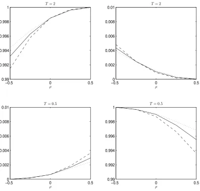
C_finB(ρ)/C_perpB (ρ) and C_finT (ρ)/C_vanillaT (ρ) as functions ofρ in these two limiting cases. We use the Heston model with κ= 2, θ= 0.09 and η = 0.250. We use 5 values of ρ: ₋0.5,₋0.25, 0, 0.25 and 0.5. We let V0 = B = 0.087, implying a µ(B) of about 1 year. We use two values

ofT, 0.5 years and 2 years, corresponding to two cases: T is relatively smaller thanµ(B), and

T is relatively larger than µ(B). All four quantities needed in these two ratios are computed through Monte Carlo simulation. We use 4 million sample paths with a time step of two hours. The results are plotted in Figure 1. The two left subplots are the probabilities ˆEρ₀[1_τB_<T] for

T = 2 years and T = 0.5 years, respectively. The two right subplots are the probabilities ˇ

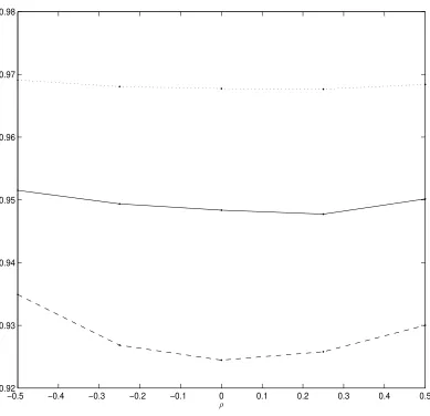
Eρ₀[1ξT<B] for T = 2 years and T = 0.5 years, respectively. The three curves in each subplot correspond to three different values of the strike price K: 90 (dotted line), 100 (solid line), and 110 (dashed line). Monte Carlo simulation is performed to compute these probabilities. We see that these probabilities have weak ρ dependence when the difference of T and µ(B) are relatively large.

The above analysis shows that when the difference of T and µ(B) is reasonably large, the following is a good approximation

Cfin(ρ)≈CperpB (ρ)

C_finB(0)

CB perp(0)

+C_vanillaT (ρ) C

T fin(0)

CT vanilla(0)

. (85)

By design, in the limits ofT _≪µ(B) orT _≫µ(B), this approximation approaches the correct corresponding limits and becomes exact.

The approximation in Equation (85) turns out to be accurate even whenT andµ(B) are of comparable magnitude. This might be at first sight very surprising, because the probabilities ˆ

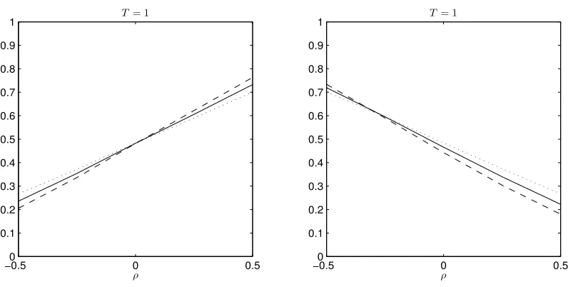
Eρ₀[1_τB_<T] and ˇEρ₀[1_ξT<B] have very strongρ dependence individually in this case, as depicted by Figure 2, which plots the two probabilities ˆEρ₀[1_τB_<T] and ˇEρ

0[1ξT<B] again, but this time withT = 1 year. We see that ˆEρ₀[1_τB_<T] changes from 0.27 to 0.70 as we varyρ from−0.5 to 0.5. Similarly, ˇEρ₀[1ξT<B] changes from 0.70 to 0.27 in this range of ρ.

the perpetual timer option is exercised at a fixed time µ(B), and is therefore equivalent to a plain-vanilla option. In turn, if η is small, for anyρ and any B, we have

C_perpB (ρ)_≈C_vanillaµ(B) (ρ). (86)

Comparing Equations (85) and (80), we see that in this case, in order for the approximation to work well, we do not need the individual probabilities to have weak dependence onρ. Rather, whenCB

perp(ρ)≈CvanillaT (ρ) or equivalentlyT ≈µ(B), as long as the sum

ˆ

Eρ₀[1_τB_<T] + ˇEρ₀[1_ξT<B] (87)

has weak dependence onρ, the approximation in Equation (85) would be very accurate because of Equation (86). Essentially, whenT _≈µ(B), the plain-vanilla option price and the perpetual timer option price are very close, and as long as the sum of the two probabilities is relatively constant as a function of ρ, it does not matter what value we assign to each of the two probabilities.

Unfortunately, it is theoretically very challenging to analyze the sum of these two proba-bilities under generalρ. Notice that the probabilities are taken under two different measures

ˆ

Qρ and ˇQρ. These two measures are related to the risk-neutral measure Q through the two Radon-Nikodym derivatives defined earlier. We caution that even in the special case ρ = 0, the measures ˆQ0, ˇQ0 andQare still all different. To establish the weak dependence of the sum in Equation (87) on ρ when T _≈µ(B), we resort to Monte Carlo analysis again. We still use the Heston model with the same parameters, and plot the sum in Equation (87) as a function ofρ forT = 1 year. The result in Figure 3 clearly shows the weak dependence of the sum on

ρ whenT _≈µ(B).

In view of this analysis, the approximation in Equation (85) should not be thought of as simply freezing the individual probabilities ˆEρ₀[1_τB_<T] and ˇEρ

0[1ξT<B] at their corresponding

ρ = 0 values. Rather, it is crucial that we replace these two probabilities with their ρ = 0 counterpartssimultaneously. WhenT is comparable toµ(B), the bias induced by overestimat-ing one of the two probabilities is offset to a great extend by the underestimatoverestimat-ing of the other probability. In summary, the accuracy of the approximation is safeguarded by the fact that it is exact in the limitsT _≪µ(B) andT _≫µ(B), and that sum in Equation (87) is stable when

T _≈µ(B). Since both sides of Equation (85) are smooth functions ofT, it is understandable that the approximation should be accurate for other values ofT, by continuity.

We assume that C_vanillaT (ρ) can be readily computed in closed form or by methods such as analytical approximation, Fourier inversion, etc. The quantities C_finB(0) and C_finT (0) can be computed by Proposition 3. The perpetual pricesCB

perp(ρ) andCperpB (0) can be computed very

reliably using the approximations in Li and Mercurio (2013). We remark also that the weights

The finite-maturity timer puts under nonzeroρ can be approximated in a similar fashion:

Pfin(ρ)≈PperpB (ρ)

P_finB(0)

PB perp(0)

+P_vanillaT (ρ) P

T fin(0)

PT vanilla(0)

. (88)

Besides being accurate forT _≫µ(B),T _≪µ(B), andT _≈µ(B), the above approximations are exact when ρ = 0 by construction. They are also trivially exact when η = 0 because in this case, ρ is irrelevant for the pricing of both finite-maturity and perpetual timer options, as well as plain-vanilla options. Therefore, by continuity, the approximation should also be reasonably accurate for small η.

In actual implementation, the above matched asymptotics approximation contains two sources of errors. One error is the intrinsic error due to the approximation by matching theρ

behavior asymptotically for T _≪ µ(B) and T _≫ µ(B). The other error comes from approx-imating the quantities involved in the equations. In the Heston model, since the perpetual price approximation in Li and Mercurio (2013) is very accurate, and the vanilla prices can be computed very accurately using Fourier inversion, the main source of error is the compu-tation of CB

fin and CfinT , or PfinB and PfinT. As we have commented earlier, these quantities are

relatively inaccurate compared to other quantities due to the fact that the quantile FξT(B) is not as accurately approximated. If the weights can be computed accurately, the above ap-proximation should be very accurate when the maximum maturity is much larger than the target exercise time implied by the variance budget, or vice versa. The matched asymptotic correlation behavior safeguards the cases with medium maximum maturity values. As we will see in the numerical analysis below that despite of the simplicity, this matched asymptotic approximation is reasonably accurate.

2.5

A Comparison of Different Analytic Methods

Now that we have derived the approximation for the finite-maturity timer option price, we make some comparison with other direct analytic methods. This will allow us to see more clearly the advantages of the proposed method over other methods, as well as its limitations. At first glance, it seems that the finite-maturity timer option price can be obtained through the knowledge of the joint moment generating function of (VT, ξT), which is known in some

models such as the Heston model. This is unfortunately not the case. While this joint dis-tribution is useful for obtaining European-style option prices because of fixed maturity T, for perpetual timer options we need the joint distribution ofτB _and ∫τB

0

√

VudWuV, where τB is

the random time for ξt to hit B.5 For finite-maturity timer options, we need the joint

dis-tributions of τ and ∫₀τ√VudWuV, where τ = min(τB, T). This is a completely new problem

5

from the joint distribution of (VT, ξT) and is mathematically very challenging, even for the

perpetual timer option case.

As far as we know, the only model in which the joint distribution ofτB _and∫τB 0

√

VudWuV

has been worked out explicitly is the Heston model (see C.X. Li (2013)). The Heston model is very special since in this model∫₀τB√VudWuV can be expressed as a simple linear function

of V_τB and τB. C.X. Li (2013) utilizes a time-change technique and relies crucially on known results for Bessel processes. The joint density of τB and V_τB is given by a complex Laplace inverse transformation in Proposition 3 of C.X. Li (2013), where the integrand involves modified Bessel functions with complex arguments. Special attention needs to be paid to the winding of the Bessel argument. The final pricing formula in Equation (5.3) of their paper is also fairly complicated. We emphasize again that the method only works for the Heston model and perpetual timer options. The author also only considers the zero dividend case. Nonzero dividend makes the analysis more complicated because the combination S_τBe−δτ

B

appears after we condition on the filtration generated byVu. This combination involves two correlated

random variables, which increases complexity of the analysis. This situation differs from the European-style plain-vanilla options case, where it is easy to take into account a nonzero dividend rate because there e−δT _{is just a deterministic number.}

To our knowledge, the only other analytic method that has been proposed for finite-maturitytimer option prices under nonzero interest rate besides the current paper is Liang et al (2011). This paper utilizes the known results on path integrals of the Morse and Kratzer potentials in quantum field theory to study the Heston and 3/2 models. The method works for both perpetual and finite-maturity timer options. The authors only consider the zero dividend case. The math is extremely difficult. The handling of finite-maturity feature in Liang et al (2011) is highly nontrivial and requires the ability to Fourier inverse transform the marginal propagator of the stock price (Equation (35) in their paper).

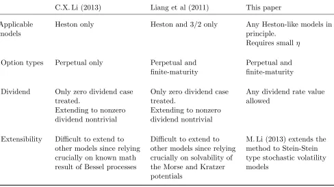
In Table 1, we summarize the applicability of the three methods: C.X. Li (2013), Liang et al (2011), and the method in this paper. While C.X. Li (2013) only deals with perpetual timer options and technically is not a competitor of our approximation method, we include it because it is closely related. We notice that our method is the only method that can be applied to nonzero dividend case without any additional effort, and the only method that can be applied to models beyond the Heston model or the 3/2 model.6 In this sense, rather than being competitors, our method and the methods in C.X. Li (2013) and Liang et al (2011) are complementary to each other. The limitation of our method is also clear: it is an approximation derived under the assumption of a small eta in the diffusion function. It is an empirical question

6

as to how small the parameter eta needs to be in individual models, and numerical analysis needs to be carried out for any production level implementation.

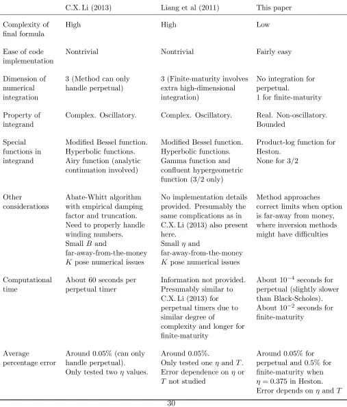
In Table 2, we compare the implementation aspects of the three methods, as well as their performance. While it is highly nontrivial to implement both C.X. Li (2013) and Liang et al (2011), it is fairly easy to implement our approximation method. The complications in the former two methods include: high-dimensional numerical integration, integration in complex plane where one needs to pay special attention to branch cuts and poles, oscillatory integrand which can potentially be slowly decaying, and the involvement of special functions such as modified Bessel function, Airy function, gamma function, and confluent hypergeometric func-tion. As for performance, the method in C.X. Li (2013) requires about 60 seconds to price one perpetual timer option with a percentage of about 0.05%. Due to the high dimension of integration involved, to reach higher accuracy would require considerably more time. No information on speed is provided in Liang et al (2011), but it is conceivable that it would take somewhat longer time because of the added complexity to handle the finite-maturity feature. To contrast, the approximation method in Li and Mercurio (2013) takes about 10−4 _seconds

for perpetual timer options and in this paper the method takes about 10−2 _{seconds for a}

finite-maturity option.7 _{In terms of accuracy, both C.X. Li (2013) and Liang et al (2011) report an}

average percentage error of about 0.05%. These papers only test a few parameter values and do not systematically study the error as a function ofT orη. The errors of our approximation will be reported in more detail in the numerical analysis section. The average percentage error for finite-maturity option prices is about 0.5%. The error becomes considerably smaller when

η is small or whenT is large compared toµ(B).

One additional attractive property of our method manifests itself when we need to value a far-way-from-the-money timer option for which the strikeK is much smaller or much larger than the current stock priceS0. It is well-known that the usual Fourier inversion for

European-style options becomes inaccurate numerically due to the oscillatory integrand. It is conceivable that similar difficulty will also arise in the timer option case with complex inversion methods. To contrast, when dividend rate is zero, our approximation approaches the correct no-arbitrage limit prices whenK _→0 orK _{→ ∞}, therefore providing robustness for the method.

3

Numerical Analysis

Below we examine the accuracy of our pricing approximation numerically. We do this by first looking at the performance for the zero correlation case, and then for the nonzero correlation

7_{The approximation method has an additional attractive property in thatµ(B) and σ(B) do not depend onK,}

case. For both cases, we examine the performance for both timer calls and puts.

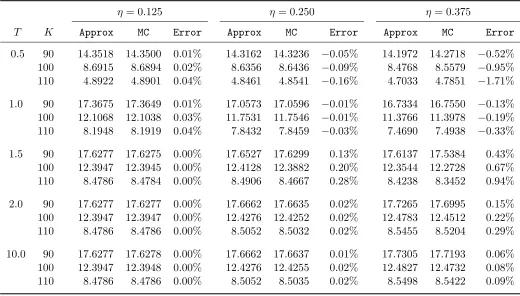
Table 3 reports the performance of our approximation for timer call options under the Heston model with zero correlation. Parameters used here are the same ones as in Liang, Lemmens and Tempere (2011): V0 = 0.087, κ= 2, θ= 0.09, r = 0.015, S0 = 100, andδ = 0.

The variance budgetBequalsV0, implying a target exercise maturity of about 1 year. We vary

the value of the maximum maturityT to be 0.5, 1.0, 1.5, 2.0, and 10 years, and volatility of variance coefficientη to be either 0.125, 0.250, or 0.375, ranging from small to relatively large. Monte Carlo prices are simulated based on Proposition 2 using 4,000,000 sample paths with a time step of every 2 hours and the terminal accumulated variance as the control variate. The unreported standard errors from simulation are all in the order of 10−4_{or smaller. Each Monte}

Carlo simulation takes about 20 to 40 minutes for the desired accuracy. The approximated prices are computed using Proposition 3 with the quantitiesµ(B) andσ(B) given in Example 1. The percentage errors are computed using the Monte Carlo prices as benchmarks.

With the given parameters, when η = 0.125, the random budget exceeding time τB is approximately normally distributed with µ = 0. .9969 and σ = 0. .1255. When η = 0.250, we have µ = 1. .0445 and σ = 0. .2510. When η = 0.375, we have µ = 1. .1239 and σ = 0. .3765. The range of maximum maturities we use therefore covers situations where the cutoff is very stringent to where it is very loose. In terms of the timer call price decomposition, the relative magnitude ofC_finB and C_finT therefore ranges from very small to very large. This wide range of

T allows us to look at the accuracy of our approximation more comprehensively.

As we see in Table 3, our approximation is fairly accurate in general. For the relatively small value of η = 0.125, our approximation is extremely accurate, with percentage errors all in the order of 0.01%. We also see that a maximum maturity of 2 years or more puts effectively no constraint on the timer option. The approximation is still very accurate for the medium value of η= 0.250. The relatively large percentage errors occur when η is large and the maximum maturity is stringent, that is, whenη= 0.375 andT <2.0. Whenη= 0.375 but the maximum maturity is less stringent, we see that the percentage errors get much smaller. We also remark that in practice, when a timer option contract is first initiated, the maximum maturity is usually fairly loose, with typical maximum maturity 3 or 6 times the target exercise maturity. However, a timer option on an existing trade book could have a stringent maximum maturity cutoff as time progresses.

a large volatility gives more optionality to exercise the option, but also increases the risk that the option becomes knocked-out.

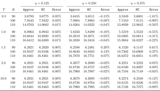
Table 4 reports the performance of our approximation for timer put options under zero correlation. The parameters used are exactly the same ones as in Table 3. In contrast to Table 3, Table 4 shows that the timer put prices are all decreasing inηregardless of the values of T and K. The general patterns of pricing errors are the same as in Table 3 so we do not discuss the details here. The approximation is again extremely accurate when the maximum maturity cutoff is less stringent, and whenη is not large.

One question is whether the accuracy of our approximation is due to the particular pa-rameter vector we have used. In unreported analysis, we have performed extensive sensitivity analysis. The following is a partial set of what we have done.

1. We change the interest rater to be either 0 or 3%.

2. We change the value of B to be twice of or half of the value we use right now.

3. We change the value of V0 to be either 25% or 4 times the value we use right now.

4. We examine a much wide range of strikes, from K= 50 toK = 150.

In virtually all those cases, the accuracy of our approximation in terms of percentage errors remains the same. The only exception is when the option is deeply out-of-the-money, so the percentage error gets large, but the absolute error is still small. That the approximation works for a wide range of strikes makes it more useful in real applications.

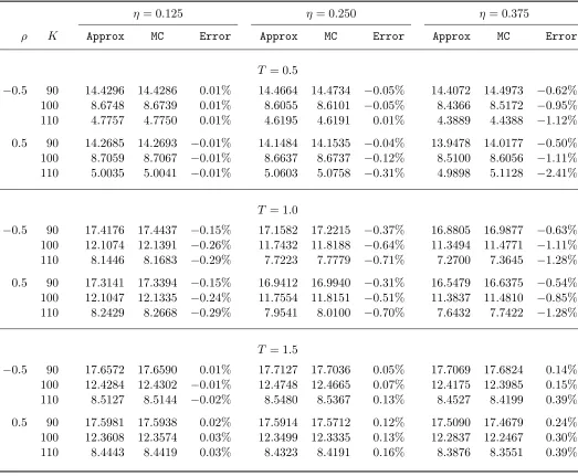
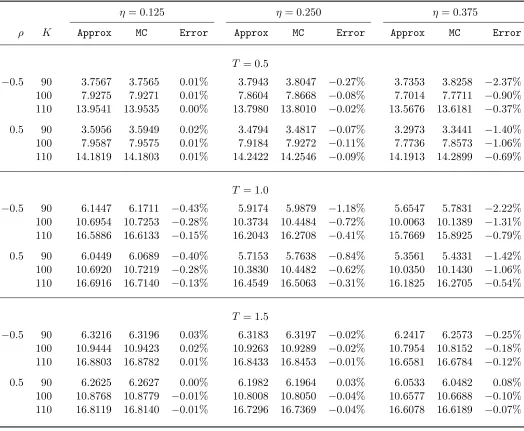
Tables 5 and 6 report the performance of our approximation under the Heston model with nonzero correlation for finite-maturity timer call and put options, respectively. The parameters used are still the same ones as in Liang, Lemmens and Tempere (2011). Same as in Liang, Lemmens and Tempere (2011), we consider two values of nonzeroρ, namely₋0.5 and 0.5. We consider three values ofT: 0.5, 1.0, and 1.5 years. The maturities T are chosen to cover the three cases that T is smaller than, roughly equal to, and larger than the target exercise time implied byB. Again, three values of η are considered, ranging from small to relatively large. The benchmark prices are obtained from Monte Carlo using Equation (73) with 4,000,000 sample paths and a time step of every 2 hours. Not surprisingly, with nonzeroρ, the accuracy of Monte Carlo decreases. However, the results are still very accurate, with standard errors all in the order of 10−3 _{or smaller.}

approximation in general follows the Monte Carlo prices closely and also exhibits those complex

η dependencies.

In both Tables 5 and 6, we see that our simple approximation is fairly accurate, especially when η is small, or when T is large. We see that for all entries with η = 0.125 or T = 1.5, the percentage errors are all smaller than ₋0.50% for both calls and puts. For η = 0.250, we see that the errors are larger for T = 1.0, where the constraints due to T and B are of comparable magnitudes. The accuracy decreases significantly for η = 0.375. One reason is thatC_finB and C_finT needed in the approximation become less accurate for largeη. For example, in Table 5, whenρ= 0.5 andη= 0.375, the percentage errors for the three different strikes are

−0.50%,₋1.11%, and₋2.41%. Had we used the values ofC_finB andC_finT from Monte Carlo, the three errors would have been ₋0.01%, ₋0.06%, and ₋0.19%. This suggests that if accurate values ofCB

finandCfinT are available through other means, then the performance of the matched

asymptotic approximation can be improved, especially for relatively small or relatively largeT.

4

Conclusion

In this paper, we develop an approximation for pricing finite-maturity timer options under general stochastic volatility models. The method works for both timer calls and timer puts. For zero correlation between the Brownian motions, we use the results in M. Li (2013) to approximate the probability densities we need and obtain analytic expressions for the timer option prices. For nonzero correlation, we use a linear combination approximation which matches the asymptotic correlation behavior when the maximum maturity is much larger than the target exercise time implied by the variance budget, or vice versa.

Numerical study using the Heston model shows that the approximate timer option prices under zero and nonzero correlations are fairly accurate. The approximation is more accurate when the volatility of variance is small or when the maximum expiry is not tightly binding.

References

Ahn, D.H., and B. Gao. 1999. A parametric nonlinear model of term structure dynamics.

Review of Financial Studies12, 721–762.

Bernard, C., Z. Cui. 2011. Pricing timer options. Journal of Computational Finance 15(1), 69–104.

Bick, A. 1995. Quadratic-variation-based dynamic strategies.Management Science41(4), 722– 732.

Carr, P., and R. Lee. 2010. Hedging variance option on continuous semimartingales.Finance and Stochastic 14, 179–207.

Folland, G.B. 1999. Real Analysis: Modern Techniques and Their Applications. Wiley.

Hawkins, D., and S. Krol. 2008. Product overview: Timer options. Lehman brothers Equity Derivatives note.

Heston, S.L. 1993. A closed-form solution for options with stochastic volatility with applica-tions to bond and currency opapplica-tions.Review of Financial Studies6(2), 327-343.

Hull, J., and A. White. 1987. The pricing of options on assets with stochastic volatilities.

Journal of Finance 42(2), 281–300.

Lee, R. 2012. Timer options for risk-controlled variance exposure. Global Derivatives USA 2012 conference presentation.

Lewis, A.L. 2000. Option Valuation Under Stochastic Volatility. Finance Press, Newport Beach, California.

Li, C.X. 2010. Managing volatility risk. Doctoral Dissertation, Columbia University.

Li, C.X. 2013. Bessel processes, stochastic volatility, and timer options.Mathematical Finance, forthcoming. DOI:10.1111/mafi.12041

Li, M. 2013. Derivatives pricing on integrated diffusion processes: A general perturbation approach. Working paper. Bloomberg LP.

Li, M., F. Mercurio. 2013a. Closed-form approximation of timer option prices under general stochastic volatility models. Working paper. Bloomberg LP.

Liang, L.Z.J., D. Lemmens, and J. Tempere. 2011. Path integral approach to the pricing of timer options with the Duru-Kleinert time transformation.Physical Review E(83).

Lipton, A. 2001. Mathematical Methods for Foreign Exchange: a Financial Engineers Ap-proach. World Scientific.

Neuberger, A. 1990. Option pricing: A non-stochastic approach. Working paper. London Busi-ness School.

Romano, M., and N. Touzi. 1997. Contingent claims and market completeness in a stochastic volatility model.Mathematical Finance 7(4), 399–412.

Royden, H. 1988. Real Analysis. Pearson.

Saunders, D. 2010. Pricing timer options under fast mean-reverting stochastic volatility. Work-ing paper.

Sawyer, N. 2007. SG CIB launches timer options.Risk20(7), 6.

Sawyer, N. 2008. Equity derivative house of the year: Soci´et´e G´en´erale.Risk 21(1).

Toft, K.B. 1996. On the mean-variance tradeoff in option replication with transactions costs.

Table 1: Applicability of Different Analytic Methods

C.X. Li (2013) Liang et al (2011) This paper

Applicable models

Heston only Heston and 3/2 only Any Heston-like models in principle.

Requires smallη

Option types Perpetual only Perpetual and finite-maturity

Perpetual and finite-maturity

Dividend Only zero dividend case treated.

Extending to nonzero dividend nontrivial

Only zero dividend case treated.

Extending to nonzero dividend nontrivial

Any dividend rate value allowed

Extensibility Difficult to extend to other models since relying crucially on known math result of Bessel processes

Difficult to extend to other models since relying crucially on solvability of the Morse and Kratzer potentials