Soil Thermal Diffusivity of a Gleyic Solonetz Soil
Estimated by Different Methods in the
Brazilian Pantanal
Victor H. M. Danelichen1, Marcelo S. Biudes1, Maísa C. Souza1, Nadja G. Machado1,2, Leone F. A. Curado1, José S. Nogueira1
1Postgraduate Program in Environmental Physics, Physics Institute, Federal University of Mato Grosso (UFMT), Cuiaba, Brazil; 2Laboratory of Conservation Biology, Federal Institute of Mato Grosso, Cuiaba, Brazil.
Email: [email protected], [email protected], [email protected], [email protected], [email protected]
Received December 4th, 2012; revised January 8th, 2013; accepted January 20th, 2013
ABSTRACT
The soil temperature is an important microclimatic factor due to the interactions between soil and plant, and the energy exchange with the atmosphere. The soil energy exchange is affected by the incident solar radiation, type of coverage and mainly by the soil thermal properties. Among the soil thermal properties, the soil thermal diffusivity is highlighted because it affects the soil temperature profile and soil heat flux transport and distribution. Thus, the aim of this study was to evaluate different estimates of soil thermal diffusivity of a Gleyic Solonetz soil in the Brazilian Pantanal. The soil thermal diffusivity was determined by the amplitude, logarithmic, arctangent and the phase methods between 0.01 and 0.03 m, 0.01 and 0.07 m and 0.01 and 0.15 m depth. The soil thermal diffusivity estimated by the four methods showed significant differences and varied over the study period as a function of volumetric soil water content. The soil thermal diffusivity estimated by logarithmic methodshowed better performance at different depths, followed by the method of phase.
Keywords: Water Content; MonodominantForest; Soil Thermal Properties; Soil Temperature Profile
1. Introduction
Brazilian Pantanal is one of the largest floodplains of the Earth with 138,183 km2, and 35% of its area is in Mato Grosso state. Paraguay River crosses the Pantanal from North to South and becomes larger and formsa complex river system [1]. The climate is characterized by periods of floods and droughts that alternate throughout the year, allowing the formation of monodominants stands. At the other extreme, frequent drought cause local water stress in plants which regulates its phenology and mass produc- tion [2].
The soil temperature is a factor which controls micro- climatic seed germination, rate and duration of plant growth and development, nutrient uptake, water and gas distribution in soil as well as the growth and develop- ment of microorganisms [3]. Considering each soil type has unique characteristics, it is necessary to identify, for each particular situation, their thermal properties, which are the result of a number of factors, including its texture and chemical composition. Regular observations of soil temperature at different depths allow the knowledge of
their thermal profile variation and important soil proper- ties such as soil thermal conductivity and soil thermal diffusivity [4]. These soil thermal properties, especially the soil thermal diffusivity, are used in studies of soil temperature simulation at different depths [5].
Soil thermal diffusivity is an important parameter that affects soil temperature distribution and soil heat flux density [6]. Furthermore, it is a property that informs the soil heating speed that relate with soil thermal conducti- vity and soil thermal capacity [7].
The estimation of soil thermal diffusivity can be de-termined by various methods, such as amplitude, phase, arctangent, logarithmic, numeric and harmonic, which utilize soil profile temperature measurements [8]. These methods are based on the soil heat transfer theory, using analytical or numerical solutions of the heat conduction equation described as uniform and homogeneous soil [5].
2. Materials and Methods
2.1. Characterization of the Study Area
The experiment was conducted in an experimental area of Reserva Particular do Patrimônio Natural-RPPN SESC Pantanal (16˚39'50''S; 56˚47'50''W; 120 m of alti- tude) in the Barão de Melgaço, Mato Grosso, Brazil be- tween October 2008 to February 2009, during the period when there was no flooding, which occurred in March 2009. This area is composed mainly of Vochysiadiver- gens Pohl, known locally as cambarazal, with 28 - 30 m canopy heights, forming a continuous band of approxi- mately 25 km long and 4 km wide, parallel to the Cuia- báriver. The annual average temperature is between 24.9˚C to 25.4˚C, annual rainfall is on average 1400 mm with a pronounced dry season extending from May through September [9]. The topography of the floodplain is virtually flat, causing extensive flooding during the wet season. Wet-season floods are 1 to 2 m in depth, but during the dry season many of the floodplain lakes be- come disconnected from the river channel as the flood- water recedes [10]. The soil type of the study site is clas- sified as a Gleyic Solonetz soil [11].
2.2. Instrumentation
Precipitation data were obtained daily by personnel of RPPN SESC-Pantanal from a manual rainfall gauge lo- cated 10 km NW of experimental area. Soil temperature was measured at 1, 3, 7, 15 and 30 cm depth, using five thermistors (108-L, Campbell Scientific, Inc., Logan, Utah, USA). These depths were chosen due the higher soil temperature amplitude from surface to 7 cm depth and practically null at 30 cm depth. Volumetric soil wa- ter content was measured with two time domain reflec- tometer (CS-615, Campbell Scientific, Inc., Logan, Utah, USA) at 5 and 25 cm depth. The sensors which produced signals that were stored by a datalogger (model CR10-X; Campbell Scientific, Logan, UT).
2.3. Estimation of Soil Thermal Diffusivity The one-dimensional heat conduction in soil is given by Equation (1).
T
C CK
t z z
T
(1)
where T is the soil temperature, t is the time and z is the depth. Due to the partitioning of a not uniform soil in soil layers with uniform composition and texture, the Equa- tion (1) can be rewritten to Equation (2).
2 2 j T K t z T
(2)
where Kj =(k/C)j is the apparent soil thermal diffusivity of j layer, delineated by zj − 1 and zj + 1, with j = 1, 2,···,
m the number of layers, not necessarily same thicknesses. The apparent soil thermal diffusivity can be obtained by the soil temperature measurements replaced in ex- pression of analytical solutions of Equation (2). Several methods have been used to solving this Equation [12]. In this study the soil thermal diffusivity was estimated be- tween 0.01 and 0.03 m, 0.01 and 0.07 m and 0.01 and 0.15 m depth by the amplitude, logarithmic, phase and arctangent methods.
2.3.1. Amplitude Method
The daily soil thermal diffusivity K estimated by ampli- tude method [12] is shown in Equation (3).
2 2 1 1 2 2 ln Z Z K A A (3)where is the angular velocity of the Earth and A1 and A2 are the temperature amplitudes in the Z1and Z2 depths, respectively.
2.3.2. Phase Method
The daily estimation of soil thermal diffusivity by the phase method was obtained by the Equation (4).
2 2 1 1 2 Z Z K t
(4)
where Z1 and Z2 are the soil depths and Δt= t2 −t1, where Δt is the time interval between t1and t2, which are the instant when the temperature is maximum in Z1and Z2.
2.3.3. Arctangent Method
The soil temperature at the surface can be described by a sines series. The values of soil temperature measured at a specific depth can be adjusted to Fourier series [13], given by Equation (5).
1 cos sin M n n nT t T A n t B n t
(5)where T is the average temperature in considered time interval, M is the number of harmonics, An and Bn are their amplitudes, n is the number of observations, is the angular frequency and t is the time. If the first two harmonics are sufficient to describe one boundary condi- tion above the level Z=Z1 (Z1 = 0, the surface level), K can be calculated using Equation (6) of the arctangent method.
2 2 1 21 3 2 4 2 4 1 3
1 3 1 3 2 4 2 4
2 arctan
Z Z
K
T T T T T T T T
T T T T T T T T
where T1, T2, T3 and T4 are the soil temperatures recorded in Z1and T’1, T’2, T’3 and T’4 are the soil temperatures recorded in Z2, at 0, 6, 12 and 18 hours [14].
2.3.4. Logarithmic Method
Using the same methodology of arctangent method, See- mann [15] demonstrated that K can also be calculated by Equation (7).
2 2 1 2 2 21 3 4
2 2
1 3 2 4
0.121
ln
Z Z
K
T T T T
T T T T
(7)
The arctangent and logarithmic methods are analogous to the Amplitude method, but require a greater number of observations to approximate the behavior essentially non-sinusoidal [4].
2.4. Statistical Analysis
The soil thermal diffusivity values using the arctangent, logarithmic and phase methods were compared with the values obtained by the amplitude method. To evaluate these methods, we considered the mean absolute error (MAE; Equation (8)) and root mean squared error (RMSE; Equation (9)).The MAE indicates the distance (deviation) of the mean absolute values estimated from the measured values. Ideally, the MAE and RMSE values were near to zero [16].
MAE Pi Oi n
(8)The RMSE indicates how the model fails to estimate the measurements variability around the mean and meas- ures the change in the estimated values around the meas- ured values [16]. The lower limit of RMSE is 0, which means that there is full compliance between the model estimates and measurements.
2RMSE Pi Oi n
(9)where Pi is the estimated value, Oiis the observed value and O is the average of the observed values.The multi- variate analysis of variance test-MANOVA was used to determine possible differences between the methods for estimating the soil thermal diffusivity.
3. Results and Discussion
3.1. Variation in Rainfall, Volumetric Soil Water Content and Soil Temperature
The monthly rainfall was 138, 121, 320, 105 and 305 mm
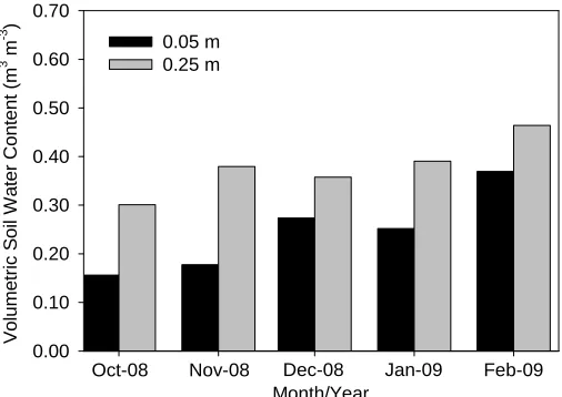
in October, November and December 2008, and January and February 2009, and the total accumulate drain fall was 989 mm during the study period (Figure 1). The volumetric soil water content (VSWC) increased from October 2008 to February 2009 (Figure 2) as a function of increased local rainfall (Figure 1). The largest amount of VSWC coincides with the wettest month, and the in- verse occurs with the driest month. The highest VSWC occurred during February 2009, with 0.38 and 0.47 m3·m−3 at 0.25 to 0.05 m depth, and the lowest VSWC occurred during October 2008, with 0.15 and 0.30 m3·m−3 at 0.25 to 0.05 m depth (
Figure 3).
The average maximum soil temperature decreased from October to December, while the minimum soil tem- perature had less variation. The maximum soil tempera- tures increased from January to February 2009, but at a lower rate than October-December 2008, and also the minimum soil temperature values increased from January to February 2009 (Figure 2). The average maximum soil temperatures at 0.01 m depth were 32.8˚C, 31.3˚C, 29.6, 29.9˚C and 30.9˚C at 13 h, 13 h and 30 min, 15 h, 15 h and 15 h and 30 min in October, November and Decem- ber 2008 and January and February 2009, respectively. The average minimum soil temperatures at 0.01 m depth were 24.0˚C, 24.1˚C, 23.9˚C, 23.7˚C and 25.1˚C at 6 h, 5 h and 30 min, 30 min and 5 h, 6 h and 6 h and 30 min in October, November and December 2008 and January and February 2009, respectively. The attenuation of the maximum soil temperature from 0.01 m to 0.30 m depth was 6.1˚C, 4.4˚C, 2.8˚C, 3.3˚C and 4.0˚C with a lag of 11 h 30 min, 10 h, 9 h 30 min, 9 h and 10 h in October, No- vember and December 2008 and January and February 2009, respectively.
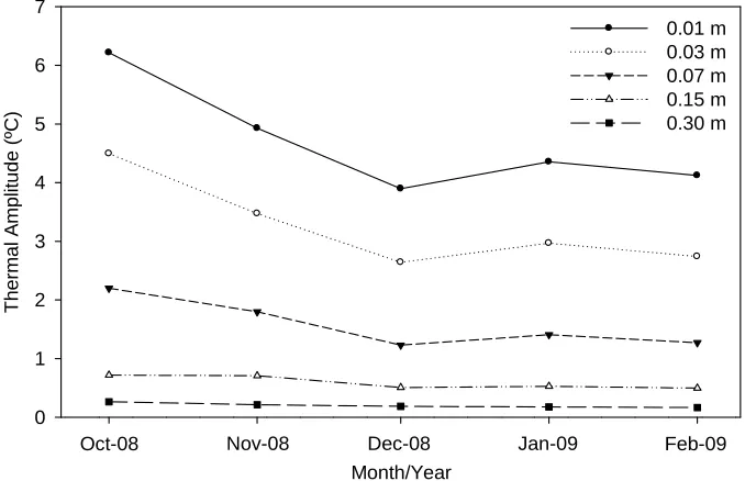
The soil temperature amplitude decreased from Octo- ber to February (Figure 4), reflecting the increase of water content in soil, caused by increased rainfall over the period (Figure 3). The soil temperature amplitude reduction during the summer, during this work, is due the higher VSWC (Figure 3) that changes the magnitude of energy balance components, and modify the properties of soil heat conduction [17,18]. The water fills the soil pores, which contribute to increase heat flux and de- crease soil temperature amplitude [19].
[image:3.595.91.288.182.268.2]Month/Year
Ra
in
fa
ll (
m
m mon
th
-1 )
0 50 100 150 200 250 300 350 400
[image:4.595.168.428.89.277.2]Oct-08 Nov-08 Dec-08 Jan-09 Feb-09
Figure 1. Monthly rainfall in the Brazilian Pantanal from October 2008 to February 2009.
06 12 18 06 12 18 06 12 18 06 12 18 06 12 18
00 00 00 00 00 00
S
o
il T
e
mperat
ure
(º
C)
24 26 28 30 32 34
0.01 m 0.03 m 0.07 m 0.15 m 0.30 m
[image:4.595.166.430.310.485.2]Out-08 Nov-08 Dec-08 Jan-09 Feb-08
Figure 2. Mean monthly composite average of the diel soil temperature at 0.01, 0.03, 0.07, 0.15 and 0.30 m depth in the Bra-zilian Pantanalfrom October 2008 to February 2009.
Month/Year
V
o
lume
tric S
o
il
W
a
te
r C
ont
ent
(m
3 m
-3 )
0.00 0.10 0.20 0.30 0.40 0.50 0.60 0.70
0.05 m 0.25 m
Oct-08 Nov-08 Dec-08 Jan-09 Feb-09
[image:4.595.171.424.526.705.2]Month/Year
Thermal A
m
plitude
(ºC)
0 1 2 3 4 5 6 7
0.01 m 0.03 m 0.07 m 0.15 m 0.30 m
[image:5.595.127.466.89.308.2]Oct-08 Nov-08 Dec-08 Jan-09 Feb-09
Figure 4. Mean monthly soil temperature amplitude at 0.01, 0.03, 0.07, 0.15 and 0.30 m depth in the Brazilian Pantanal from October 2008 to February 2009.
soil is assumed that there is higher VSWC and it alters the soil specific heat and soil thermal conductivity. Thus, the soil heat capacity increases with VSWC increases due to the high water specific heat (4.18 MJm−3·K−1) [7].
3.2. Variation of Soil Thermal Diffusivity
The highest average of soil thermal diffusivity estimated by the amplitude method was 1.95 × 10⁻⁷ m2·s−1 in No- vember 2008between 0.01 and 0.15 m depth, and the lowest average was 1.02 × 10⁻⁷ m2·s−1 in December 2008 between 0.01 and 0.03 m depth (Figure 5(a)).The soil thermal diffusivity estimated by amplitude method is used as reference among all used models [5,20]. The soil thermal diffusivity values calculated in this study agreeto estimates by Oliveira etal. [21] in Campina Grande (1.5 − 3.33 × 10⁻⁷ m2·s−1), Souza
etal. [22] in forest and pas- ture in Amazon (1.45 − 6.74 × 10⁻⁷ m2·s−1)and Rao
etal. [4] in Salvador (4.7 − 7.5 10 × 10−7 m2·s−1).
The soil thermal diffusivity estimated by the amplitude method between 0.01 and 0.15 m depth was higher than soil thermal diffusivity between 0.01 and 0.03 and be- tween 0.01 and 0.07 (Figure 5(a)). There was a tendency of increasing of the soil thermal diffusivity estimated by amplitude method as function of increasing of depth. Furthermore, the VSWC seems to be the main factor to regulate the soil thermal diffusivity because the average of VSWC during the studied period was 0.24 m3·m−3 at 0.05 m depth and 0.37 m3·m−3 at 0.25 m depth.
The highest average of soil thermal diffusivity esti- mated by the logarithmic method was 2.47 × 10⁻⁷ m2·s−1 in December 2008 between 0.01 and 0.03 m depth, and the
lowest average was 1.87 × 10⁻⁷ m2·s−1 in January 2009 between 0.01 and 0.07 m depth (Figure 5(d)). The soil thermal diffusivity estimated by the logarithmic method also showed a tendency of increasing as function of in- creasing of depth, with higher values of soil thermal dif- fusivity estimated by amplitude method.
The soil thermal diffusivity estimated by phase (Fi- ure 5(b)) and arctangent(Figure 5(c)) methods showed similar dynamic, with decreasing from October to De- cember 2008, and increasing from December 2008 to February 2009, and values were overestimated in relation to the amplitude and logarithmic methods (Figures 5(a) and 5(d)). The soil thermal diffusivity estimated by arc- tangent method was higher in October 2008 (5.38 × 10⁻⁷ m2·s−1) when the VSWC was lowest. The soil thermal diffusivity estimated by phase method was higher in January 2009 (3.55 × 10⁻⁷ m2·s−1) when the rainfall was lowest.
The VSWC is an important factor to regulate the thermal process in the soil. The soil thermal diffusivity can be higher or lower as function of VSWC [18,23]. The increasing of VSWC becomes the soil thermal con- ductivity higher, because the water that replaces the air in the soil pores has higher thermal conductivity [24]. There were differences in the structure of each layer of soil studied (Figure 6), which influence in water retention, for example, the clay retains more water than the sand interfering in soil thermal diffusivity variation [20]. There is a maximum value to soil thermal diffusivity at a determined VSWC, while the volumetric heat capacity continues to increase with increasing VSWC [25].
Figure 5. Mean monthly soil thermal diffusivity estimated by the amplitude, phase, logarithmic and arctangent methods be- tween 0.01 and 0.03 m, 0.01 and 0.07 m and 0.01 and 0.15 m in the Brazilian Pantanal from October 2008 to February 2009.
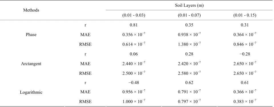
Table 1. Mean absolute error—MAE, root mean squared error—RMSE, Pearson correlation coefficient—r for soil thermal diffusivity estimated by phase, arctangent and logarithmic methods between 0.01 and 0.03 m, 0.01 and 0.07 m and 0.01 and 0.15 m depths, taking as reference values estimated by amplitude method in the Brazilian Pantanal.
Soil Layers (m) Methods
(0.01 - 0.03) (0.01 - 0.07) (0.01 - 0.15)
r 0.81 0.35 0.31
MAE 0.356 × 10⁻⁷ 0.938 × 10⁻⁷ 0.364 × 10⁻⁷
Phase
RMSE 0.614 × 10⁻⁷ 1.380 × 10⁻⁷ 0.846 × 10⁻⁷
r 0.06 0.28 −0.28
MAE 2.440 × 10⁻⁷ 2.420 × 10⁻⁷ 2.650 × 10⁻⁷
Arctangent
RMSE 2.500 × 10⁻⁷ 2.580 × 10⁻⁷ 2.650 × 10⁻⁷
r −0.48 0.62 0.61
MAE 0.956 × 10⁻⁷ 0.791 × 10⁻⁷ 0.366 × 10⁻⁷
Logarithmic
RMSE 1.000 × 10⁻⁷ 0.797 × 10⁻⁷ 0.383 × 10⁻⁷
thermal diffusivity of soil have been made to different locations and specific depths [4,12,22,26,27]. However, they were restricted to describe the soil thermal diffusivi- ty values estimated by the methods studied in this work.
The normality of the soil thermal diffusivity was checked and was applied MANOVA statistical test to evaluate if there were differences between the estimates of soil thermal diffusivity at each depth at 5% probability. The soil thermal diffusivities estimated by the methods of amplitude, phase, and the logarithm of the arctangent differed (p < 0.05) and varied over time (Figure 5).
Using the soil thermal diffusivity estimated by ampli- tude method as reference was computed mean absolute error-MAE and the root mean squared error-RMSE be- tween phase methods, arctangent and logarithmic. Among the three methods the phase method showed lower EMA between 0.01 and 0.03 m depth and the logarithmic method showed lower RMSE between 0.01 to 0.15 m depth. The phase method showed higher correlation (r = 0.81) between 0.01 and 0.03 m depth, followed by loga- rithmic method (r = 0.62) between 0.01 and 0.07 m depth and (r = 0.61) between 0.15 to 0.01 m depth, while the arctangent method showed no significant correlation (Table 1).
4. Conclusions
The soil thermal diffusivity estimated by the four meth- ods showed significant differences (p < 0.05) and varied over the study period as a function of water content in the soil.
Even the methods to estimate soil thermal diffusivity are significant different the methods of phase, logarithm- mic and arctangent were significantly correlated to the amplitude method.
The method of estimation of the soil thermal diffusiv- ity that showed better performance at different depths was the logarithmic method, followed by the phase method with the highest correlation to lowest depth.
The estimation of soil thermal diffusivity by phase method showed lower mean absolute error to less depth, while the logarithmic method showed lower mean squared error to greater depth.
5. Acknowledgements
Thisresearchwassupported in partby Universidade Federal de Mato Grosso (UFMT), Conselho Nacional de Desen- volvimento Científico e Tecnológico(CNPq), andfromlo- gisticalsupportfromtheReserva Particular do Patrimônio Natural (RPPN) ofthe Serviço Social do Comércio (SESC)-Pantanal.The authors thank Vicente Bellaver (in memoriam) for help with field sampling and soil labora-tory analysis.
REFERENCES
[1] M. N. Castelnou, D. Floriani, I. A. Vargas and J. B. Dias, “Sustentabilidade Socioambiental e Diálogo de Saberes: O Pantanal Mato-Grossense e Seu Espaço Vernáculo Co- mo Referência,” Desenvolvimento e Meio Ambiente, Vol.
7, 2003, pp. 41-67.
[2] W. J. Junk and C. N. Cunha, “Pantanal: A Large South American Wetland at a Crossroads,” Ecological Engi- neering, Vol. 24, No. 4, 2005, pp. 391-401.
doi:10.1016/j.ecoleng.2004.11.012
[3] E. Gasparim, P. R. Ricieri, S. S. Lima, R. Dallacort and E. Gnoatto, “Temperatura No Perfil Do Solo Utilizando Duas Densidades de Cobertura e Solo Nu,” Acta Sci- entiarum. Agronomy, Vol. 27, No. 1, 2005, pp. 107-115.
rísticas Termicas do Solo em Salvador, BA.,” Revista Brasileira de Engenharia Agrícola e Ambiental, Vol. 9, No. 4, 2005, pp. 554-559.
doi:10.1590/S1415-43662005000400018
[5] V. H. M. Danelichen and M. S. Biudes, “Avaliação da Difusividade Térmica de um Solo no Norte do Pantanal,”
Ciência e Natura, Vol. 33, No. 8, 2011, pp. 227-240.
[6] C. C. L. Beber, “Difusividade de Solos do Tipo Latossolo Vermelho em Função do Teor de Umidade,” M. Sc. Thesis, Universidade Regional do Noroeste do Estado do Rio Grande do Sul, Ijuí, 2006.
[7] E. R. Schöffel and M. E. G. Mendes, “Influência da Cobertura Sobre o Perfil Vertical de Temperatura do Solo,” XIV Congresso Brasileiro de Agrometeorologia, Piracicaba, 18-21 July 2005, pp. 1-2.
[8] R. Horton, E. O. Tyson and T. Ren, “A New Perspective on Soil Thermal Properties,” Soil Science Society of American Journal, Vol. 65, No. 6, 2001, pp. 1641-1647. doi:10.2136/sssaj2001.1641
[9] M. S. Biudes, J. S. Nogueira, H. J. Dalmagro, N. G. Ma- chado, V. H. M. Danelichen and M. C. Souza, “Mudança No Microclima Provocada Pela Conversão de Uma Flo- resta de Cambará em Pastagem no Norte do Pantanal,”
Revista de Ciências Agro-Ambientais, Vol. 10, 2012, pp.
61-68.
[10] C. Nunes da Cunha and W. J. Junk, “Year-to-Year Chan- ges in Water Lavel Drive the Invasion of Vochysiadiver- gens in Pantanal grassland,” Applied Vegetation Science, Vol. 7, No. 1, 2004, pp. 103-110.
doi:10.1111/j.1654-109X.2004.tb00600.x
[11] P. Zeilhofer, “Soil Mapping in the Pantanal of Mato Grosso, Brazil, Using Multitemporal Landsat TM Data,”
Wetlands Ecology and Management, Vol. 14, No. 5, 2006, pp. 445-461. doi:10.1007/s11273-006-0007-2
[12] R. Horton, P. J. Wierenga and D. R. Nielsen, “Evaluation of Methods for Determining Apparent Thermal Diffusi- vity of Soils Near the Surface,” Soil Science Society of American Journal, Vol. 47, No. 1, 1983, pp. 25-32. doi:10.2136/sssaj1983.03615995004700010005x
[13] N. R. Draper and H. Smith, “Applied Regression Analy- sis,” John Wiley & Sons, Inc., New York, 1966.
[14] S. V. Nerpin and F. Chudnovskii, “Physics of the Soil,” Keter Press, Jerusalem, 1967.
[15] J. Seemann, “Measuring Technology,” In: J. Seemann, Y. I. Chirkov, J. Lomas and B. Primault, Eds., Agrometeo- rology, Springer-Verlag, Berlin, 1979, pp. 40-45. doi:10.1007/978-3-642-67288-0_9
[16] C. J. Willmott and K. Matssura, “Advantages of the Mean Absolute Error (MAE) over the Root Mean Square Error (RMSE) in Assessing Average Model Performance,” Cli- mete Research, Vol. 30, No. 1, 2005, pp. 79-92.
doi:10.3354/cr030079
[17] J. E. M. Pezzopane, G. M. Cunha, E. Arnsholz and M. Costalonga, “Temperatura do Solo em Função da Cober- tura Morta por Palha de Café,” Revista Brasileira de Agrometeorologia, Vol. 4, No. 2, 1996, pp. 7-10.
[18] L. P. Petean, C. A. Tormena and S. J. Alves, “Intervalo Hídrico Ótimo de um Latossolo Vermelho Distroférrico sob Plantio Direto em um Sistema de Integração Lavou- ra-Pecuária,” Revista Brasileira de Ciência do Solo, Vol.
34, No. 5, 2010, pp. 1515-1526. doi:10.1590/S0100-06832010000500004
[19] J. Thomson, “Observations of Thermal Diffusivity and a Relation to the Porosity of Tidal Flat Sediments,” Journal of Geophysical Research, Vol. 115, No. 6, 2010, p. C05016.
doi:10.1029/2009JC005968
[20] V. Bellaver, “Diffusividade Térmica do Solo em Área Monodominante de Cambará no Norte do Pantanal Mato- Grossense,” M. Sc. Thesis, Universidade Federal de Mato Grosso,Cuiabá, 2010.
[21] E. M. M. Oliveira, H. A. Ruiz, V. H. Alvarez, P. A. Ferreira, F. O. Costa and I. C. C. Almeida, “Nutrient Supply by Mass Flow and Diffusion to Maize Plants in Response to Soil Aggregate Size and Water Potential,”
Revista Brasileira de Ciência do Solo, Vol. 34, No. 2,
2010, pp. 317-327.
doi:10.1590/S0100-06832010000200005
[22] J. R. S. Souza, M. Makino, R. L. C. Araújo, J. C. P. Cohen and F. M. A. Pinheiro, “Thermal Properties and Heat Fluxes in Soils under Forest and Pasture, in Marabá, PA, Brazil,” Revista Brasileira de Meteorologia, Vol. 21, No. 3a, 2006, pp. 89-103.
[23] R. C. Santos, “Propriedades Térmicas do Solo: Um Estu- do de Caso,” M. Sc. Thesis, Instituto Nacional de Pesqui- sas Espaciais, São José dos Campos, 1987.
[24] T. O. A. Pessoa, “Avaliação da Influência da Mineralogia, Índices de Vazios e Teor de Umidade em Propriedades Térmicas,” M. Sc. Thesis, Pontifícia Universidade Cató- lica do Rio de Janeiro, Rio de Janeiro, 2006.
[25] O. T. Farouki, “Thermal Properties of Soils (Series on Rock and Soil Mechanics),” Trans Tech Publications, 1986.
[26] A. C. D. Antonino, E. V. S. B. Sampaio, A. Dall’olio and I. H. Salcedo, “Balanço híDrico em Solo com Cultivos de Subsistência no Semi-Árido do Nordeste do Brasil,”
Revista Brasileira de Engenharia Agrícola e Ambiental,
Vol. 4, No. 1, 2000, pp. 29-34. doi:10.1590/S1415-43662000000100006