Intelligent Control and Automation, 2011, 2, 226-232
doi:10.4236/ica.2011.23027 Published Online August 2011 (http://www.SciRP.org/journal/ica)
Nonlinear Multiple Model Predictive Control of Solution
Polymerization of Methyl Methacrylate
Masoud Abbaszadeh
Department of Electrical and Computer Engineering, University of Alberta, Edmonton, Canada E-mail: [email protected]
Received December 29, 2010; revised June 10, 2011; accepted June 17, 2011
Abstract
A sequential linearized model based predictive controller is designed using the DMC algorithm to control the temperature of a batch MMA polymerization process. Using the mechanistic model of the polymerization, a parametric transfer function is derived to relate the reactor temperature to the power of the heaters. Then, a multiple model predictive control approach is taken in to track a desired temperature trajectory. The coeffi-cients of the multiple transfer functions are calculated along the selected temperature trajectory by sequential linearization and the model is validated experimentally. The controller performance is studied on a small scale batch reactor.
Keywords:Model Predictive Control, Methyl Methacrylate, Nonlinear Multiple Model Control,
Polymerization
1. Introduction
The importance of effective polymer reactor control has been emphasized in recent decades. Kinetic studies are usually complex because of the nonlinearity of the proc-ess. Hence, the control of the polymerization reactor has always been a challenging task. Due to its great flexibil-ity, a batch reactor is suitable to produce small amounts of special polymers and copolymers. The batch reactor is always dynamic by its nature. A good dynamic response over the entire process is necessary to reach an effective controller performance. To do so, it is essential to have a suitable dynamic model of the process. Louie et al. [1]
reviewed the gel effect models and their theoretical foundations. These researchers then modeled the solution polymerization of methyl methacrylate (MMA) and validated their model.
Control of MMA polymerization processes has be-come popular as a benchmark for advaced process con-trol methods, since the dynamics of the methyl methacrylate polymerization process is well studied and several physical models of high fedility are readily avaliable. Methyl methacrylate is normally produced by a free radical, chain addition polymerization. Free radical polymerization consists of three main reactions: initia-tion, propagation and termination. Free radicals are formed by the decomposition of initiators. Once formed,
these radicals propagate by reacting with surrounding monomers to produce long polymer chains; the active site being shifted to the end of the chain when a new monomer is added. Rafizadeh [2] presented a review on the proposed models and suggested an on-line estimation of some parameters, such as heat transfer coefficients. The model consists of the oil bath, electrical heaters, cooling water coil, and reactor. Mendoza-Bustos et al. [3]
derived a first order plus dead time transfer function for polymerization. Then, they designed PID, Smith predic-tor, and Dahlin controllers for temperature control. Pe-terson et al [4] presented a non-linear predictive strategy
for semi batch polymerization of MMA. Penlidis et al. [5]
presented an excellent paper, in which they reviewed a mechanistic model for bulk and solution free radical po-lymerization for control purposes. Soroush and Kravaris [6] applied a Global Linearizing Control (GLC) method to control the reactor temperature. They compared the result of GLC and PID controllers. Performance of the GLC for tracking an optimum temperature trajectory was found to be suitable. DeSouza Jr. et al. [7] studied an
reactor. They suggested a coupled non-linear strategy and extended Kalman filter method. They used energy balance approach for the reactor and jacket to estimate process parameters. Mutha et al. [9] suggested a non-
linear model based control strategy, which includes a new estimator as well as Kalman filter. They conducted experiments in a small reactor for solution polymeriza-tion of MMA. Rho et al. [10] reviewed the batch
polym-erization modeling and estimated the model parameters based on the experimental data in the literature. For trol purposes, they assumed a model to pursue the con-trol studies and estimated the parameters of this model by on line ARMAX model.
Model predictive control (MPC), on the other hand, is a model based advanced control technique that have been proved to be very sussefull in controlling highly complex dynamic systems. It naturally supports design for MIMO and time-delayed systems as well as state/input/output constiants. MPC is generally based on online optimiza-tion but in the case of unconstrianed linear plants, closed form solutions can be derived analytically. MPC usally requires a high computaional power; however, since chemical processes are typically of slow dynamics, they have been designed and implemented on various chemi-cal plnat with great success. Therefore, MPC seems to be good candicate for controlling MMA polymerization based on physical (first-principle) modeling.
This paper presents a mechanistic model of batch po-lymerization. Sequential linearization, along a selected temperature trajectory, is conducted. Consequently, us-ing a nonlinear model predictive approach, a controller is designed. A multiple model adaptive MPC controller is desined for the trajectory lineairzed model. Results show the better performance than the performance of adaptive PI controller [11].
2. Polymerization Mechanism
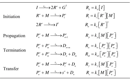
Methyl methacrylate normally is produced by a free radical, chain addition polymerization. Free radical po-lymerization consists of three main reactions: initiation, propagation and termination. Free radicals are formed by the decomposition of initiators. Once formed, these radi-cals propagate by reacting with surrounding monomers to produce long polymer chains; the active site being shifted to the end of the chain when a new monomer is added. During the propagation, millions of monomers are added to 1 radicals. During termination, due to reac-tions among free radicals, the concentration of radicals decreases. Termination is by combination or dispropor-tionation reactions. With chain transfer reactions to monomer, initiator, solvent, or even polymer, the active free radicals are converted to dead polymer [1]. Table 1
o
[image:2.595.310.537.91.229.2]P
Table 1. Polymerization mechanism.
1
2
2 2
d
i
ti o k
d d
o k o o
i i
o k o
ti ti
I R G R k I
R M P R k R M
R I R k R
Initiation
1
d
o k o
n n p p
o n P MP R k M P
Propagation
tc
tc
o o k o o
n m n m tc tc n m
o o k o o
n m n m td td n m
P P D R k P P
P P D D R k P P
Termination
1
f
s k
o o
n n f f
o k o
n n s s
P M P D R k M P
P M s D R k M P
o
n o n
Transfer
gives the basic free radical polymerization mechanism. The free radical polymerization rate decreases due to reduction of monomer and initiator concentration. How-ever, due to viscosity increase beyond a certain conver-sion there is a sudden increase in the polymerization rate. This effect is called Trommsdorff, gel, or auto-accelera-tion effect. For bulk polymerizaauto-accelera-tion of methyl methacry-late beyond the conversion, reaction rate and mo-lecular weight suddenly increase. In high conversion, because of viscosity increase there is a reduction in ter-mination reaction rate.
20%
[image:2.595.311.538.534.720.2]3. Mathematical Modeling of Polymerization
Table 2 shows the mass and energy balances of reactor.
The polymer production is accomplished by a reduction in volume of the mixture. The volumetric reduction fac-tor is given by:
p m p
(1)
The instantaneous volume of mixture is given by:
Table 2. Mass and energy balances.
00 0
d 2
1 d
d
p f
x fk
I k k x
t M V
d d
d d d
I I V
k I
t V t
0
d d
d s d
S S V
k S
t V t
0
d d
d m d
V M x
x
t t
d dt
0
d d
p p p r j
T
mC H k M V UA T T UA T T
t
d d
o j
o p r j o j
T
m C P P UA T T UA T T
t
0
2 d
t
fk I k
M. ABBASZADEH 228
0 1 m MV x
(2)
1 exp 1 p p D A B (5) The parameter is defined as:Similarly, termination rate constant, kt, is given by:
1 s s f f
(3)
0
0
1 1
t t t
k k D
(6) During the free radical polymerization, the cage, glass,
and gel effects occur. For the cage effect, the initiator efficiency factor is used. The CCS (Chiu, Carrat, and Soong) model is used in this study to take into considera-tion the glass and the gel effects. Therefore, propagaconsidera-tion rate constant, kp, is changing according to:
0
t is changing as Arrhenius function.
k p and t
are adjustable parameters related to propagation and ter-mination rate constants, respectively. All the other nec-essary parameters and constants for this model are given in the literature [1]. The Equations (7)-(10) are essential for dynamic studies.
0
0
1 1
p p p
k k D
(4)
1 2 d 1 d , , d p f t fk I xk k x
t k
f x I T
(7)
0
p
k is changing as Arrhenius function, and is
given by equation:
D
2 d 2 1 d 1 dd p f
t
I f
k I k k I x f x I T
t x k
, ,
k I (8)
0 0 3 2 1 d , , , d dp p r j
t
j p
fk I
H k V M x UA T T UA T T
k T
f x I T T
t mC
(9)
4 2 d , , d o j jj r o
j o p
P UA T T UA T T
T
f T T P
t m C
(10)
Equations (7) and (8) are mass balances for monomer and initiator, respectively. Long Chain Approximation (LCA) and Quasi Steady State Approximation (QSSA) are used in this study. Equations (9) and (10) show en-ergy balances for the reactant mixture and oil,
respec-tively. In this study, heat transfer coefficients are esti-mated experimentally [2]. Equations (7)-(10) are highly nonlinear and, using Taylor expansion series, these equa-tions were converted to linearized form. The linearized state space form is given by:
1 1 1
2 2 21
3 3
0 d
d 0
d 0 0
d 0
d
2 d
d
d 0 0
s s
s
s s s
r r
j
s s p p
o po j
r o
r
o po o po
f f f
X x I T
t
X
f f f
i
x I T i
t
T
T f f UA UA UA
t x I mC mC T
m C T
UA UA
UA t
m C m C
0 0 1 0
where
, ,
,
s s
j j js s
,
s
X x x i I I T T T
T T T P P P
(12)
Equation (11) and is converted to the transfer function form:
2
3 4 5 4 3 2 1 2 3 4
( ) ( )
n s n s n T s
P s d s d s d s d s d
5 (13)
4. The Experimental Setup
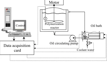
A schematic representation of the experimental batch reactor setup is shown in Figure 1. The reactor is a
Bu-chi type jacketed, cylindrical glass vessel. A multi-pad-dle agitator mixes the content. A Pentium II 500 MHz computer is connected to the reactor via an ADCPWM- 01 analog/digital Input/Output data acquisition card. The data acquisition software was developed in-house. The heating oil was circulated by a gear pump and its flow rate was about 15lit min. The heating/cooling system of the oil consisted of two 1500W electrical heaters and a coolant water coil, which was operated by an On/Off Acco brand solenoid valve. Two Resistance Temperature
Detectors (RTDs), were used with accuracy of .
Methyl methacrylate and toluene were used as monomer and solvent, respectively. Benzoyl peroxide (BPO) was used as the initiator. The molecular weight of the pro-duced polymer was measured using an Ubbelohde vis-cometer.
o
0.2 C
5. An Overview of MPC
Due to its high performance, Model predictive control method has recieved a great deal of attention to control chemical processes, in last few years. This approach is applicable to multivariable systems and canstrained sys-tems. Monuverability in design, noise and disturbance rejection and robustness under model mismatch are the most important ability of this method. Cumbersome
Motor
Data acquisition card
T T
Polymerization
reactor Oil bath
Coolant water
Oil circulating pump
[image:4.595.63.280.581.710.2]Control
Figure 1. The experimental setup.
computation, lack of systematic rules for controller tun-ing are some drawback of this method. Model predictive control is based on a process model. Although impulse or step responses have some limitation for nonlinear proc-ess, they may be used to develop a model. During the the model predictive control following steps should be con-ducted:
Explicit prediction of future output (prediction hori-zon).
Calculation of a control sequence based on the mini-mized cost function (control horizon).
Receding strategy.
The Dynamic Matrix Control (DMC) is used in this research. Its cost function is:
1 1
2 2
1 1
1
N P M
Q R
i N i
J e t i u t i
(14)where P, M and N1 are prediction horizon, control
hori-zon and pure time delay, respectively, RM M , QPP are
whigthing martices. The prediction horizon must be at least equal to the pure time delay.
d p
d m
e t i y t i y t i
y t i y t i d t i
(15)
where ypis the process output, ymis the model output and
d is the process and model outputs diffrence, including noise, disturbance and model mismatch. yd(t) is the
de-sired output based on the refrence input. If ysp(t) is the
refrence input, the following filtered form is used as the tracking trajectory:
1
1
( ); 0d d sp
y t y t y t 1 (16)
changes the first order smoothing filter pole place. The smaller the faster output. It has been shown that system robustness can be decreased by the reduction of
and increment of the manipulated signal [12]. Figure 2 shows the block diagram of DMC.
The cost function in equation 10 can be rearrenged to:
T
Tm D m D
J Y D Y Q Y D Y U R U (17)
without loss of generality, if N1 is assumed zero, then:
Model ym -ysp
M , P
System
d R , Q α
yp
+ u(i-1)
Δu(i-1)
[image:4.595.308.540.611.703.2]Optimization + u(i)
M. ABBASZADEH 230
For LTI system, without any constraints on output or co
where:
1
TYmym t ym tP
1
TD d d
Y y t y tP
1 ,
1
T T
U u t u t M
D d t d t P
ntrol signal, optimization has the following closed form:
T
1 TU G QG R G QE (18)
P D E Y Y
(19)
s are the step response samples and G+ is a Toeplitz
m
N
(20)
where N is the number of system step response samples
1
1
,
1
P
T
g
g g
G
g
U U u t u t M
i
g
atrix consisting the step response samples. The model output has calculated by:
Y G U G
1 2 1
2 1
,
u t 1 u t 1
m N
N
N
p
T
U g U
g g g
g g
G
g
U N
reaching to steady state or equvalent impulse response steps which lead to zero; and gN is the system dc gain.
N
g dcgain
1
1
TN
U u tN u t N u t N P
6. The Modified DMC
If there is any pole close to origin, the step response will
-co
be very slow and the required N is very large. Then, a system including integrator never reaches to the steady state (this case exists in the set of linearized models of the MMA reactor) and N lead to infinity. Hence, unsta-bility occurs. This is one of the DMC limitations [13].
Researchers have suggested some methods to over me this problem, for example formulating DMC in the state space an then using an state observer [14]. Because
of model mismatch this method doesn’t have proper per-formance in real time applications. The alternative is:
m N N
Past N N m Past
Y G U g U Y G U Y
Y GU GU g U
(21)
where YPast
utp
is “the effect of past input to the future system o uts without considering the effect of present and future inputs”. Consequently, YPast can be
calcu-lated by setting the future “Δu”s equ zero and
solv-ing the model P steps ahead.
U Y
al to
m YPas
t (22)
As seen in equations 14 and 15, G+ and U are
inde-pendent of N. Gdimension is determined by N.
There-fore, the DMC culation is independent than N. YD is:
1
Tcal
D d d
Y y t y tp (23)
[image:5.595.63.291.201.345.2] [image:5.595.310.534.515.707.2]7. Results and Discussion
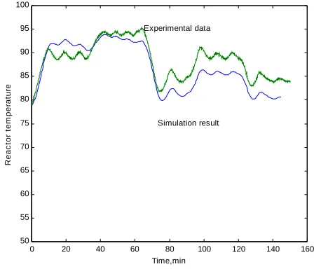
Figure 3 shows the model validation results. The
simu-lation follows the experimental data very well. The DMC algorithm was applied to control a MMA polymerization reactor. The reactor temperature trajectory is known, hence, the refrence input is known for all times so the programmed MPC is used. The DMC controller gain defined as:
T
1 TDMC
K G QG R G Q (24)
DMC
U k E
The
(25)
G ch
of present model is use DMC
kD
d to calculate its k . MC is anged in the appropriate model switching
in-stant. Therefore, a multiple model strategy is used im-plicitly. However the valid model is known before.
0 20 40 60 80 100 120 140 160
50 55 60 65 70 75 80 85 90 95 100
Time,min
Rea
c
tor
t
em
p
er
at
u
re
Experimental data
Simulation result
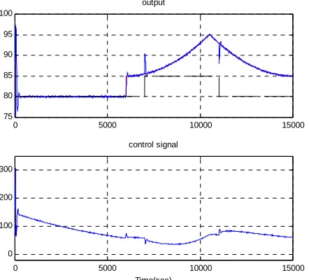
Figures 4 an ity to track the
te
d 5 show the controller abil
mperature trajectory. The average error is 0.3˚C. Due to the controller robustness, switching between models causes no unstability in closed loop system. Furthermore, appropriate selection of controller parameters could pre-vent the unstability. The selected sampling period is T =
10s. Other parameters are P5, M 2, 0.05,
5*5
QI , R.05*I3*3. The ti ip l
nsures the reactor temperature tracking error to with in 0.3˚C while the adaptive PI con-trol in [11] has a 2˚C average error and the Generalized Takagi-Sugeno-Kang fuzzy controller proposed in [16] has a 1˚C average error; demonstrating the superior per-formance of the MPC.
adap ve mult le mode MPC designed here e
0 5000 10000 15000
75 80 85 90 95 100
output
0 5000 10000 15000
0 500 1000 1500
control signal
[image:6.595.64.285.490.690.2]Time(sec)
Figure 4. Controller performance in the absence of distur-bance and noise.
0 5000 10000 15000
75 80 85 90 95 100
output
0 5000 10000 15000
0 100 200 300
control signal
Time(sec)
Figure 5. Controller performance in the presense of ste
zed model based predictive controller based on the DMC algorithm was designed to control the
. C. Carratt and D. S. Soong, “Modeling the Free Radical Solution and Bulk Polymerization of
p disturbance (dashed line) and Guassian measurement noise.
8. Conclusions
A sequential lineari
temperature of a batch MMA polymerization reactor. Using the mechanistic model of the polymerization, a transfer function was derived to relate the reactor tem-perature to the power of the heaters. The coefficients of the transfer function were calculated along the selected temperature trajectory by sequential linearization. The controller performance was studied experimentally on a small scale batch reactor.
9. References
[1] B. M. Louie, G
Methyl Methacrylate,” Journal of Applied Polymer Sci-ence, Vol. 30, No. 10, 1985, pp. 3985- 4012.
doi:10.1002/app.1985.070301004
[2] M. Rafizadeh, “Non-Isothermal Modeling o Polymerization of Methyl Methacr
f Solution ylate for Control
Pur-dern Polymerization Pilot-Plant for
Under-ibatch
Polymeri-coll, “Polymer Reaction Engineering: Modeling poses,” Iranian Polymer Journal, Vol. 10, No. 4, 2001, pp. 251-263.
[3] S. A. Mendoza-Bustos, A. Penlidis and W. R. Cluett, “Use of a Mo
graduate Control Projects,” Chemical Engineering Edu-cation, Vol. 25, No. 1, 1990, pp. 34-39.
[4] T. Peterson, E. Hernandez, Y. Arkun and F. J. Schork, “Non-linear Predictive Control of a Sem
zation Reactor by an Extended DMC,” American Control Conference, Pennsylvania, 21-23 June 1989, pp. 1534- 1539.
[5] A. Penlidis, S. R. Ponnuswamy, C. Kiparissides and K. F. O’Dris
Consideration for Control Studies,” The Chemical Engi-neering Journal, Vol. 50, No. 2, 1992, pp. 95-107. doi:10.1016/0300-9467(92)80013-Z
[6] M. Soroush and C. Kravaris, “Non-linear Contro Batch Polymerization Reactor: An Experimental Study,” l of a AIChE Journal, Vol. 38, No. 9, 1991, pp. 1429-1448. doi:10.1002/aic.690380914
[7] S. De, B. J. Mauricio, J. C. Pinto and E. L. Lima, “C trol of a Chaotic Polymerization Reactor: A Neural Net- on-work Based Model Predictive Approach,” Polymer En-gineering & Science, Vol. 36, No. 4, 1996, pp. 448-457. doi:10.1002/pen.10431
[8] T. Clarke-Pringle and J. F. MacGregor, “Non-linea Adaptive Temperature C
r ontrol of Multi-Product, Semi- Batch Polymerization Reactors,” Computers & Chemical Engineering, Vol. 21, No. 12, 1997, pp. 1395-1409. doi:10.1016/S0098-1354(97)00013-6
[9] R. K. Mutha and W. R. Cluett and A. Penlidis, “On-L Non-linear Model-Based Estimation
ine and Control of a Polymer Reactor,” AIChE Journal, Vol. 43, No. 11, 1997, pp. 3042-3058. doi:10.1002/aic.690431116
Adap-M. ABBASZADEH 232
Science, Vol. tive Model-Predictive Control to a Batch MMA Polym-erization Reactor,” Chemical Engineering
53, No.21, 1998, pp. 3728-3739. doi:10.1002/aic.690431116
[11] M. Rafizadeh, “Sequential Linearization Adaptive Con-trol of Solution Polymerization of
a Batch Reactor,” Polymer R
Methyl Methacrylate in eaction Engineering, Vol. 3, No. 10, 2002, pp. 121-133.
doi:10.1081/PRE-120014692
[12] R. Rouhani and R. K. Mehra, “Model Algorithmic Con-trol; Basic Teoretical Properties,” Automatica, Vol 18, No 4, 1982, pp. 401-404.
doi:10.1016/0005-1098(82)90069-3
[13] E. F. Camacho and C. Bordons, “Model Predictive Con-trol in the Process Industry,” Springer and Verlag, New
Dynamic Matrix Control,” Computers
ntrol of Open Loop Unstable Processes,”
Pro-olymerization Reactor York, 1995.
[14] P. Lundstorm, J. H. Lee, M. Morari and S. Skogestod, “Limitations of
& Chemical Engineering, Vol. 19, No. 4, 1995, pp 402- 421.
[15] Q. Z. Kent, D. G. Fisher and A. Alberta, “Model Predic-tive Co
ceedings of the American Control Conference, San Frav- cisco, 10 June 1993, pp. 791-795.
[16] R. Solgi, R. Vosough, and M. Rafizadeh, “Adaptive Fuzzy Control of MMA Batch P