Versatile Gaussian probes for squeezing estimation

Versatile Gaussian probes for squeezing estimation

Luca Rigovacca,1Alessandro Farace,2Leonardo A. M. Souza,3,4Antonella De Pasquale,5 Vittorio Giovannetti,5_{and Gerardo Adesso}4

1_{Blackett Laboratory, Imperial College London, London SW7 2AZ, United Kingdom} 2_{Max-Planck-Institut fur Quantenoptik, Hans-Kopfermann-Strasse 1, 85748 Garching, Germany} 3_{Universidade Federal de Viçosa - Campus Florestal, LMG818 Km6, Minas Gerais, Florestal 35690-000, Brazil}

4_{Centre for the Mathematics and Theoretical Physics of Quantum Non-Equilibrium Systems (CQNE), School of Mathematical Sciences,} University of Nottingham, University Park, Nottingham NG7 2RD, United Kingdom

5_{NEST, Scuola Normale Superiore and Istituto Nanoscienze-CNR, I-56126 Pisa, Italy} (Received 16 March 2017; published 16 May 2017)

We consider an instance of “black-box” quantum metrology in the Gaussian framework, where we aim to estimate the amount of squeezing applied on an input probe, without previous knowledge on the phase of the applied squeezing. By taking the quantum Fisher information (QFI) as the figure of merit, we evaluate its average and variance with respect to this phase in order to identify probe states that yield good precision for many different squeezing directions. We first consider the case of single-mode Gaussian probes with the same energy, and find that pure squeezed states maximize the average quantum Fisher information (AvQFI) at the cost of a performance that oscillates strongly as the squeezing direction is changed. Although the variance can be brought to zero by correlating the probing system with a reference mode, the maximum AvQFI cannot be increased in the same way. A different scenario opens if one takes into account the effects of photon losses: coherent states represent the optimal single-mode choice when losses exceed a certain threshold and, moreover, correlated probes can now yield larger AvQFI values than all single-mode states, on top of having zero variance.

DOI:10.1103/PhysRevA.95.052331

I. INTRODUCTION

Quantum metrology is one of the most developed fields within the framework of quantum information, and it has been the object of several studies in the last decade [1–7]. As a matter of fact, precise measurements and observations are a fundamental part of the scientific method and the possibility of exploiting quantum mechanics in order to improve the estimation precision over the best classical strategy is thus very appealing. Quantum metrology finds application in a wide range of situations where one is interested in gaining precise information about a system or a physical process [8–12].

In order to gather information about a certain system, the most common approach consists of sending a known probing system to it, collect the probe after it had the chance to interact with the target system, and look for differences with respect to the original state that was sent in. From this comparison, our knowledge about the state of the target system and/or the physical processes taking place during the interaction can be improved. In analogy with this simple schematic picture, a typical estimation protocol can be divided into three steps: (i) probe preparation, (ii) interaction between probe and system of interest, and (iii) readout measurement on the evolved state of the probe. These three stages are not independent from each other, and the quality of the overall estimation depends on how well they work together. For example, when the probe is being prepared one should make sure it can be significantly altered by the process under investigation. Similarly, any change in the probe is not useful at all if it cannot be detected by the performed measurement. Here, as in most theoretical studies, we focus on the interplay between the first and the second stage mentioned above. We assume that any measurement allowed by the laws of quantum mechanics can be performed, and we investigate how to tailor the choice of the probe depending on the information available at the first stage.

to a good estimation precision over the whole set of possible interactions, and which are the resources responsible for this behavior.

A scenario of black-box metrology has been recently studied for unitary encodings in finite-dimensional systems, where the eigenvalues of the generating Hamiltonian are fixed and known, while the exact eigenbasis is left unspecified [13,15–17]. One way to ask for versatility is to maximize the worst-case estimation precision over the set of possi-ble encodings (or equivalently over the set of isospectral Hamiltonians). In this case it has been found that the input probe needs to be correlated with another ancillary system, which is kept as a reference and measured together with the probe at the measurement stage. This is because any local probe undergoing a unitary evolution is left unchanged by a Hamiltonian diagonal in its same eigenbasis and the worst-case precision becomes trivially zero. Although entangled states guarantee the highest minimal precision, interestingly the presence of entanglement is not a necessary condition in order to obtain a nonzero worst-case performance [18–21]. Indeed, the key resource in this and similar discrimination tasks is a weaker form of correlation known as “quantum discord” [22,23]. A complementary approach to versatility consists of looking for the probe that guarantees the bestaverage(instead of minimal) performance. In Ref. [24] it is shown that from this perspective the presence of correlations is helpful but does not represent the only important parameter, as local purity also plays a fundamental role.

When continuous variable systems are concerned, one typically considers additional realistic constraints on the probe (such as finite energy, finite correlations) which give access only to a limited portion of the Hilbert space and make the analysis more involved. Up to now only the former of the two aforementioned approaches to black-box metrology (i.e., guaranteeing minimal performances) has been investigated in the framework of Gaussian states and operations [25–27], and quantum discord has once again been identified as the impor-tant figure of merit for these discrimination tasks [28–30].

In this work, we move forward along two different directions. On one hand, we take the perspective of looking at the average performance associated with a certain input Gaussian probe. On the other hand, in the second half of this paper we also study the effects of a noisy encoding operation, moving away from the most common unitary setting. It is worth stressing that in all previous studies of Gaussian black-box metrology, the set of possible encoding Hamiltonians has been obtained by applying a generic Gaussian unitary operation to a harmonic Hamiltonian [28–30]. Although this choice represents the Gaussian equivalent of a generic change of basis in the finite-dimensional domain, it has the disadvantage of introducing energy into the probe, at random and for free. This is because a generic Gaussian unitary operation includes the application of squeezing. Intuitively, adding energy to the probe increases the estimation precision. While this does not affect the study of the worst-case precision, it can instead arbitrarily increase the average precision. Therefore, to make our model meaningful, we will apply only “passive” Gaussian unitary operations (e.g., optically obtainable via beamsplitters and phase shifters) to a fixed seed Hamiltonian. In the following we will choose the seed Hamiltonian to be

a single-mode squeezing Hamiltonian, and passive Gaussian unitaries are then identified by all single-mode phase rotations. The problem of estimating the parameter of a squeezing Hamiltonian has been investigated in the past, by looking at its effect on the Hilbert space of the radiation field [31,32], or by using Gaussian [33–35] or non-Gaussian probes obtained via Kerr interactions [36]. The goal of this paper, instead, is to understand which Gaussian probe yields the optimal average performance for the task of estimating the amount of squeezing applied on the probing system by an external device, without prior information on the direction of application. This direction could be fixed, but initially unknown, or could randomly fluctuate from one encoding operation to another. If the state of the probe that will be used in all experiments is fixed beforehand, our results indifferently apply to both these scenarios, as long as full information on the direction is available at the measurement stage. In particular, we want to discuss whether the presence of input correlations can lead to an improvement over the optimal single-mode result. We start by considering a noiseless setup, and we characterize the single-mode states that yield the best average estimation precisions. We compare their performance with the precision obtainable by sending half of a two-mode squeezed state to the squeezing device, while keeping the other half as reference. Although the average estimation precision reached by this paradigmatic class of correlated bipartite states equals that of the optimal single-mode probes, we can show that the correlated probes have the advantage of a stable performance over all squeezing direction, at the cost of introducing extra photons for the reference beam. The advantage of using correlations will become even more important when noise is added to the process, in the form of photon losses during the transmission of the probe signal to and from the squeezing device. Indeed, a numerical analysis reveals how in this case the presence of correlations can even improve the average precision over the value associated with the optimal single-mode probe.

The following sections are organized as follows. After presenting some preliminary notions in Sec. II, in Sec. III we formally introduce the black-box metrology model we are considering, and show a physical situation where it could arise. We analytically solve the problem in absence of noise in Sec.III A, while in Sec.III Bwe numerically study the same situation in presence of losses. We present our conclusions in Sec.IV, and further technical comments can be found in the appendices.

II. PRELIMINARY NOTIONS

A. Estimation theory and quantum Fisher information The problem of estimating a parameter characterizing a certain evolution by repeatedly measuring its output has a long history and was originally studied in a classical framework. The typical situation here involves a parameter-dependent probability distributionp(x|). The goal is to obtain the best possible estimation of the parameter by sampling many times the random variablex distributed according top(x|). A well known result in classical estimation theory, which goes under the name of the Cramér-Rao bound [39], states that the root-mean-square error (RMSE) of any unbiased estimator ˆ of the parameterhas to satisfy the following inequality:

δˆ √1

MF. (1)

On the right-hand side,Mrepresents the number of performed samplings, andF is the Fisher information of the process, defined by

F=

dx p(x|)[∂lnp(x|)]2. (2)

Importantly, the bound in Eq. (1) can be saturated in the asymptotic limit of many measurements, for example if the estimator ˆ is obtained by maximizing the likelihood of the recorded events.

In the quantum counterparts of the aforementioned situ-ation, the parameter is encoded in a quantum state ρ, typically obtained by applying a completely positive and trace-preserving (CPT) map to a known input probe ρ [40], so that

ρ=[ρ]. (3)

In order to obtain information about the encoding device, and thus on , a generic positive-operator-valued measurement (POVM) has to be performed onρ. This kind of measurement is characterized by a set of positive operators{Ex}x, satisfying

xEx =1. Once applied on the encoded states, it yields the measured valuexwith probability

p|_{Ex}x(x|)=Tr [ρEx], (4)

from which the associated classical Fisher informationF|_{Ex}x can be evaluated via Eq. (2). Clearly, the ultimate precision allowed by quantum mechanics for the unbiased estimation of is obtained by optimizing over all POVMs. In this way, it is possible to obtain the quantum Cramér-Rao bound [37], which states

δˆ √ 1

MH(ρ), (5)

whereHis the quantum Fisher information (QFI) associated with the encoded stateρ, obtained fromρas in Eq. (3). This quantity is defined as

H[ρ]=TrρL2

, (6)

whereLis a Hermitian operator which goes under the name of symmetric logarithmic derivative (SLD) and satisfies the relation

ρL+Lρ=2∂ρ. (7)

Alternatively, it has been shown that the QFI is closely related to the second-order expansion of the Bures distance [41], or equivalently of the Uhlmann fidelity F(ρ1,ρ2)=

(Tr [√ρ1ρ2√ρ1]) 2

[42]:

H[ρ]=8 lim d→0

1−√F(ρ,ρ+d)

d2 . (8)

Rigorously speaking, this last equality is true as long as the rank ofρdoes not change in correspondence of the value of in which Eq. (8) is calculated. If this should not be the case, Ref. [43] recently showed that Eq. (8) should be corrected by adding a term that involves second derivatives of the vanishing eigenvalues. As a consequence, the QFI might become discontinuous at those pathological points. Finally, if one is interested in obtaining the ultimate precision for the estimation of the parameter characterizing the CPT encoding map, an optimization has to be performed over the probeρ.

We conclude this overview of quantum estimation theory with a few remarks. At first, let us point out that the projective measurement on the eigenbasis of the SLD operator L has always a Fisher information equal to the QFI [37]. This assures that the bound of Eq. (5) is a priori tight, even though the necessary control needed to perform this particular measurement is often out of experimental reach. Even in this situation, however, the QFI can be considered a figure of merit for the probe state, which has the potential to be very susceptible to small changes of the parameter that characterizes the encoding channel. As a second remark, note that in general the QFI depends on the real parameter. This is why the QFI gives the ultimate precision attainable in a localestimation: typically one already has some knowledge of , and is interested in finding small fluctuation around this approximately known value. The situation simplifies for unitary encodings, wherecan be actually written asUρU†, withUU†=U†U=1andrepresents a global phase [44]. In this case,H(ρ) is independent from, and therefore so is the ultimate precision attainable byρ.

B. Gaussian states of continuous variable systems In this paper we consider continuous variable systems composed by one or two bosonic modes described by the annihilation operators ˆa and ˆb, which satisfy the canonical commutation relations

[ ˆa,ˆa]=[ ˆb,b]ˆ =[ ˆa,b]ˆ =[ ˆa,bˆ†]=0, (9)

[ ˆa,aˆ†]=[ ˆb,bˆ†]=1. (10)

In the following we will label withAandBthe systems associ-ated with the modes described respectively by ˆaand ˆb. The as-sociated quadratures ˆxA=( ˆa†+a)/ˆ √2,pAˆ =i( ˆa†−a)/ˆ √2, and similarly ˆxB and ˆpB, can be combined to form the vector ˆr=( ˆxA,pA,ˆ xB,ˆ pBˆ ). This appears in the definition of the covariance matrix associated with any state ρ of this continuous variable system:

where {·,·}₊ represents the anticommutator andξξξ =Tr [ρˆr] is the associated displacement vector. The Robertson-Schrödinger uncertainty relation, which all physical states must satisfy, in this language can be written as

+i 000, (12)

where is the standard symplectic form

=

j

0 1

−1 0 . (13)

Here, and whenever not explicitly mentioned, the sum overj runs over the two bosonic modes of the system.

In this paper we will focus on Gaussian states, defined as those density matricesρ characterized by a characteristic functionχρ(z)=Tr [ρ e−iz ˆr_{], withz∈R}2_{, that is the inverse}

Fourier transform of a Gaussian function. They are completely characterized by the first and second moments of the latter, i.e., by the vectorξξξ and the matrixpreviously defined. At this point it is useful to mention Williamson’s theorem, which allows us to decompose every covariance matrix into the form

=T DT. (14)

Here, T is a matrix of the real symplectic group Sp, i.e., such thatT T= , andD=_jνj12 is a block-diagonal

matrix whose blocks are multiples of the 2×2 identity matrix. These proportionality coefficients{νj}jare called “symplectic eigenvalues” of the Gaussian states, are constrained by Eq. (12) to be larger than or equal to 1, and can be found as regular eigenvalues of the positive-definite matrix |i |. A pure Gaussian state is characterized by νj ≡1, and we refer to a state withT =1as to a “thermal state.”

A unitary evolutionU that maps the set of Gaussian states into itself can be fully characterized by its action onˆr:

U[ˆr]=U−1ˆr+ξξξ(U), (15) whereU ∈Spandξξξ(U)is a real vector. The particular Gaussian unitary evolutions that will be considered in this work are characterized byξξξ(U)=000. In this case, the covariance matrix and the displacement vector associated with U[ρ] can be written in terms of ξξξ and , which characterize the input Gaussian stateρ, via the following mapping:

−→U U U, ξξξ−→U Uξξξ . (16)

In particular, we will focus on single-mode phase rotations and squeezing operations, that take an input state ρA re-spectively to R(θA)[ρA]=e−

iθaˆ†aˆ_ρAe+iθaˆ†aˆ

and Sα(A)[ρA]= e−α2( ˆa†2−aˆ2)ρAe+

α

2( ˆa†2−aˆ2). These Gaussian unitary maps can be

characterized by the symplectic matrices:

R_θ(A)=

cosθ sinθ −sinθ cosθ , S

(A)

α =

eα ₀

0 e−α , (17)

which take the role ofUin Eqs. (15) and (16). The first of these operations simply rotates the quadratures of the state in phase space, while the effect of squeezing is to reduce the variance of one quadrature while increasing the other. The CPT maps that preserve the Gaussian character of a state are not limited to the set of Gaussian unitary evolutions, but include also

several noisy operations [45]. In particular, in the following we will consider the lossy channelLη, parametrized byη∈[0,1]. When applied on the first mode of a two-mode state, it modifies the input covariance matrix and displacement vectorξξξ as follows:

L

(A)

η

−→KηKη+NηNη, ξξξ L(A)

η

−→Kηξξξ , (18)

whereKηandNηare the block-diagonal matrices

Kη =

_√

η12

12

, Nη=

√

1−η12 _{, (19)}

with empty blocks being composed only by zeros.

Due to their simplicity and practical relevance, Gaussian states form the most studied class of density matrices in continuous variable systems. In particular, many quantum information quantifiers can be written in closed form when evaluated on Gaussian states. In the following we will focus on the QFI, which thanks to Eq. (8) has been explicitly evaluated for single-mode [38], two-mode [34], and for generic multimode Gaussian states [46]. These formulas, or a perturbative approach based on Eq. (8), have been recently employed in order to assess the performance of Gaussian states in various estimation tasks [35,47]. We report here the expression for the QFI of a two-mode probeρAB[34]:

H[ρAB]= 1

2(|M˜| −1){| ˜

M|Tr [( ˜M−1M)˙˜ 2]

+

|1+M˜2_{|Tr [((1+}M˜2)−1M)˙˜ 2]}

+ 4

2(|M˜| −1)

˜

ν₁2−ν˜2₂− ν˙˜

2 1

˜ ν₁4−1 +

˙˜ ν2₂ ˜ ν₂4−1

+2 ˙˜ξξξ˜−1ξξξ ,˙˜ (20)

where the symbol | · | represents the determinant, the dot corresponds to the derivative with respect to, and we defined M=i . The tilde appearing on top of all quantities reminds us that they have to be evaluated on the encoded state[ρAB]. This formula has a first contribution which depends on the whole covariance matrix, a second one which explicitly takes into account the variation of the symplectic eigenvalues, and a third one which accounts for changes in the displacement vector of the encoded state. In particular, we point out that the second contribution can lead to irregular behaviors when the encoded stateρhas at least one eigenvalue equal to 1 [34,43]. In what follows we can safely ignore this problem because we will consider either (i) unitary encodings, which do not change the symplectic eigenvalues, or (ii) mixed encoded states with no symplectic eigenvalue equal to 1.

In the last part of this section, we explicitly consider a local encoding =(A)⊗1B acting nontrivially only on subsystem A, and simplify Eq. (20) to obtain the QFI of a single-mode Gaussian state ρA. We will get an expression which is equivalent, but not identical, to the one found in Ref. [38]. This alternative expression will be of great help in the following analysis. Let us start by considering a single-mode channel (A)

of the formρA⊗ρth(νB), whereρth(νB) is a thermal state, characterized byT =12 andD=νB12 in Eq. (14). Thanks

to the factorized structure of probe and channel, no change in precision can possibly arise from choosing a different value forνB. However, the obtained expression forH[ρA⊗ρth(νB)] still depends onνB in a nontrivial way. This dependence is a consequence of the mathematical structure of Eq. (20), but we know that physically the parameterνB cannot play a role in the QFI. Therefore, we can use the trick of considering a factorized probe ρA⊗ρth(νB) in order to easily deduce a relation between M˜A and its derivative, where M˜A is evaluated on the encoded single-mode state(A)

(ρA). After a straightforward manipulation, we can see that the studied QFI is independent fromνB if and only if the following relation holds:

1 |MA˜ |

d|M˜A| d

2

= |_MA˜ _|TrM˜−1

A MA˙˜

2

−(1− |MA˜ |)2Tr1+M˜_A2−1MA˙˜ 2. (21)

This can now be used to substitute either Tr[( ˜M_A−1MA)˙˜ 2] or (d|M˜A|

d )

2 _{in the remainder of Eq. (20), in order to obtain an}

expression for the QFI of a single-mode probe, labeled by H(1)

. With the former choice, this becomes

H(1)(ρA)= |MA˜ | −1

2 Tr

1+M˜_A2−1M˙˜A

2

+ 1

2(|M˜A|2−1)

d|M˜A|

d

2

+2 ˙˜ξξξ_A˜_A−1ξξξ˙˜A, (22)

where ˜Aand ˜ξξξAare respectively the covariance matrix and the displacement vector associated with(A)(ρA). With respect to the expression of Ref. [38], this is advantageous in all those situations where Tr{[(1+M˜2

A)−1MA]˙˜ 2}is easier to compute than Tr [( ˜M_A−1M˙˜A)2_{], as in Sec.III Bbelow.}

III. VERSATILE GAUSSIAN PROBES FOR SQUEEZING ESTIMATION

As mentioned in the introduction, we want to study a problem of black-box metrology in which the parameter to estimate is the strength of the squeezing applied on the probing state, and an additional uncertainty affects the direction θ in which the squeezing operation is applied. In absence of noise, the overall encoding CPT map acting on modeAcan thus be written as

_,θ(A)≡S(A)◦R(_θA), (23)

where ◦ represents the usual composition of maps. In our analysis we are going to assume that the angleθ is picked randomly from [0,2π] and is unknown at the stage in which the probes are being prepared. Yet we shall assume that the selected value ofθis revealed after the parameterhas been imprinted into the system. Accordingly, while the presence ofθ cannot be trivially compensated by properly antirotating the input states of the probes, the knowledge of its value can influence the design of the optimal POVM measurement. For

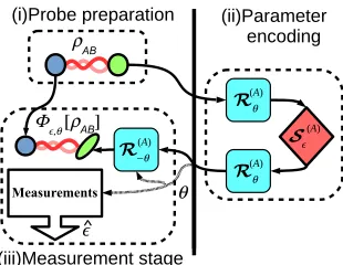
FIG. 1. Sketch of a physical scenario in which a squeezing operation along an initially unknown direction is applied on the probing system. Stage (i): versatile single-mode or two-mode probes are prepared, without knowing the angle θ characterizing the estimation process in which they will be used. Stage (ii): the probing systems are sent to the squeezing device, and in each one-way trip they acquire a certain phaseθ. Stage (iii): upon recollection of the probes, the angleθ becomes known, and can be used to devise the best measurement allowed by quantum mechanics, from which an estimator ˆis recovered. Note that the knowledge ofθ can also be used to apply the unitary correction R(A)_−θ on the final state of the probes. Although this does not change the QFI, it allows us to write the total encoding unitary operation in the same form that appears in Eq. (23).

example, as schematically shown in Fig.1, this scenario can arise in an optical setup if the distance from a squeezing device, which appliesSto the input state, is not known in advance or is fluctuating from one measurement to the other. In its trip to and from the squeezer, the light will be affected by the free evolution R(θA), so that each probe actually evolves via R(A)

θ ◦S(A)◦R

(A)

θ . Althoughθis not known when the probes are being prepared, in this example its value could be inferred by the light travel time, or it could be independently estimated once the setup has been set, and the estimation experiment is about to be performed. However, it is important to keep in mind that this information can only be used to optimize the readout measurement, and not the states of the probes used in the following experimental runs, because we are assuming that the probing systems have been selected and prepared beforehand. Upon receiving the encoded state, it is, e.g., possible to add a unitary correctionR(₋Aθ) toR

(A)

θ ◦S( A)

◦R

(A)

θ , changing the effective evolution of a single-mode probe ρA to match the form of Eq. (23) (further compensations being possible if required by the measurement optimization stage).

Under the above conditions the quantum Cramér-Rao bound (5) predicts that the ultimate estimation accuracy achievable with a probing stateρexhibits an explicit functional dependence uponθ,

δ(θ)ˆ 1 MH(θ)(ρ)

, (24)

of granting, i.e., the quantity

H(ρ)≡

2π

0

dθ 2π H

(θ)

(ρ). (25)

From Eq. (24) and from the convexity of the function 1/√xit follows thatH(ρ) sets a lower bound on the average value of the attainable RMSEs, i.e.,

δˆ≡

2π

0

dθ

2π δ(θ)ˆ 1

MH(ρ)

. (26)

As explicitly discussed in AppendixA, the AvQFI quantity can be used also to bound the accuracy achievable in an alternative setting where, at variance with the case represented in Fig.1, the phaseθfluctuates over different probing stages.

Although the encoding operation given in Eq. (23) acts only on a single mode of the field, we can nonetheless consider the possibility of using a two-mode probe. In this case, one of its modes (say,A) is sent to the squeezing station, while its second mode (B) is kept unaltered in the laboratory as reference. As often happens, the presence of initial correlations between the two subsystems could potentially help in the estimation of, even if modeBis not directly affected by the evolution. In this more general case, the total encoding map can be written as

,θ(ρAB)=( A)

,θ ⊗1

(B)_{[ρAB]. (27)}

In the remainder of this paper we will label byHthe AvQFI associated with a two-mode probe. In all those situations where we are explicitly using a single-mode probing system, we will emphasize this choice by using the symbolH(1) for the AvQFI. It is now worthwhile to briefly discuss the properties of the AvQFI. In particular, it is convex in the input probe because it inherits this property from the QFI. The AvQFI is also invariant under phase rotations onAand generic unitary evolutionsU(B) applied on modeB, i.e.,

H

R(A)

φ ⊗U(

B)_{[ρAB]=H[ρAB]. (28)}

This can be seen in two steps. At first, U(B) commutes with the encoding channel ,θ, and it can be absorbed in the measurement process, thus leaving the QFI unaltered. Then, notice that

,θ◦R(_φA)[ρAB]=Rφ(A)◦,θ+φ[ρAB]. (29)

Once again, the externalR(φA) can be included in the readout process, while the shift inθvanishes because of the average appearing in Eq. (25). Crucially, we can exploit the symmetry of Eq. (28) in order to simplify the structure of the set of probesρABthat we need to explicitly consider in our search for the optimal average performance. As detailed in AppendixB, it is enough to consider states in the standard form ρ(std)

characterized by

(std)=

⎛ ⎜ ⎝

ax axp c 0

axp ap 0 d

c 0 b 0

0 d 0 b

⎞ ⎟

⎠, ξξξ(std)=(ξx,ξp,0,0). (30)

Equation (30) is a good parametrization for two-mode input states, but whenever we deal with single-mode probes it is convenient to use a different approach. The covariance matrix

and displacement vector of a generic single-mode Gaussian stateρAcan be decomposed as

A=νARφS2αRφ, ξξξA= |ξ|

cosψ

sinψ , (31)

whereνAcharacterizes its thermal excitations,αandφ quan-tify respectively the amount and the direction of squeezing, whileψfixes the displacement direction. After the application of the phase rotation R(θA), the parameters φ and ψ of the evolved state R(θA)[ρA] are respectivelyφ=φ+θ and ψ=ψ−θ. As the average over θ in the AvQFI can be equivalently performed overθ+φ, only the sumφ+ψ can influence the average estimation precision obtained with the probe ρA. For this reason, without loss of generality in the following we can setφ=0 in Eq. (31) when parametrizing single-mode probes.

Although here we explicitly discussed the noiseless unitary encoding given in Eq. (27), we point out that the same reasoning that led us to Eqs. (30) and (31) can be applied also in Sec.III B, where we consider a noisy evolution. This is because we only deal with photon losses, whose CPT map Lη, defined in Eq. (18), commutes with phase rotations.

A. Results for noiseless evolution

In order to find the average performance of a two-mode Gaussian probe state for the estimation of the squeezing param-eter, characterizing the noiseless evolution,θ defined in Eq. (27), we first need to evaluate itsθ-dependent QFI through Eq. (20). We stress that due to the unitarity of the evolution, we can ignore the contribution coming from the derivatives of the symplectic eigenvalues. The remaining terms can be explicitly evaluated for input states of the form of Eq. (30) by writing the matrix ˜Min terms of the input covariance matrixas follows:

Tr [( ˜M−1M)˙˜ 2]=2 Tr−1VθVθ+Vθ2

, (32)

Tr [((1+M˜2)−1M)˙˜ 2]= −Tr [(OVθ+OVθ)2], (33)

where Vθ=R_θ(S−1

S)Rθ˙ and O=(1− )−1 . An analytical, quite involved, expression for the AvQFI can be found in AppendixC.

By settingc,d =0 we can obtain a simpler expression that does not depend onb, which can be interpreted as the average performance of a single-mode probe. Overall, its average QFI can be written as

H(1)[ρA]= Tr [A]

2_{+4 detA}

2(1+detA) +

|ξ|2Tr [A]

detA , (34)

whereAis the input covariance matrix and|ξ| = √

ξ2

x +ξp2. We begin by commenting the single-mode result, and then we move to study the effects of input correlations.

1. Single-mode probes

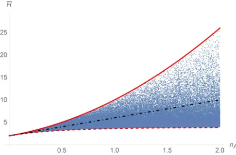
FIG. 2. Noiseless AvQFI for single-mode Gaussian probes with respect to the photon number nA. Blue dots: 105 single-mode Gaussian state uniformly sampled with the method of AppendixE; red top solid line: pure undisplaced squeezed states; red bottom dashed line: undisplaced thermal states; black dot-dashed line: coherent states.

single-mode AvQFI of Eq. (34) can alternatively be obtained by averaging the single-mode QFI for fixed squeezing direction found in Ref. [34]. This can be easily shown by writing their QFI in our notation, for input states parametrized as in Eq. (31) withφ=0:

H_θ(1) = 2|ξ|

2

νA {cosh(2α)+cos[4θ−2ψ] sinh(2α)}

+ 4νA2 ν2

A+1

cosh4α+sinh4α−1

2cos[4θ] sinh

2_{(2α) .}

(35)

Equation (34) can then be retrieved from this expression by averaging overθ.

Since we are dealing with states defined in an infinite-dimensional Hilbert space, we take the physically meaningful approach of looking for the optimal probe under the condition of fixed input energy, i.e., fixed average photon number

nA= νAcosh(2α)−1+ |ξ|

2

2 . (36)

This is because an arbitrary amount of energy can lead to an unbounded estimation precision. A plot ofH(1)(ρA) againstnA for randomly generated single-mode input Gaussian states can be found in Fig.2. We can see that the optimal probe is given by a pure undisplaced squeezed state (|ξ| =0,νA=1), while the worst performance is obtained when an undisplaced thermal state is used (|ξ| =0,α=0). The corresponding AvQFIs are respectively given by

H(1)ρ_A(sq)=4n2A+4nA+2, (37)

H(1)ρ_A(th)=4 (2nA+1)

2

1+(2nA+1)2, (38)

FIG. 3. Range of QFI values that could be achieved for any fixed

nAby varying θ, for pure and undisplaced squeezed single-mode probesρA(sq). The corresponding AvQFI is plotted as a black line for comparison.

while coherent states (α=0,νA=1) have an intermediate scaling

H(1)ρ_A(coh)=2(1+2nA). (39)

Formal proofs of these bounds can be found in AppendixD. For single-mode input probes, we can also study the variance overθof the QFI written in Eq. (35). This is found to be

VAR(Hθ)= V2

1 +V22−2V1V2cos(2ψ)

2 , (40)

where

V1=

2ν2

A ν_A2 +1sinh

2_{(2α), V}

2=

2|ξ|2

νA sinh(2α). (41)

As can be expected, whenξ =0 the variance does not depend onψ. Moreover, it is identically zero when α=0, or when the probe displacement is opportunely chosen so as to have V1 =V2, withψan integer multiple ofπ. Therefore, the QFI of

ρ_A(th)andρ_A(coh)does not depend onθ, as they are characterized byα=0. On the contrary, the variance in Eq. (41) for pure undisplaced squeezed states increases with α, and thus with nA. This implies that the single-mode probes associated with the optimal average performance also yield strong fluctuations in precision with respect toθ. Although the QFI associated with these probes is nonzero for anyθ, an unlucky choice ofθ can bring the estimation precision to its absolute lower bound (QFI=2) (see Fig.3).

2. Two-mode probes

ρA=TrB[ρAB], because the QFI is monotonically decreasing under partial trace. This trivially implies

H[ρAB]H(1)[ρA]min ρA

H(1)[ρA]. (42)

A priori, it might be possible to improve the average estimation precision by exploiting correlations with an ancillary mode, for example by using input entangled states. An obvious candidate in looking for this sort of advantage would be a correlated two-mode extension of the optimal single-mode probe. However, this state does not exists becauseρ_A(sq)is pure and cannot be correlated with any other system. This suggests the presence of a trade-off between pure local squeezing and two-mode correlations, consistently with the results known in the finite-dimensional case [24]. As a paradigmatic example of correlated probes, we study the class of two-mode squeezed vacuum states ρ_AB(sq)(r), usually considered as the continuous variables counterpart of maximally entangled states. In the notation of Eq. (30), their standard parameters areξx =ξp= axp=0 and

ax =ap=b=cosh(2r), c= −d =sinh(2r). (43)

In this case, the general formula for H(ρAB) given in AppendixCgreatly simplifies to

Hρ_AB(sq)=4 sinh(r)4+4 sinh(r)2+2. (44)

Interestingly, for this class of states the number of photon in modeAis equal to sinh(r)2_{and we see that}

Hρ_AB(sq)=H(1)ρ_A(sq)=max ρA

H(1)[ρA]. (45)

Therefore, ρ_AB(sq) yields the same average performances of a pure single-mode squeezed probe. This differs from what has been recently found in a finite-dimensional setting [24], even tough exploiting the average skew information [48,49] as figure of merit, where entanglement was necessary in order to obtain the maximum average precision. We have strong numerical evidences that all other two-mode Gaussian states with the same nA yield worse average precisions thanρ_AB(sq). Another interesting observation is that the QFI associated with ρ_AB(sq) is constant over all choices of θ and equal to its average in Eq. (44). Indeed, due to the symmetry of their covariance matrix [see Eq. (43)], allθ dependencies in Eqs. (32) and (33) cancel. Therefore, even if single-mode and two-mode squeezed states lead to the same average performances with respect to nA, the latter choice removes fluctuations at the cost of doubling the total number of photons N in the probe. Input correlations are therefore beneficial in all those situations where the guarantee of obtaining a certain predictable performance is preferable to the risk of dealing with fluctuations in estimation precision.

Finally, we still have to discuss what happens if we compare the AvQFIs of two-mode and single-mode probes with the same total number of photons N. From Eq. (45) and the numerical evidences in support of the fact that ρ(sq)_AB seems to be the best two-mode probe, it should be clear that with this meter of comparison the presence of a reference beam cannot improve the estimation precision. Indeed, two-mode squeezed

states can match the performance of single-mode squeezed states only at the cost of doubling the total photon number.

B. Results for noisy evolution

Up to now, we considered the ideal and noiseless evolution ,θ defined in Eq. (27). In this section we move to a more realistic scenario by introducing some noise in the picture. In particular, we consider photon losses occurring during the propagation of the probes to and from the squeezing device. The resulting encoding channel acting on subsystemAcan be written as

˜

(_,η,θA) =L(_ηA)◦(_,θA)◦L(_ηA), (46)

where the action of the lossy channel has been detailed in Eq. (18). We consider the loss parameter η to be fixed and known. Differently from before, the physical map that encodes the parameter on the probing system is not unitary. This fact has two main consequences: in general the QFI will be -dependent, and the possible changes in the symplectic eigenvalues of the probe contribute to the QFI via the third line of Eq. (20).

We will show that, in a noisy environment, correlated two-mode probes can lead to higher average precisions than the optimal single-mode input states. It turns out that this is always true when we compare AvQFIs of states with the samenA. Interestingly, the same result can hold even if the comparison is performed by fixing thetotalphoton numberNof the probe state, if the pair (N,η) lies within a certain region.

1. Optimal single-mode probes

In analogy with the noiseless analysis, we are able to find a closed expression for the single-mode QFI in presence of losses. This is one of those cases where our expression for the single-mode QFI, given in Eq. (22), results in being useful. Indeed, when we apply the encoding channel ˜(_,η,θA) to a probe with standard covariance matrix as in Eq. (30), (1+M˜2

A) becomes a multiple of the identity. Its inverse is therefore much easier to compute than the inverse of ˜MA, which would be required if the expression given in Ref. [38] were to be used. The explicit expression for theθ-dependent QFI can be found in AppendixFfor any values ofηand >0. Due to the complexity of the obtained expression, we cannot analytically average it overθin [0,2π], but we can study it numerically.

A first interesting feature is that a dependence on ψ is generally retained even after the average over the squeezing directionθis performed. This is in contrast with the noiseless case, where only the absolute value of the displacement was relevant [see Eq. (34)]. Without loss of generality we can still fixφ=0 in the state parametrization given by Eq. (31). Then, for any fixed values ofnA,,η, andαwe find that the maximum of H,η is reached when ψ= ±π/2. This corresponds to a displacement in the direction of the quadrature with the smallest variance. This fact is formally proven AppendixF.

FIG. 4. AvQFI with respect toνand|ξ|2_/(2n

A) for=1,nA=5, andη=0.95. We uniformly sampled 105 _{random Gaussian states} with φ=0 and ψ=π/2, according to the method detailed in AppendixE.

single-mode probes, for any fixed value ofnAandη. We point out that convexity of AvQFI does not allow us to prove this conjecture because of the constraint on the average photon number of the probe. In Fig. 4 we can see a typical plot showing the dependence of AvQFI onν and|ξ|2_{/(2nA), for}

=1,nA=5, andη=0.95.

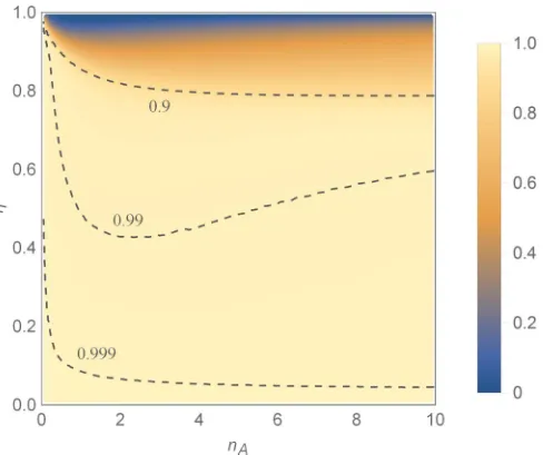
In searching for the optimal single-mode state, therefore, we fixν=1 and numerically look for the ratio|ξ|2/(2nA) that yields the largest AvQFI around a given value of(remember that the problem is-dependent in the noisy case). Intuitively, this ratio tells us the percentage of photons that we should use for displacing the state, rather than for squeezing. We plot the result in Fig.5, for 104pairs (nA,η)∈[0,10]×[0,1], for the specific example of=1. We already know that for vanishing losses (η=1) the best strategy is to squeeze the input state as much as possible, and we retrieve this feature from the

FIG. 5. Optimal value for the ratio |ξ|2_/(2n

A), leading to the maximum AvQFI value for a fixed pair (nA,η). The plot is obtained by considering=1.

plot. However, we also see that for high losses the opposite choice leads to better average performances. In particular, for a wide range of values of η below a certain nA-dependent threshold, the optimal probe can be considered a coherent state for all practical purposes (although strictly speaking a vanishingly small squeezing component is always required). In the intermediate regime, the optimal probe has a nonzero amount of both squeezing and displacement. If the value of is decreased, we obtain a similar behavior, but with a much faster transition between the two extreme regimes where the optimal parameter |ξ|2_{/(2nA) is 0 or 1 (see Appendix Gfor}

the plots associated with=0.5 or 0.1).

2. Comparison with correlated probes

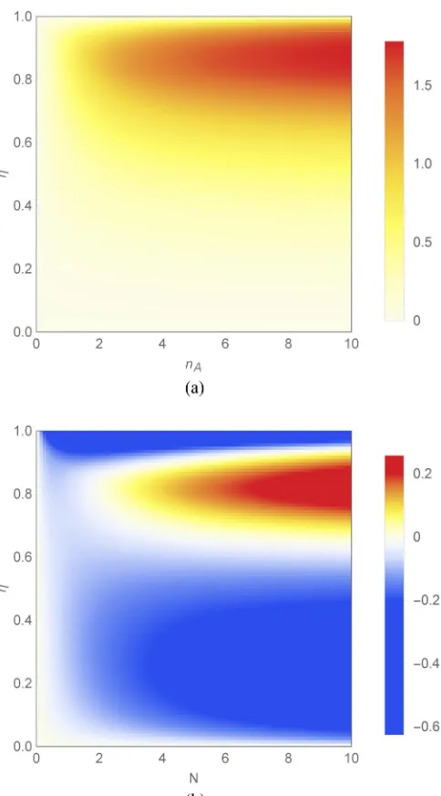
The AvQFI for the noisy encoding can be calculated for two-mode squeezed vacuum probes. This is a specific but paradigmatic choice; indeed from the results of the noiseless case we can reasonably expect that two-mode squeezed vacuum states remain optimal. The results obtained for the particular choice =1 and different values of nA (or total photon number N) and η can then be compared with the largest AvQFI obtainable by using single-mode probes with the same photon number. In Fig.6we plot the relative increase in precision that can be obtained by using this correlated input state, namely

I =H,η

ρ(sq)_AB−maxρ_AH(1)_,η(ρA)

maxρAH

(1)

,η(ρA)

, (47)

when the comparison is performed for fixednA[see Fig.6(a)] or for fixed total number of photonsN [see Fig.6(b)]. We see how two-mode squeezed states always yield a better average precision than all single-mode probes with the same nA. Remarkably, in certain conditions the same remains true even if we compare states with the same total number of photons N, thus keeping into account also the photons in the ancillary mode. For different values of the qualitative behavior is retained, but the advantageI is reduced whenis small (see AppendixGfor the plots associated with=0.5 or 0.1).

Even in presence of losses, as in the noiseless case, the QFI associated with the correlated probeρ_AB(sq)does not depend on the direction of squeezingθ applied by the device under investigation. Hence, the stability of this particular class of entangled states against fluctuations inθis not canceled by the introduction of photon losses.

IV. CONCLUSIONS

FIG. 6. Relative increaseIin precision obtained by using two-mode squeezed vacuum probes rather than the optimal single-two-mode input state, numerically evaluated for 104_{pairs (n}

A,η) or (N,η) when

=1. (a) Comparison for fixednA. (b) Comparison for fixedN.

In our analysis we analytically solved the problem for single-mode Gaussian inputs undergoing a noiseless evolution, showing that the optimal average performance can be obtained by using all the available energy to squeeze a vacuum state. However, the variance of the QFI associated with this probe necessarily increases with the photon number, potentially leading to the same precision obtainable with a vacuum input (i.e., QFI = 2) for the worst possible realization of θ. In contrast, the same average precision can be obtained with no fluctuations inθby employing a two-mode squeezed state with the same number of photons in the squeezed subsystem, at the price of doubling the total number of photons composing the probe.

We also numerically studied the same problem in presence of a noisy evolution, in which the transmission line leading

to the squeezer is affected by photon losses. We showed that, in presence of loss, the choice of using all the available energy to squeeze the input probe might not be optimal, and better average performances could be obtained by introducing a displacement along the direction of the quadrature with minimal variance. Indeed, for high losses coherent states become the optimal single-mode probe. Once the strength of the squeezing device is roughly known, the dependence of this threshold onnA can be numerically computed as in Fig.5. Finally, we numerically looked at the precision that could be reached by the paradigmatic example of two-mode squeezed states, in order to see if correlations could yield an advantage. We found that this is indeed the case, not only if the comparison is performed for fixednA, but, in some cases, also if we take into account the total photon numberN of the probe. Together with the independence of their QFI upon the squeezing direction, our results show how these states are good versatile probes, able to obtain an high estimation precision for all possible encoding realizations.

ACKNOWLEDGMENTS

L.R. thanks M. S. Kim for valuable discussions, and acknowledges financial support from the People Programme (Marie Curie Actions) of the European Union’s Seventh Framework Programme (FP7/2007-2013) under REA Grant Agreement 317232. L.A.M.S. acknowledges the Brazilian agencies CAPES (Grant No. 6842/2014-03) and CNPq (Grant No. 470131/2013-6). G.A. acknowledges financial support from the European Research Council (ERC) through the StG GQCOP (Grant Agreement No. 637352), the Royal Society through the International Exchanges Programme (Grant No. IE150570), and the Foundational Questions In-stitute (http://fqxi.org) through the Physics of the Observer Programme (Grant No. FQXi-RFP-1601).

APPENDIX A: AVQFI CHARACTERIZES THE ULTIMATE ESTIMATION PRECISION

FOR A FLUCTUATING INTERACTION

be lower bounded by

δˆ 1 MH(ρ)

, (A1)

whereM is the number of times the experiment is repeated. This result shows that the AvQFI also characterizes the ultimate precision bound attainable by a given probe in the physically relevant regime where the details of the evolution cannot be controlled, but only detecteda posteriori. When this is the case, the only viable strategy is to look at versatile probes, characterized by high AvQFI values.

In order to derive Eq. (A1) we consider a situation in which all possible probe-system interactions are labeled by an unknown parameterθ, that is also free to fluctuate from one interaction to another according to some probability p(θ). Every interaction also depends on a real parameter, that we want to estimate. In the specific example discussed in this paper, θ and represent respectively the squeezing direction and strength, whilep(θ) is taken to be uniform in [0,2π]. In what follows, we show that the weighted average of theθ-dependent QFIs characterizes the ultimate estimation precision, as long as the specific realizations ofθare known at the measurement stage.

Upon recollection of a probe, we are communicated the parameter θ that affected its evolution, and we can exploit this information to choose a suitable POVM {E(θ)

x }x. This measurement on the encoded state ρ,θ yields outcome x with probability p(x|,θ)=Tr [ρ,θEx(θ)]. Once these mea-surements have been performed on each of the M probes, we are left with a classical problem in which needs to be estimated from the knowledge ofMpairs (x,θ), sampled according to the distribution

p(x,θ|)=p(x|,θ)p(θ). (A2)

The variance of any unbiased estimator ˆcan thus be bounded via the classical Cramér-Rao bound [see Eq. (1) and Eq. (2)] associated with this probability distribution. In particular, the classical Fisher information ofp(x,θ|) is given by

F=

dx dθ p(x,θ|)[∂lnp(x,θ|)]2=

dθ p(θ)F(θ),

(A3)

whereF(θ)

is the classical Fisher information of the probability distributionp(x|,θ) obtained for fixedθ. Therefore, for any choice of POVMs this reasoning yields the bound

δˆ 1

Mdθ p(θ)F(θ)

. (A4)

Finally, notice that the right-hand side can be minimized by suitably choosing for everyθthe POVM maximizing the Fisher informationF(θ)

. Since this is exactly the optimization that defines the quantum Fisher informationH(θ)(ρ) of the probe ρ, we are left with the following ultimate bound on the variance of any unbiased estimator:

δˆ 1 MH(ρ)

, (A5)

where we defined the average QFI as

H(ρ)=

dθ p(θ)H(θ)(ρ), (A6)

by taking into account the possibility of dealing with a nonuniform distributionp(θ).

APPENDIX B: STANDARD FORM OF COVARIANCE MATRICES

We can decompose the covariance matrix and the displace-ment vector of a two-mode probe state in the following blocks:

=

_A

OFF

_OFF B , ξξξ =(ξξξA,ξξξB)

_{. (B1)}

By applying the Williamson decomposition on theB subsys-tem, one can find a local Gaussian unitary map T(B) _which

changes

B→T−1BT−1=b12, with b1, (B2)

and

OFF→OFFT−1, ξξξB →000, (B3)

while leaving subsystemAunchanged. We stress thatbis the symplectic eigenvalue of the reduced covariance matrixB, and not one of the symplectic eigenvalues of the total matrix . At this stage, thanks to the singular value decomposition (SVD), one can write

_OFFT−1=R₁Diag(c,d)R₂, (B4)

for some R₁,R₂∈SO(2) and real (not necessarily positive) parameters c,d. If R(₁A),R(₁B) are the single-mode rotations respectively associated withR₁−1,R₂−1via Eq. (16), the overall Gaussian unitary R(₁A)⊗R₁(B)◦T(B) transforms the input probe to an equivalent one that we label ρ(std)_.ρ(std) _{has the}

same average QFI of the originalρ, but the simpler structure

(std)=

⎛ ⎜ ⎜ ⎝

axaxp c 0 axpap 0 d

c 0 b 0

0 d 0 b

⎞ ⎟ ⎟

⎠, ξξξ(std)=(ξx,ξp,0,0), (B5)

and we can limit our analysis to states of this form.

For the reader familiar with the topic of quantum correla-tions in Gaussian states, we stress that this standard form is different from the one typically used when discussing Gaussian entanglement because the AvQFI is not invariant under generic Gaussian unitary operations on A.

separately.

Hdisp[ρAB]=

b|ξ|2

det[b(ax+ap)−c

2_−d2_{]. (C1)}

H[ρAB]=Hdisp[ρAB]+

c2_[4d2_−b(a

x+5ap)]+b

ba2

x+6axap+ap2−4axp2

−d2_(5a

x+ap)

2−b2_a2

xp+(c2−axb)(d2−bap)−1

−4(b

2_+cd+1)−(b2_+1)a2

xp+ax(apb2−bd2+ap)+c2(d2−bap)+cd

+[ax+b2(ax+ap)−b(c2+d2)+ap]2 2−b2_a2

xp+(c2−axb)(d2−bap)−1

axap+b2

axap−axp2 +1

−b(apc2+axd2)−a2xp+(cd+1)2

.

(C2)

APPENDIX D: SINGLE-MODE PROBES WITH MAXIMUM AND MINIMUM AvQFI

Among all single-mode probes with the same photon number nA, pure squeezed states maximize the AvQFI of Eq. (34), while thermal states minimize it. In this appendix we will formally prove this statement. Notice that if the input covariance matrix is parametrized as in Eq. (31), the AvQFI is a function of the absolute value of the input displacement|ξ| and of the quantities

Tr [A]=2νAcosh(2α), detA=ν_A2. (D1)

Let us start with the maximum. By exploiting the expression fornAgiven in Eq. (36), we can substitute the parameterαin H and obtain

H|nA =2

(2nA+1− |ξ|2)2+ν2 1+ν2 +2|ξ|

22nA+1− |ξ|2

ν2 .

(D2)

With a simple algebra, it is easy to see that the displacement has an overall negative contribution in the AvQFI expression. Therefore, if the photon-number is fixed, reducing the squeez-ing always improves the performance of the probe. We are thus left with the task of showing thatH|nAis maximized byν1 when|ξ| =0. To do so, notice that the first derivative of the function

fa,b(x)= a+x

b+x (D3)

has the same sign ofb−a. This concludes the proof because the average QFI can be written as

H|nA,|ξ|=0=2f(2nA+1)2,1(ν), (D4)

and is thus maximized by choosing the minimum symplectic eigenvalueν=1.

We now turn to the problem of finding the probe which minimizesHfor fixednA. By using Eq. (36) to substitute the value ofνin the formula for the average QFI given in Eq. (34), we find

H|nA =2(2nA+1− |ξ|

2₎2 1+cosh

2_(2α)

(2nA+1− |ξ|2)2+cosh2(2α)

+2|ξ|2cosh2(2α) 1 (2nA+1− |ξ|)

. (D5)

The first fraction appearing in this expression can be written asfa,b(cosh2[2α]) fora=1 andb=(2nA+1− |ξ|2)21. The

average QFI is then monotonically increasing with cosh(2α), and is minimized whenα=0. Finally, we have to show that the minimum H|nA,α=0 is reached for undisplaced probes. We do this by showing that its first derivative on |ξ|2 _is

always positive. After some straightforward manipulations, this inequality can be written as

√

2(Y−2X)(Y +2X)0, (D6)

where we introduced the auxiliary positive quantities

X=(2nA+1− |ξ|2), Y =

2nA+1[1+X2]. (D7)

The proof is now concluded because

Y −2X=(2nA+1−1)(1+X2)+(1−X)20. (D8)

APPENDIX E: UNIFORM SAMPLING OF SINGLE-MODE GAUSSIAN STATES

In this appendix we review the method used in Sec.III B to sample single-mode Gaussian states with fixed number of photons, uniformly distributed according to the unique invariant measure induced by the left Haar measure on the group of Gaussian unitaries. Further details on multimode generalizations can be found in Ref. [50] or references therein. Let us start with pure single-mode Gaussian states, which can be written as

ψ_G(1) ψ_G(1)=U_G(A)[|0 0|], (E1)

where |0 represents the vacuum state andUG(A) is a generic mode Gaussianity preserving unitary map. For a single-mode system we can write it as

U(A)

G =D

(A)

ξξξA ◦R

(A)

φ ◦S

(A)

α ◦R

(A)

φ , (E2)

where D_ξξξ(A)

A is the displacement map which acts on the quadraturesˆrAas

ˆrA D(A)

ξξξ A

−→ˆrA+ξξξA. (E3) With this parametrization, and using the following polar decomposition in phase space

ξξξA=(|ξ|cosψ,|ξ|sinψ), (E4)

the Haar invariant measure on the group of 1-mode Gaussian unitaries is given by

dU_G(A)= N1

2 d(coshα)dφ dφ

FIG. 7. Optimal value for the ratio|ξ|2_/(2n

A), leading to the maximum AvQFI value for 104pairs (nA,η)∈[0,10]×[0,1] and different values of. (a)=0.5. (b)=0.1.

up to a normalization constantN1. In order to impose an energy

constraint, say ofnAphotons, we can use the parametrization fornAgiven in Eq. (36) and add the Dirac delta function

δ

nA−cosh(2α)−1+ |ξ

2_|

2 . (E6)

This induces an invariant measure on the set of single-mode pure Gaussian states with fixed number of photons via Eq. (E1):

dψ_G(1)|nA =N1d(coshα)dφ dψ, (E7) with the constraint

|ξ|2=2nA+1−cosh(2α). (E8) Notice that the dependence onφdisappears because it has no effect whenUG(A)acts on the vacuum.

If we had to sample a mixed single-mode Gaussian state, we can first sample a pure two-mode state, with an approach similar to the one just described, and then apply a partial trace over one of the two subsystems. This is a standard approach in generating random mixed quantum states (see, e.g., Ref. [51]). Following Ref. [50], a pure two-mode Gaussian state can be written as

ψ_G(2) ψ_G(2)=U_G(A)⊗U_G(B)[|TMSV(ν) TMSV(ν)|], (E9)

where|TMSV(ν) is a two-mode squeezed vacuum state

|TMSV(ν) =

2 ν+1

∞

j=0

ν−1 ν+1

j/2

|j,j . (E10)

Note that the parameter ν corresponds to the symplectic eigenvalue of the reduced single-mode state obtained by tracing away the second mode. The invariant measure on the manifold of pure two-mode Gaussian states then is

dψ_G(2)= N2 3 d(ν

3_)dU(A)

G dU

(B)

G . (E11)

If modeB is traced away, the invariant measure for a mixed single-mode Gaussian state becomes

dρ_G(1)= N2N1 6 d(ν

3_{)d(coshα)d|ξ|}2_{dφ dψ, (E12)}

where we used Eq. (E5) without the irrelevant angle φ (it has no effect on a thermal state). Therefore, in order to uniformly sample a mixed single-mode Gaussian state with respect to this invariant measure, we need to (i) uniformly sampleν3,cosh(α), and|ξ|2within the region ofR3allowed by the energy constraints, and (ii) uniformly sample φ,ψ in [0,2π].

APPENDIX F: SINGLE-MODE NOISY QFI AND OPTIMAL DISPLACEMENT DIRECTION

By setting without loss of generalityφ=0 in Eq. (31), the single-modeθ-dependent QFI in the noisy case can be written as

H_,θ(1)= N1 D₁ +

N2

D₂ + N3

D₃, (F1)

where the coefficientsN₁,N₂,N₃,D₁,D₂,D₃are defined as

N1=(η−1)2η2e−4(α+){(e4α−1)ην(e4+1) cos(2θ)+4e2(α+)sinh(2)[ηνcosh(2α)−η+1]}2, (F2)

FIG. 8. Relative increase I in precision for fixed nA obtained by using two-mode squeezed vacuum probes rather than the optimal single-mode input state, numerically evaluated for 104_{pairs (n}

A,η)∈[0,10]×[0,1] and different values of. (a)=0.5. (b)=0.1.

N₃ η2 = −η

−2(e4α−1)ηνsin(4θ)ξpξx+(e4α−1)ηνcos(4θ)(ξp−ξx)(ξp+ξx)+2e2αξ_p2+ξ_x2[ηνcosh(2α)−η+1]

+2e2α(η−1) sinh(2)−cos(2θ)ξ_p2+2 sin(2θ)ξpξx+cos(2θ)ξ_x2+2e2α(η−1) cosh(2)ξ_p2+ξ_x2, (F4)

D2

2 =e

4α

(η−1)η2ν[η+cos(2θ) sinh(2)+cosh(2)]−e2α(η{η[η(ην2+η−2)+2]−2} +2η(η−1)2cosh(2)+2)

+(η−1)η2ν[η−cos(2θ) sinh(2)+cosh(2)], (F5)

D3

e2α=2(η−1)η{ηνsinh(2α) cos(2θ) sinh(2)+ηνcosh(2α)[η+cosh(2)]−(η−1) cosh(2)} +η

4_(−ν2_)−(η−1)2_(η2_+1),

(F6)

4e4(α₊)

D1

2 +1 =(e

4α₋

1)(1−η)η2ν(e4−1) cos(2θ)+2e2(α+)(2(1−η)η{ηνcosh(2α)[η+cosh(2)]

+(1−η) cosh(2)} +η4ν2+(1−η)2(η2+1)). (F7)

In particular, note that only the termN3/D3depends on the

displacement vector (ξx,ξp) of the probe, characterized by the components ξx = |ξ|cosψ andξp = |ξ|sinψ. It is possible to show that the optimal displacement direction, leading to the largest AvQFI value, isψ=π/2. In the remainder of this appendix we provide a formal proof of this statement. First, we explicitly show the dependence ofN3/D3on the anglesθ

andψby rewriting it as

N₃

D3

=x0+x1cos[2(θ+ψ)]+x2cos[2(2θ+ψ)]

x3+x4cos(2θ)

, (F8)

where the coefficients {xi}4

i₌0 depend on ,η,α, and ν; in

particular

x4=νη2(1−η)(e4α−1) sinh(2)0. (F9)

When x4=0 the dependence upon ψ disappears when we

take the average overθ. Ifx₄=0, by assuming without loss

of generality,α0, note that a comparison with Eqs. (F4) and (F6) yields the inequalities

x₁ 0, x₂ 0, x₃/x₄>1. (F10)

Then, we explicitly perform the integration of Eq. (F8) over θ∈[0,2π]. By dividing the result by 2π, we obtain the following contribution to the AvQFI:

2π

0

N3

D3

dθ 2π =

x0

2

x₃2−x₄2

+cos 2ψ 2x4

x1 2π

0

dθ 2π

cosθ x3

x4+cosθ

+x2 2π

0

dθ 2π

cos 2θ x3

x4+cosθ

, (F11)