Nonparametric series density estimation and testing

Nonparametric series density estimation and

testing

Patrick Marsh

School of Economics and

Granger Centre for Time Series Econometrics

University of Nottingham, UK, NG72RD

8th July 2018

Abstract

This paper …rst establishes consistency of the exponential series density estimator when nuisance parameters are estimated as a preliminary step. Con-vergence in relative entropy of the density estimator is preserved, which in turn implies that the quantiles of the population density can be consistently esti-mated. The density estimator can then be employed to provide a test for the speci…cation of …tted density functions. Commonly, this testing problem has utilized statistics based upon the empirical distribution function (edf), such as the Kolmogorov-Smirnov or Cramér von-Mises, type. However, the tests of this paper are shown to be asymptotically pivotal having limiting standard normal distribution, unlike those based on the edf. For comparative purposes with those tests, the numerical properties of both the density estimator and test are explored in a series of experiments. Some general superiority over commonly used edf based tests is evident, whether standard or bootstrap critical values are used.

Key words and phrases: Goodness-of-…t, Nonparametric likelihood ratio, Nui-sance Parameters and Series Density Estimator

1

Introduction

Testing whether a sample of data has been generated from a hypothesized distribu-tion is one of the fundamental problems in statistics and econometrics. Tradidistribu-tionally such tests have been constructed from the empirical distribution function (edf). Even

under the simplest of sampling schemes such tests are known to be not asymptotically pivotal, e.g. see Stephens (1976), Conover (1999) and Babu and Rao (2004). More-over, under more sophisticated sampling schemes such tests can become prohibitively complex, see Bai (2003) and Corradi and Swanson (2006).

Instead, this paper provides tests based on a generalization of the consistent series density estimator of Crain (1974) and Barron and Sheu (1991). Consistency is main-tained when nuisance parameters are estimated as a preliminary step. This, when applied to the in…nite dimensional likelihood ratio test of Portnoy (1988) generalizes

the tests of Claeskens and Hjort (2004) and Marsh (2007) to test for speci…cation. The proposed procedure o¤ers three advantages over those tests based on the edf. First they are asymptotically pivotal, and numerical experiments are designed and reported in support of this. This also implies automatic validity, including

second-order as in Beran (1988), of bootstrap critical values. Valid bootstrap critical values for the non-pivotal edf based tests, e.g. as in Kojadinovic and Yan (2012), do not bene…t from this. Second, they are generally more powerful than the most commonly used edf based tests. Again numerical evidence is presented to support this. Lastly,

because they are based on a consistent density estimator, in the event of rejection the density estimator itself can be used to, for instance, consistently estimate the quantiles of the underlying variable.

The plan for the paper is as follows. The next section presents the density

estima-tor and demonstrates that it converges in relative entropy to the population density. A corollary provides consistent quantile estimation, with accuracy demonstrated in numerical experiments. Section 3 provides the nonparametric test, establishes that it is asymptotically pivotal and consistent against …xed alternatives. A corollary

and tables containing the outcome of the experiments, respectively.

2

Consistent nonparametric estimation of possibly

misspeci…ed densities

2.1

Theoretical Results

Suppose that our sample y= _fYign_i=1 consists of independent copies of a random

variable Y having distribution, G(y) = Pr[Y y] and density g(y) = dG(y)=dy:

For this sample we …t the parametric likelihood, L =Qn_i=1f(Yi; ) for some chosen

density functionf(y; );where is an unknownk 1parameter. Denote the (quasi) maximum likelihood estimator for by ^_n:

In this context the hypothesis to be tested is:

H0 :G(y) =F (y; 0); (1)

where F (y; ) =Ry

1f(z; )dz and for some (unknown) value 0: Tests for H0 will

be detailed in the next Section. First, however, we assume the following, whether or

notH0 holds:

Assumption 1 :

(i) The density f(y; ) is measurable in y for every ₂ B, a compact subset of p dimensional Euclidean space, and is continuous in for every y:

(ii) G(y) is an absolutely continuous distribution function, E[log[g(y)] exists and _jlogf(y; )_j< v(y)for all where v(:) is integrable with respect to G(:):

(iii) Let

I( ) =E ln g(y)

f(y; ) =

Z

y

ln g(y)

f(y; ) g(y);

then I( ) has a unique minimum at some ₂B:

(iv) F (Y; )is continuously di¤erentiable with respect to , such that H( ) =

@F(Yi; )=@ is …nite, for all in a closed ball of radius >0; around :

Immediate from White (1982, Theorems 2.1, 2.2 and 3.2) is that under Assumption 1(i-iii) ^n exists and

^

n= +O(n

1=2_):

That is^_nis apnconsistent Quasi maximum likelihood estimator for the pseudo-true value : Note that under H0 we have = ₀: To proceed denote X^i =F Yi;^n

having mean value expansion,

^

Xi =F (Yi; ) + ^n

0

H + ;

where + lies on a line segment joining ^_n and . As a consequence we can write

^

Xi =Xi+ei; (2)

where Xi = F (Yi; ) and by construction and as a consequence of Assumption 1

(iv),

ei 2( 1;1) & ei =Op n 1=2 ; (3)

that is ei is both bounded and degenerate.

Since the Xi are IID denote their common distribution and density function by

U(x) = Pr X < x and u(x) = dU(x)=dx; respectively. Here we will apply the series density estimator of Crain (1974) and Barron and Sheu (1991) to consistently estimate u(x) and thus quantiles of U(x); from which the quantiles of G(y) can be consistently recovered. Application of the density estimator requires choice of approximating basis, here we choose the simplest polynomial basis, similar to Marsh

(2007).

We will approximate u(x) via the exponential family,

px( ) = exp

( _m X

k=1

kxk m

)

; _m( ) = ln

Z 1 0

exp

( _m X

k=1

kxk

)

dx; (4)

where _m( ) is the cumulant function, de…ned so thatR₀1px( )dx= 1:

Z 1 0

xkpx (m) dx= k =

Z 1 0

xku(x)dx for k = 1;2; :::; m; (5) and, as m _{! 1}; px (m) converges, in relative entropy, to u(x) at rate m 2r;

meaning that

EU

"

ln u(x)

px (m)

!#

=

Z 1 0

ln u(x)

px (m)

!

u(x)dx=O m 2r ;

asm_{! 1}:Moreover, if a sample Xi n

1 were available then ifm 3_=n

!0and letting

(m) be the unique solution to

Z 1 0

xkpx (m) dx=

Pn i=1Xik

n for k = 1;2; :::; m; (6)

then px (m) converges in relative entropy to u(x);

EU

"

ln u(x)

px (m)

!#

=

Z 1 0

ln u(x)

px (m)

!

u(x)dx=Op

m n +m

2r _;

see Theorem 1 of Barron and Sheu (1991). Here, however, the sample Xi

n

1 is not available, instead we only observe

n

^

Xi

on

1

and consequently have^(m) as the unique solution to

Z 1 0

xkpx ^(m) dx=

Pn i=1X^

k i

n for k= 1;2; :::; m: (7)

Note that the equations (5), (6) and (7) de…ne one-to-one mappings between the sample space (m) 2 Rm and the parameter space (m) 2 Rm in the

exponen-tial family, see Barndor¤-Nielsen (1978). We can therefore de…ne three pairs of

m dimensional parameter and statistics, respectively as (m) : (m) ; (m):X(m)

and n^(m) : ^X(m)

o

; where _(m) = _{f kg}m_k=1, X(m) = n 1Pn_i=1Xik m

k=1 and X^(m) =

n

n 1Pn i=1X^

k i

om k=1

: Generically these mappings can be expressed via

(m) :f kg

m

1 where

Z 1 0

xkpx (m) dx = k; k = 1; ::; m: (8)

The uniqueness of these mappings can be exploited in the following Theorem, proved in Appendix A, to show that the density estimator px ^(m) converges in

Theorem 1 Let ^(m) denote the estimated exponential parameter determined by (7)

then under Assumption 1 and for m; n_{! 1} with m3_=n

!0;

EU

2 4ln

0

@ u(x)

px ^(m)

1 A 3 5=

Z 1 0

ln

0

@ u(x)

px ^(m)

1

Au(x)dx=Op

m n +m

2r _:

According to Theorem 1, in terms of the density estimator, at least, the e¤ect

of observing nX^1; ::;X^n

o

rather than _fX1; ::; Xng is asymptotically negligible under

Assumption 1 and for either choice of basis. Moreover, if the goal were only nonpara-metric estimation of the density, then the optimal choice of the dimension m is the same as when no parameters are estimated, i.e. mopt / n

1

1+2r (with a mini-max rate

ofm_n=O n 1=5 ;since r 2by assumption). The optimal rate the rate of conver-gence of the estimator remains of orderOp n

2r

1+2r :It should not be surprising that

the rate of convergence is una¤ected when parameters are replaced bypn consistent estimators. Theorem 1 thus generalises the results of Crain (1974) and Barron and

Sheu (1991), as summarized in Lemma 1 of Marsh (2007), by permitting estimation of nuisance parameters as a preliminary step.

Additionally, we may recover the quantiles ofY from those implied by the approx-imating series density estimator. This is captured in the following Corollary, which

follows immediately since convergence in relative entropy implies convergence in law.

Corollary 1 Let T^n;m 2(0;1)be a random variable having density functionpt ^(m)

where ^(m) is de…ned by (7), then

^

Tn;m !

L X;

as n; m _{! 1}; m3=n _! 0: I.e. T^n;m converges in law to the random variable

X:

2.2

Numerical Application of a Quantile Estimator

The consequence of Corollary 1 is that the quantiles associated with Tn;m converge

to those of Y; i.e. letting qA( ); for 0 < < 1; denote the quantile function of the

random variableA; we have

q_F 1_(T^_n;m;^

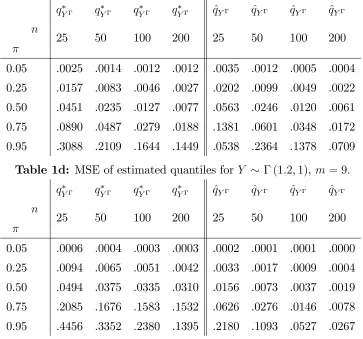
The following set of experiments compare the Mean Square Errors (MSE) of es-timators for the quantiles of Y based on those ofT^n;m for m = 3;9 and for quantiles

calculated at the probabilities, = :05; :25; :50; :75; :95. We also compare the accu-racy of estimated quantiles when unknown parameters are estimated against cases where they are not.

First suppose that Yi IID Y := t(4) but we estimate the Gaussian likelihood

implied by N( ; 2_{). De…ne}

X_i = 1

2[1 + erf (Yi)] & X^i = 1

2 1 + erf

Yi y

^ ; i= 1; ::; n;

the …rst obtained from the (misspeci…ed) Gaussian model imposing zero mean and unit variance, and the second from the Gaussian model with estimated mean and variance.

Following the development above, as well as that of Barron and Sheu (1991), let

(m) and ^(m) and denote the estimated parameters for the exponential series density

estimators for the samples _fX_ign₁ and nX^i

on

1, respectively. Let

T_n;m have density

pt (m) (note that this is just straight forward application of the original set-up of

Barron and Sheu (1991)) and letT^n;m have densitypt ^(m) ; as in Corollary 1. The

pairs of estimated quantiles for Y are then constructed as in

q_Y ( ) =p2 erf 1 2qTn;m( ) 1 and q^Y ( ) =y+ ^

p

2 erf 1 2q_T^_n;m( ) 1 :

The MSE of these quantiles, for each probability ; are presented in Appendix B, Tables 1a form = 3 and 1b form = 9:

Next suppose that Yi IID Y := (1:2;1) and de…ne

X_i = 1 e Yi _{& X}^

i = 1 e Yi=y; i= 1; ::; n:

Analogous to above let T_n;m and T^n;m have densities pt (m) and pt ^(m) and so

pairs of estimated quantiles for Y are constructed via,

q_Y ( ) = ln 1 qTn;m( ) and q^Y ( ) = ynln 1 qT^n;m( ) :

The MSE of these quantiles, for each probability ;are presented in Table 1c(m = 3)

The consistency of the quantiles obtained from, in particular, T^m;n is illustrated

clearly in Table 1. More relevant, however, is that estimating the parameters of the …tted model as a preliminary step produces quantile estimators that can be superior,

as the sample size becomes large, to those obtained by simply imposing parameter values, as can be clearly seen by comparing the right and left panels in Table 1. Note also that although the larger value of m yields more accurate quantile estimates in these cases, this is at some computational cost and, in other cases, potential numerical

instability. Although this latter possibility is greatly mitigated, since the

n

^

Xi

on i=1

are bounded.

3

Consistent, Asymptotically Pivotal Tests for

Good-ness of Fit

3.1

Main Results

Here we provide a test of the null hypothesis that the …tted likelihood is correctly

speci…ed as in (1).The previous section generalized the Barron and Sheu (1991) series density estimator and the resulting nonparametric likelihood ratio test then general-izes the test of Marsh (2007).

To proceed note that when H0 is true then in Assumption 1, = ₀ and in (2)

Xi =F (Yi; 0) IIDU[0;1]:Direct generalization of the principle in Marsh (2007)

means that (1) can be tested via,

H0 : lim

m!1 (m)= 0(m); (10)

in the exponential family (4), where (m) is the solution to (5) and 0(m) is anm 1

vector of zeros.

The likelihood ratio test of Portnoy (1988) applied via the density estimator of Crain (1974) and Barron and Sheu (1991) obtained from the sample nX^1; ::;X^n

o

is

^_{m = 2}

n

X

i=1

log

2 4pX^i

^

(m) p_X^_i 0(m)

3

The null hypothesis is rejected for large values of ^m:

Under any …xed alternative H1 : G(y) 6= F(y; 0) the distribution of Xi =

Fi(Yi; )will not be uniform, i.e. (m) 6= 0(m):For every …xed alternative distribution

for Y there is a unique alternative distribution for X on (0;1) and associated with that distribution will be another consistent density estimator given by say,px( 1(m)):In

practice, of course, 1_(m) will be neither speci…ed nor known. The following Theorem, again proved in Appendix A, gives the asymptotic distribution of the likelihood ratio

test statistic both under the null hypothesis (10) and also demonstrates consistency against any such …xed alternative.

Theorem 2 Suppose that Assumption 1 holds, we construct nX^i

on

i=1 as described in

(2), and we let m; n_{! 1} with m3_=n

!0; then: (i) Under the null hypothesis, H0 :G(y) = F(y; 0);

^_{m =} ^m m p

2m !d N(0;1):

(ii) Under any …xed alternative H1 : G(y) =6 F (y; ); for any ; and for any …nite ;

Prh^m

i

!1:

Theorem 2 generalizes the test of Marsh (2007) establishing asymptotic normality and consistency against …xed alternatives when has to be estimated. Via Claeskens and Hjort (2004) it is demonstrated that as n _{! 1} with m3_=n

! 0, then the test m (i.e. the, here, unfeasible test based on the notional sample Xi

n

1) has

power against local alternatives parametrized by (m) 0(m) = c

q_p

m

n with c0c = 1.

Heuristically, implicit from the proof of Theorem 2 the properties of the test follow from; ^m m =Op

pm

n ; and so ^m has power against that same rate of

local-alternatives.

3.2

Testing for Normality or Exponentiality

The likelihood ratio test ^m is asymptotically pivotal, speci…cally standard normal.

in Stephens (1976) or Conover (1999)) are not pivotal, although asymptotic critical values are readily available for all cases of testing for Exponentiality and Normality. First we will demonstrate that indeed asymptotic critical values for nonparametric

likelihood tests do have close to nominal size for large values of nand m: We are interested in testing the null hypotheses

H₀E :Y Exp(1) & H₀N :Y N(0;1);

with nominal signi…cance levels 10%, 5% and 1% and based on sample sizes n = 25;50;100 and 200: Letting yn and ^2n be the estimated mean and variance (i.e.

^

n =yn for H0E and ^n = yn;^2n

0

for H₀N) then the tests are constructed from the mapping to (0;1) ;

^

Xi = 1 e Yi=yn; (11)

to test HE

0 ; and

^

Xi =

1

2 1 + erf

Yi yn

^n

; (12)

to test HN

0 :

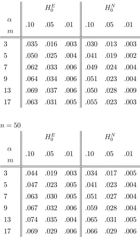
Table 2 in Appendix B provides rejection frequencies for the tests constructed for values of m = 3;5;7;9;11;17: The left hand panel of numbers correspond to testing

H₀E and the right to H₀N; critical values at the 1%, 5% and 10% signi…cance level from the standard normal distribution are used throughout.

The purpose of these experiments is only to demonstrate that the …nite sample performance of the tests clearly improves as both n and m increase, as predicted by Theorem 2(i). Note the use of three signi…cance levels to better illustrate convergence for large values of bothm and n:

Although competitor tests are not asymptotically pivotal (and therefore no

com-parisons under the null are made) instead Table 3 compares the 5% size corrected powers of two variants of the tests, with m = 3 and m = 9 with the three direct competitors for a single sample size of n = 100. Tables 3a and 3b present rejec-tion frequencies for these tests and the KS, CM and AD tests for testing HN

0 under

alternatives that the data is instead drawn from,

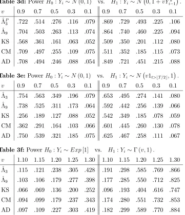
Tables 3c, 3d and 3e, consider alternatives where the moments of the data are not correctly speci…ed, i.e.

H₁c : YijYi 1 N(vYi 1;1); H₁d : YijYi 1 N 0;1 +vYi21 ; H₁e : Yi N(v 1 (i >bn=2c);1);

where 1 (:) denotes the indicator function. These latter three alternatives represent simplistic variants of common types of misspeci…cation in econometric or …nancial

data, i.e. misspeci…cation of a conditional mean, variance or the possibility of a break in the mean (here half way through the sample). Note that these models imply that (2) will not be IID on(0;1), but ergodicity implies the sample moments will still converge. Finally, table 3f considers instead testing HE

0 against the alternative

H₁f :Y (1; v):

In each table the left hand panel corresponds to the case where we construct the test imposing the parameter values speci…ed in the null rather than estimating them

(i.e. using the, unfeasible, test of Marsh (2007)). The right hand panel has the rejection frequencies for tests based on estimated values, i.e. using (11) and (12), respectively.

The outcomes in Table 3 imply the following broad conclusions. The

nonpara-metric likelihood test based ^3 is the most powerful almost uniformly, across all

al-ternatives and whether parameters are estimated or not. The observed lack of power of the most commonly used test, KS, is particularly evident, it is consistently the poorest performing test. The other edf based tests and ^9 are broadly comparable in

terms of their rejection frequencies, although AD is perhaps on average slightly more powerful and CM less powerful.

3.3

Bootstrap Critical Values

order to overcome this compromise we can instead consider the properties of these tests when bootstrap critical values are instead employed.

For these tests the bootstrap procedure is as follows: On obtaining the MLE ^_n and calculating ^3; as described above;

1. Generate bootstrap samples Yb

i IID F y; ^n fori= 1; ::; n:

2. Estimate, via ML, ^b_n and constructX^b

i =F Yib; ^ b

n for i= 1; ::; n:

3. Repeat 1 and 2 B times, obtaining bootstrap versions of the test ^b

3:

4. Order the ^b3 so the bootstrap critical value at size is B = ^b

(1 )B=100c

3 :

5. Denote the indicator function I^_B =

(

1 if ^3 > B

0 if ^3 B

)

:

We then reject H0 if I^B = 1:First, however, the required asymptotic justi…cation for

the bootstrap is automatic given that ^m !d N(0;1) giving the following corollary

to Theorem 2.

Corollary 2 Under Assumption 1 and if n; m_{! 1} with m3_=n

!0; then i) PrhI^_B = 1_jH0

i

! ;

ii) PrhI^_B = 1_jH1

i

! 1:

Here we will compare the performance of bootstrap critical values for ^3with those

of CM and AD by repeating many of the experiments of Kojadinovic and Yan (2012).

In this sub-section all experiments described in this sub-section are performed on the basis of B = 200 bootstrap replications. All nuisance parameters were estimated via maximum likelihood using Mathematica 8’s own numerical optimization algorithm.

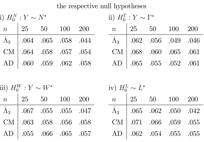
The …rst set of experiments mimic those presented in Kojadinovic and Yan (2012,

Table 1). Speci…cally we de…ne the following Normal, Logistic, Gamma and Weibull Distributions;

N N(10;1); L L(10;0:572) ;

Table 4a contains the …nite sample size of each test. It is clear that, underH0;the

parametric bootstrap provides highly accurate critical values for all of the tests. On size alone there is nothing to choose between them. It is however, worth reporting,

the computational time of each bootstrap critical value. For the ^3test critical values

were obtained after2:0and3:2seconds for sample sizesn = 100and200;respectively. The times for the other tests were similar to each other, taking around 0:9 and 2:9

seconds, respectively.

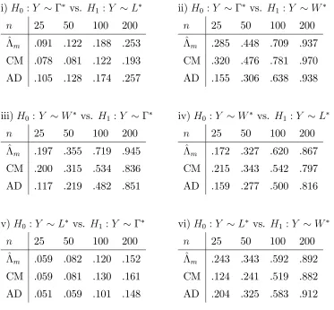
Table 4b and 4c contain the …nite sample rejection frequencies under various alternative hypotheses, covering all pairwise permutations of the distributions in (13). As with the …nite sample sizes it is not possible to pick a clear winner, moreover where they overlap the results are in line with those of Kojadinovic and Yan (2012). There

is, of course, no uniformly most powerful test of goodness-of-…t so it is not surprising that the power of ^3 is not always the largest. However its performance over this

range of nulls and alternatives is far less volatile and in no circumstance is the test dominated by any of the other two.

4

Conclusions

This paper has generalized the series density estimator of Barron and Sheu (1991) to cover the case where parameters are estimated in the context of misspeci…ed models. The nonparametric likelihood ratio tests of Marsh (2007) can be thus extended to cover the case of estimated parameters. The general aim has been to provide a testing

procedure which overcomes the three main criticisms of edf based tests, i.e. that they are not pivotal, have low power, and o¤er no direction in case of rejection.

Instead the tests of this paper are shown to be asymptotically standard normal and they have power advantages over edf tests, whether critical values are size corrected

or obtained by a consistent bootstrap. This suggests the proposed tests will be much simpler to generalize to the settings of Bai (2003) or Corradi and Swanson (2006). Finally, in the event of rejection, the series density estimator upon which the tests are built may be employed to consistently estimate the quantiles of the density from

References.

Babu, G, Rao CR (2004) Goodness of …t tests when parameters are estimated.

Sankhya 66:63–74.

Bai J (2003) Conditional Distributions of Dynamic Models. Review of Economics and Statistics 85:531-549.

Barron AR, Sheu C-H (1991) Approximation of density functions by sequences of

exponential families. Annals of Statistics 19:1347-1369.

Barndor¤-Nielsen O (1978) Information and Exponential Families in Statistical The-ory. Wiley, New York.

Beran R (1988) Prepivoting Test Statistics: A Bootstrap View of Asymptotic

Re…ne-ments. Journal of the American Statistical Association 83:687-697.

Claeskens G Hjort NL (2004) Goodness of …t via nonparametric likelihood ratios. Scandinavian Journal of Statistics 31:487-513.

Conover WJ (1999) Practical Nonparametric Statistics. Wiley, New York.

Corradi V, Swanson NR (2006) Predictive Density Evaluation. In: G. Elliott, C. Granger and A. Timmermann (eds.) Handbook of Economic Forecasting, Vol. 1, Elsevier, pp 197-284.

Crain BR (1974) Estimation of distributions using orthogonal expansions. Annals of

Statistics 2:454–463.

Kojadinovic I, Yan J (2012) Goodness-of-…t testing based on a weighted bootstrap: A fast large-sample alternative to the parametric bootstrap. The Canadian Journal of Statistics 40:480-500.

Marsh P (2007) Goodness of …t tests via exponential series density estimation. Com-putational Statistics and Data Analysis 51:2428–2441.

Portnoy S (1988) Asymptotic behavior of likelihood methods for exponential families

when the number of parameters tends to in…nity. Annals of Statistics 16:356-366. Stephens MA (1976), ‘Asymptotic results for goodness of …t statistics with unknown parameters. Annals of Statistics 4:357–369.

White H (1982) Maximum likelihood estimation of misspeci…ed models.

A

Appendix A: Proofs

In order to avoid any ambiguity throughout this appendix the order of magnitude symbol O(:)is de…ned by,

an;m =O(bn;m)() lim

m;n!1 ; m3_=n!0

an;m

bn;m

c1 <1;

and analogously for the probabilistic versions Op(:) and op(:): If the quantity

un-der scrutiny does not depend upon the dimension m then the condition m3_=n

! 0

becomes redundant.

Proof of Theorem 1:

First recall the de…nitions note ,

^

X(m) =

(Pn i=1X^

k i

n

)m

k=1

; X(m) =

Pn i=1X

k i

n 0

and _(m)=E X(m) :

The Euclidean distance between the two polynomial su¢ cient statistics satis…es,

^

X(m) X(m) =

1 n n X i=1 ^

Xi Xi ; :::; n

X

i=1

^

X_im X_im

!0 m X j=1 1 n n X i=1 ^

X_ij X_ij :

Taking the jth _{element and noting X^}

i =Xi+ei;then

1 n n X i=1 ^

X_ij X_ij = 1

n

n

X

i=1

Xi+ei j

X_ij = 1

n n X i=1 j X s=0 j!

s!(j s!)X

j s i e s i X j i = 1 n n X i=1 j X s=1 j!

s!(j s)!X

j s i e

s i:

Since Xi 2(0;1)while, as in (3), ei =Op(n 1=2)and ei 2( 1;1)then,

j!

s!(j s)!X

j s i e

s i

js

s!c

j s

1 e

s i =

js

s!c

j s

1 Op n s=2 ; (14)

where c1 <1: For …nite j (14) is Op n s=2 while as j ! 1 (14) is o(1)Op n s=2

and so,

sup

j2N

j!

s!(j s)!X

j s i e

s

implying that

j

X

s=1 j!

s!(j s)!X

j s i e

s

i =Op(n 1=2);

uniformly inj; and hence,

1 n n X i=1 ^

X_ij X_ij = 1

n n X i=1 j X s=1 j!

s!(j s!)X

j s i e

s i

!

=Op(n 1=2):

Consequently, and also from the de…nition of Euclidean distance, we have,

^

X(m) X(m) =

v u u tXm

j=1 1 n n X i=1 ^

X_ij X_ij

!2

=Op

r

m

n : (15)

Consider now _(m); then from the triangle inequality,

^

X(m) (m) X(m) (m) + ^X(m) X(m) =Op

r

m

n ; (16)

which follows from (15) and noting the same order of magnitude applies for the …rst distance, as in Barron and Sheu (1991, eq. 6.5), which represents the distance in the

case that the sequence X_ij n₁ were observed directly. We thus have X^(m) (m) = Op

pm

n and X^(m) (m) =Op

pm

n ; so that

utilizing the respective MLEs and extending the decomposition of the Kullback-Leibler divergence of Barron and Sheu (1991, eq. 6.9) we obtain,

EU

"

ln u(x)

px(^(m))

!#

= EU ln

u(x)

px( (m))

+EU ln

px( (m)) px( (m))

+EU

"

ln px( (m))

px(^(m))

!#

: (17)

Given that Assumption 1 assures the required conditions of Barron and Sheu (1991, Theorem 1) are met then the …rst two terms in (17) are, respectively, O(m 2r_{) and}

Op(m=n); noting that under Assumption 1, log[u(x)] 2 W2r. Application of Barron

and Sheu (1991, Lemma 5), which holds for any two values in m Rm;here uniquely

de…ned by equations (6) and (7), implies that

O EU

"

ln px( (m))

px(^(m))

!#!

=Op X^(m) X(m) 2

=Op

and hence

EU

"

ln u(x)

px(^(m))

!#

= O(m 2r) +Op

m

n +Op m

n

= Op m 2r+

m n ;

as required.

Proof of Theorem 2:

Consider the problem of testing H0 : (m) = 0(m) against the alternative H1 : (m) 6= 0(m) when n; m ! 1; but m3=n ! 0: For notational convenience and

com-parisons with Portnoy (1988) and Barron and Sheu (1991), expressions involving (m)

will not be immediately resolved.

Part (i): To proceed we have de…ned,

^

m = 2n ^(m) 0(m) 0

^

X(m) m ^(m) m 0(m) ;

where ^(m) solves (7), or equivalently,

0

m ^(m) =

@ _m (m) @ (m)

(m)=^(m)

= ^X(m):

Similarly the value 0(m) de…nes, 0

m 0(m) = (m)=E(X(m)):

The exponential log-likelihood is strictly convex so that the mapping, 0m (m) = (m) is one-to-one between the parameter space m Rm and sample space m

Rm_{, similar to (8). Application of Barron and Sheu (1991, eq. 5.6) and also (16) thus}

gives,

Op ^(m) 0(m) =Op X^(m) (m) =Op

r

m

n : (18)

As a consequence of both (18) and (16) we have that,

and note that the expansions provided in the provided in the proofs of Theorems 3.1 and 3.2 of Portnoy (1988) apply for any two pairs of values, here (m);0(m) and

X(m); (m) :

To continue, noting expectations under the null hypothesis can be written here asEU[:]since X U :=U[0;1], the uniform distribution with density p0(m)(x) = 1;

we then have expansions analogous to Portnoy (1988, eq. 3.5 and 3.6),

j^(m) 0(m)j2 = ^(m) 0(m) 0

^

x(m)

1

2EU0 ^(m) 0(m)

0 U

2

+Op

m2 n2 ;

and (19)

^

(m) 0(m) 0

^

x(m) = jX^(m)j2

1 2EU0

"

^

(m) 0(m) 0

U 2

^

X₍0_m)U

#

+Op

m2 n2 :

(20)

Subtracting (20) from (19) and applying arguments identical to those given below Portnoy (1988, Theorem 3.1, eq. 3.7) yields,

j^(m) (m) X^(m)j=Op

m n :

From the de…nition of the likelihood ratio test we therefore have,

^_{m = 2n} ^_{(m) 0(m)} 0_X^_(m)

m ^(m) m 0(m)

= n

"

jX^(m)j2 j^(m) 0(m) X^(m)j2+

1

6E 0 ^(m) 0(m)

0 U

3#

+Op

m2 n ;

(21)

as in Portnoy (1988, eq. 3.12). Lete= ^X(m) X(m) then from the proof of Theorem

1, we have

jX^(m)j2 =jX(m)+ej2 =jX(m)j2+Op

m

n : (22)

Now de…ne the m 1random variableVm =

00

m 0(m) 1=2

x 0_m 0(m) ;

hav-ing densitypV V(m) ;so thatE[V] = 0(m) and V ar[Vm] =Im:Since the likelihood

ratio statistic is parameterization invariant the likelihood ratio test based on obser-vations on Vm would be identical to that based on X(m): Rather than de…ning a

space m (note that in particular the hypothesized value would no longer satisfy

(m)= 0(m)) and sample space m we will instead, and without any loss of generality

assume a parameterization in which both E X(m) = 0 and V X(m) = Im: Note,

however, that it is the unobserved X which is assumed to be standardized not the observedX^(m):

In this parameterization the asymptotic distribution of …rst _jX(m)j2 and hence

jX^(m)j2 (via (22)) and then via (21) for ^m =

^_{m m} p

2m follows exactly as in Portnoy

(1988, Theorem 4.1).

Part (ii): Under any …xed alternative the density ofXi =F (Yi; ) is

u1(x) =

g(F 1(x; ))

f(F 1_{(x; ))};

and so let 1_(m) be the unique solution to,

Z 1 0

xjph 1(m) dx=

Z 1 0

hju1(x)dx ; j = 1; ::; m: (23)

The uniqueness of solutions to (23) imply 1(m) 6= 0(m):

To take the least favorable case, de…ne

1 (m)=

1 1; :

1 2; ::;

1

m

0

and suppose that 1k 6= 0 for some …nite k but that

1

j = 0 for all j 6= k: The series

density estimator is consistent for 1_(m);under H1; in that ^(m) 1(m) =Op

pm n ;

analogous to (18) above, and so we can write,

n ^(m) 0(m) 0

^

X(m) =n

"

^_(m) 1 (m)

0

^

x(m)+ 1k

1

n

n

X

i=1

k X^i

#

:

We can therefore write the likelihood ratio as

^_{m = 2n} ^_{(m) 0(m)} 0_X^_(m)

m ^(m) m 0(m)

= 2n ^(m) 1(m) 0

^

X(m) m ^(m) m

1 (m)

+2n " 1 k 0 k 1 n n X i=1 ^

X_ik _m 1_{(m) m} 0(m)

#

= ^1_m+ 2n

" 1 k 0 k 1 n n X i=1 ^

X_ik _m 1_{(m) m} 0(m)

#

where ^1_m is the likelihood ratio for testingH1 : (m) = 1(m):

Thus, under H1; we can write

^_{m =} ^m m p

2m =

^1

m m p

2m +

2nh 1_k 0_k 1_nPn_i=1X^k

i m

1

(m) m 0(m)

i

p

2m :

Immediate from Part (i) of this theorem is that asm; n_{! 1}, with m3=n_!0;

^1

m m p

2m !d N(0;1);

i.e. ^1m m = p

2m is Op(1):However, since m(:)is a uniquely de…ned cumulant

function then

m

1

(m) m

0

(m) 6= 0;

and since 0<X^i <1then _n1 Pn_i=1X^ik=Op(1) and positive. Consequently,

^

m =Op(1) +Op

n

p

m ! 1;

since m3_=n

!0and hence Prh^m >

i

B

Appendix B: Tables

Table 1: Mean Square Errors of Quantiles

Table 1a: MSE of estimated quantiles forY t(4), m= 3: q_YT q_YT q_YT q_YT q^YT q^_YT q^_YT q^_YT n

25 50 100 200 25 50 100 200

0.05 .1266 .0906 .0774 .0718 .1309 .0731 .0506 .0389

0.25 .0450 .0227 .0127 .0066 .0446 .0218 .0119 .0058 0.50 .0397 .0183 .0101 .0049 .0348 .0159 .0087 .0042 0.75 .0442 .0222 .0126 .0074 .0445 .0215 .0117 .0066 0.95 .1293 .0976 .0768 .0693 .1333 .0806 .0505 .0375

Table 1b: MSE of estimated quantiles for Y t(4),m = 9: q_YT q_YT q_YT q_YT q^YT q^_YT q^_YT q^_YT n

25 50 100 200 25 50 100 200

0.05 .1408 .1270 .1179 .1159 .1060 .0551 .0354 .0240

Table 1c: MSE of estimated quantiles for Y (1:2;1),m = 3: q_Y q_Y q_Y q_Y q^Y q^Y q^Y q^Y

n

25 50 100 200 25 50 100 200

0.05 .0025 .0014 .0012 .0012 .0035 .0012 .0005 .0004 0.25 .0157 .0083 .0046 .0027 .0202 .0099 .0049 .0022 0.50 .0451 .0235 .0127 .0077 .0563 .0246 .0120 .0061

0.75 .0890 .0487 .0279 .0188 .1381 .0601 .0348 .0172 0.95 .3088 .2109 .1644 .1449 .0538 .2364 .1378 .0709

Table 1d: MSE of estimated quantiles for Y (1:2;1),m = 9: q_Y q_Y q_Y q_Y q^_Y q^_Y q^_Y q^_Y

n

25 50 100 200 25 50 100 200

0.05 .0006 .0004 .0003 .0003 .0002 .0001 .0001 .0000 0.25 .0094 .0065 .0051 .0042 .0033 .0017 .0009 .0004 0.50 .0494 .0375 .0335 .0310 .0156 .0073 .0037 .0019

Table 2: Sizes of tests for bothHE

0 and H0N for di¤erent m and n.

n = 25

H₀E H₀N

m .10 .05 .01 .10 .05 .01

3 .035 .016 .003 .030 .013 .003 5 .050 .025 .004 .041 .019 .002

7 .062 .033 .006 .049 .024 .004 9 .064 .034 .006 .051 .023 .004 13 .069 .037 .006 .050 .028 .009 17 .063 .031 .005 .055 .023 .003

n = 50

HE

0 H0N

m .10 .05 .01 .10 .05 .01

3 .044 .019 .003 .034 .017 .005

5 .047 .023 .005 .041 .023 .004 7 .063 .030 .005 .051 .027 .004 9 .067 .032 .006 .059 .028 .004 13 .074 .035 .004 .065 .031 .005

n = 100

HE

0 H0N

m .10 .05 .01 .10 .05 .01

3 .051 .026 .004 .035 .019 .003

5 .056 .028 .006 .043 .021 .004 7 .068 .035 .008 .056 .028 .005 9 .073 .040 .007 .065 .031 .005 13 .085 .047 .008 .075 .038 .007

17 .091 .043 .009 .081 .041 .009

n = 200

HE

0 H0N

m .10 .05 .01 .10 .05 .01

3 .051 .023 .005 .045 .021 .004

5 .061 .037 .006 .053 .029 .007 7 .071 .043 .008 .063 .031 .006 9 .081 .045 .011 .078 .040 .006 13 .095 .047 .009 .086 .045 .009

Table 3: Rejection frequencies under various alternatives. The left hand pan-els corresponds parameter values imposed, while for the right had panpan-els they are estimated.

Table 3a:Power H0 :Y N(0;1) vs. H1 :Y t(v):

v 4 6 8 10 12 4 6 8 10 12

^_{3 .935 .705 .386 .267 .114 .605 .294 .166 .127 .097} ^_{9 .856 .563 .254 .159 .087 .494 .241 .133 .111 .081}

KS .614 .206 .091 .055 .049 .217 .114 .075 .059 .052 CM .722 .309 .165 .092 .061 .296 .132 .087 .075 .066 AD .767 .361 .182 .115 .065 .530 .240 .139 .103 .090

Table 3b: PowerH0 :Yi N(0;1) vs. H1 :Yi 2_(v) v:

v 12 20 28 36 44 12 20 28 36 44

^

3 .859 .660 .577 .476 .422 .572 .274 .189 .146 .114

^

9 .796 .641 .546 .427 .377 .388 .189 .158 .111 .096

KS .717 .568 .443 .388 .350 .238 .151 .106 .093 .075 CM .837 .663 .563 .463 .403 .274 .176 .131 .100 .091

AD .843 .647 .529 .439 .388 .286 .165 .117 .098 .083

Table 3c:Power H0 :Yi N(0;1) vs. H1 :Yi N(vYi 1;1): v 0.9 0.7 0.5 0.3 0.1 0.9 0.7 0.5 0.3 0.1

^

3 .694 .592 .386 .161 .093 .902 .736 .510 .271 .101

^_{9 .688 .483 .351 .141 .071 .847 .683 .461 .235 .091}

KS .592 .458 .254 .091 .053 .579 .359 .207 .122 .058

Table 3d: PowerH0 :Yi N(0;1) vs. H1 :Yi N 0;1 +vYi21 : v 0.9 0.7 0.5 0.3 0.1 0.9 0.7 0.5 0.3 0.1

^P

3 .722 .514 .276 .116 .079 .869 .729 .493 .225 .106

^_{9 .704 .503 .263 .113 .074 .864 .740 .460 .225 .094}

KS .568 .361 .161 .063 .052 .509 .350 .201 .112 .080

CM .709 .497 .255 .109 .075 .511 .352 .185 .115 .073 AD .708 .494 .246 .088 .054 .849 .721 .451 .215 .088

Table 3e: PowerH0 :Yi N(0;1) vs. H1 :Yi N v1t>bT =2c;1 : v 0.9 0.7 0.5 0.3 0.1 0.9 0.7 0.5 0.3 0.1

^_{3 .754 .563 .349 .196 .079 .653 .495 .274 .141 .080} ^_{9 .738 .525 .311 .173 .064 .592 .442 .256 .139 .066}

KS .256 .189 .127 .088 .052 .542 .349 .185 .078 .059 CM .362 .291 .164 .103 .066 .601 .445 .260 .130 .078 AD .750 .539 .321 .185 .075 .625 .467 .258 .111 .067

Table 3f:Power H0 :Yi Exp[1] vs. H1 :Yi (v;1):

v 1.10 1.15 1.20 1.25 1.30 1.10 1.15 1.20 1.25 1.30

^_{3 .115 .121 .238 .305 .428 .191 .298 .585 .769 .866} ^

9 .103 .106 .179 .277 .398 .177 .285 .550 .712 .825

Table 4a:Rejection Frequencies at 5% level under the respective null hypotheses

i) HN

0 :Y N

n 25 50 100 200

^_{3 .064 .065 .058 .044}

CM .064 .058 .057 .054 AD .060 .059 .062 .058

ii) H₀ :Y

n 25 50 100 200

^_{3 .062 .056 .049 .046}

CM .068 .060 .065 .061 AD .065 .055 .052 .061

iii)HW

0 :Y W

n 25 50 100 200

^

3 .067 .055 .055 .047

CM .063 .058 .056 .058 AD .055 .066 .065 .057

iv) HL

0 L

n 25 50 100 200

^

3 .065 .062 .050 .042

Table 4b: Rejection Frequencies at 5% level under various alternatives i)H0 :Y N vs. H1 :Y

n 25 50 100 200

^_{m .069 .088 .116 .175}

CM .078 .094 .123 .185

AD .069 .090 .108 .161

ii)H0 :Y vs. H1 :Y N n 25 50 100 200

^_{m .068 .085 .099 .129}

CM .055 .066 .079 .088

AD .076 .085 .092 .113

iii)H0 :Y N vs. H1 :Y W n 25 50 100 200

^

m .196 .364 .584 .897

CM .094 .192 .465 .776 AD .183 .315 .550 .806

iv)H0 :Y W vs. H1 :Y N n 25 50 100 200

^

m .101 .164 .351 .690

CM .107 .233 .388 .580 AD .098 .164 .334 .602

v) H0 :Y N vs. H1 :Y L n 25 50 100 200

^_{m .173 .249 .393 .458}

CM .111 .152 .212 .358

AD .131 .190 .246 .417

vi)H0 :Y L vs. H1 :Y N n 25 50 100 200

^_{m .046 .055 .065 .101}

CM .036 .054 .073 .109

Table 4c:Rejection Frequencies at 5% level under various alternatives

i)H0 :Y vs. H1 :Y L n 25 50 100 200

^

m .091 .122 .188 .253

CM .078 .081 .122 .193 AD .105 .128 .174 .257

ii)H0 :Y vs. H1 :Y W n 25 50 100 200

^

m .285 .448 .709 .937

CM .320 .476 .781 .970 AD .155 .306 .638 .938

iii)H0 :Y W vs. H1 :Y n 25 50 100 200

^_{m .197 .355 .719 .945}

CM .200 .315 .534 .836 AD .117 .219 .482 .851

iv)H0 :Y W vs. H1 :Y L n 25 50 100 200

^_{m .172 .327 .620 .867}

CM .215 .343 .542 .797 AD .159 .277 .500 .816

v)H0 :Y L vs. H1 :Y n 25 50 100 200

^

m .059 .082 .120 .152

CM .059 .081 .130 .161 AD .051 .059 .101 .148

vi)H0 :Y L vs. H1 :Y W n 25 50 100 200

^

m .243 .343 .592 .892