Classifying and modelling spiral structures in
hydrodynamic simulations of astrophysical discs
D.H. Forgan
1,2?, F.G. Ram´
on-Fox
1and I.A. Bonnell
11SUPA, School of Physics and Astronomy, University of St Andrews, North Haugh, St Andrews KY16 9SS 2St Andrews Centre for Exoplanet Science, University of St Andrews, St Andrews KY16 9SS
Submitted XXX Accepted YYY
ABSTRACT
We demonstrate numerical techniques for automatic identification of individual spiral arms in hydrodynamic simulations of astrophysical discs. Building on our earlier work, which used tensor classification to identify regions that were “spiral-like”, we can now obtain fits to spirals for individual arm elements. We show this process can even detect spirals in relatively flocculent spiral patterns, but the resulting fits to logarithmic “grand-design” spirals are less robust. Our methods not only permit the estimation of pitch angles, but also direct measurements of the spiral arm width and pattern speed. In principle, our techniques will allow the tracking of material as it passes through an arm. Our demonstration uses smoothed particle hydrodynamics simulations, but we stress that the method is suitable for any finite-element hydrodynamics system. We anticipate our techniques will be essential to studies of star formation in disc galaxies, and attempts to find the origin of recently observed spiral structure in protostellar discs.
Key words: methods: numerical, stars:formation, ISM:kinematics and dynamics
1 INTRODUCTION
Astrophysical disc structures are found across a wide range of scales – from disc galaxies to discs surrounding active galactic nuclei (AGN), to discs around protostars and even around protoplanets. Almost as commonly, these discs can be perturbed into producing spiral structures.
The means by which spiral structures are produced de-pends on the object being studied. Broadly, spiral structure is caused by some form of unstable non-axisymmetric per-turbation. How this perturbation subsequently evolves into spiral structure depends on its origin, but in most cases is caused by the disc being susceptible to gravitational insta-bility, where (for the gas) the Toomre parameter is
Q= csκ
πGΣ /1, (1)
where cs is the sound speed of the gas, κ is the epicyclic
frequency,G is the gravitational constant and Σ is the lo-cal disc surface density. A similar expression exists for the stability of a stellar disc (where the radial stellar velocity dispersion replacescs).
? E-mail:[email protected]
Spiral structures have been observed in galaxies for some 150 years, going back toRosse(1850)’s observations of M51. We now know that spiral galaxies constitute over half of observed massive galaxies (Lintott et al. 2011). This has provided theorists with significant data reserves on which to test spiral generation theories.
Spiral structures observed in disc galaxies can be self-generated, either by local instabilities/noise which are swing amplified to generate arms (e.g. Sellwood & Carlberg 1984), or through globally propagating (quasi-stationary) density waves, as predicted by the pre-eminent Lin-Shu density wave theory (Lin & Shu 1964). Spiral structures can also be exter-nally generated through tidal interactions, e.g. during galaxy mergers (Holmberg 1941’s experiments in this area are par-ticularly illuminating). Indeed, all three mechanisms (insta-bilities, density waves, interactions) can and do collaborate to produce the spiral stuctures observed both in observations and simulations (seeDobbs & Baba 2014for a detailed re-view).
Spiral arms drive important physical processes in galax-ies. Molecular clouds and recent star formation tend to be concentrated in and near spiral arms (Schinnerer et al. 2013;
Heyer & Dame 2015; Ragan et al. 2016; Schinnerer et al. 2017), most likely due to the compression and shocking of gas as it falls into the arm potential (Bonnell et al. 2006;
Dobbs & Bonnell 2007; Bonnell et al. 2013). Spiral mor-phology is also directly correlated with the surface density of neutral atomic hydrogen in the disc, and the central stel-lar bulge mass (Davis et al. 2015).
The gravitational torques induced by spiral structures will drive material into the inner few kpc of galaxies. The po-tential asymmetries caused by stellar bars can then deliver this material further inward, feeding AGN (see e.g. Alexan-der & Hickox 2012;Querejeta et al. 2016).
The wide-ranging effects of spirals on galaxy evolution has driven a great deal of effort on determining their proper-ties in observations. Attempts to characterise observed spiral structure in galaxies began with visual classification of the total number of arms, and their “openness” (Hubble 1926), which can be quantified by the pitch angleφ. The modern Hubble sequence divides spiral galaxies into barred (SB) and unbarred (S) spirals, with a further sub-class (a-d) denoting the tightness of the spiral winding.Elmegreen (1990) pro-posed dividing spirals based on their arm number (grand de-sign, multi-armed, and flocculent). More quantitative mea-surements of observed spiral galaxies involve Fourier analysis of the image (Rix & Zaritsky 1995;Foyle et al. 2010), which decomposes the azimuthal variations in surface brightness into a Fourier sum overmspiral modes with amplitudeAm,
e.g.:
µ(R, θ) ¯
µ(R) =
∞ X
m=1
Am(R)eim(θ−θm). (2)
Pitch angles can be fitted to images assuming a logarith-mic spiral of constantφ, a prediction of density wave theory (Kennicutt, R. C. 1981), or via hyperbolic spirals with ra-dially varying pitch angle (e.g.Seiden & Gerola 1979). The pattern speed of an arm can be investigated by studying star formation (and tracers of star formation) inside the arm (Egusa et al. 2004,2009). A steady arm of constant pattern speed will set up a sequence of tracers – e.g. HI, CO, 24µm emission from enshrouded stars, and UV emission from un-obscured stars – from upstream to downstream of the arm’s corotation. The failure to see this sequence in local spiral galaxies is strong evidence that spiral structures do not per-sist beyond the local dynamical time (Foyle et al. 2011).
Other observational techniques can also provide con-vincing evidence for the origin of spiral structures. For ex-ampleChoi et al.(2015) resolve the stellar populations along the northeast arm of M81, to show it does not possess a constant pattern speed. This points to a kinematic origin, driven by tidal interactions with nearby galaxies M82 and NGC 3077s.
Protostellar discs can also self-generate spiral structure through local instabilities. Shortly after the formation of a protostellar system, the protostellar disc has a mass compa-rable to that of the central star. Such discs can soon assume a marginally unstable state whereQ∼1, and the disc mass determines the spiral modes present (Lodato & Rice 2005;
Forgan et al. 2011). Interactions with a companion either internal to the disc (such as a protoplanet), or external to it (such as a close stellar encounter) also generate tidally induced spiral arms.
Spiral arms in protostellar discs are also efficient out-ward transporters of angular momentum, driving rapid
ac-cretion and assembly of protostars (Laughlin & Rozyczka 1996). Spiral structures with a sufficient surface density con-trast can concentrate dust grains (Rice et al. 2004;Clarke & Lodato 2009;Booth & Clarke 2016), promoting grain growth and setting the initial conditions for planet formation via core accretion, as well as altering local chemistry (Ilee et al. 2011;Evans et al. 2015;Ilee et al. 2017).
In extremis, spiral arms of sufficiently large density ampli-tude can induce protostellar discs to fragment into bound objects (Rice et al. 2005;Forgan & Rice 2011;Tobin et al. 2016), providing an alternate formation channel for gas gi-ants and substellar objects at large orbital semimajor axis (Forgan & Rice 2013;Forgan et al. 2015;Vigan et al. 2017). For sufficiently massive protostellar systems, fragmentation can also generate binary star systems (Bonnell & Bate 1994;
Bate et al. 2003;Tobin et al. 2016).
Spiral structure has only recently been observed in pro-toplanetary discs, initially in near-infrared (NIR) observa-tions of scattered light, which is typically most sensitive to the upper disc surface. In particular, extended two-armed structures have been detected around SAO206462 (Muto et al. 2012) and MWC 758 (Benisty et al. 2015). These arms are detectable out to relatively large distances (up to 100 au) from the parent star, with pitch angles of order 10◦. Recent ALMA observations have shown discs with spiral structure that extends down to the disc midplane, for example the re-cent detection ofm= 2 spiral structure around Elias 2-27, with a measured pitch angle of 7.9±0.4◦(P´erez et al. 2016) - the origin of this structure is not yet clear (Meru et al. 2017). Characterising these spirals, and determining their origin, yields crucial information about protostellar accre-tion and the protostar’s approach to the main sequence, as well as the formation of planetary systems.
If we are to identify the origin of newly observed pro-tostellar disc spiral structures, or to study how spiral arms govern and drive star formation in galaxies, analysing spi-ral structure driven in hydrodynamic simulations is crucial. As such, we require tools to identify and characterise spiral arms in these simulations. Regardless of scale, characteris-ing spiral morphology yields important diagnostics of what is driving the spiral structure. In particular, the number of arms, their amplitude and pitch angles are sensitive to both the driving mechanism and the disc’s properties. For ex-ample, the spiral wake produced by planets embedded in a protostellar disc adopts a pitch angle which is a function of the disc temperature and rotation profile, as well as the planetary mass (Rafikov 2002, see alsoZhu et al. 2015;Pohl et al. 2015). Gravitationally unstable discs also produce spi-ral structure with pitch angles and arm number that depend in particular on the disc mass (Dong et al. 2015), which may be a good deal larger than the observed disc mass (Forgan et al. 2016b).
Most attempts to characterise spiral structure in sim-ulations rely on Fourier decomposition (e.g. Cossins et al. 2009;Dobbs et al. 2010; Forgan et al. 2011; Mata-Chavez et al. 2014; Pettitt et al. 2016). This gives important in-formation on the relative strengths of the spiral modes at play, and the pitch angle and pattern speed of the dominant mode. However, it does not give the pitch angle and pat-tern speed of individual arms. It also does not inform us as to what sections of the disc are currently in the spiral (and which sections are in the interarm regions).
Recent attempts at spiral arm characterisation have moved away from this Fourier analysis. For example,Grand et al. (2012) attempted to directly identify individual stel-lar spiral arms in N-Body/hydrodynamic simulations of a barred spiral galaxy, by finding the location of a series of density peaks in a range of annuli. However, this does not directly provide data on the arm width, or which fluid ele-ments currently reside in the spiral.
In this paper, we demonstrate that judicious use of ten-sor classification on hydrodynamic simulation data (Forgan et al. 2016a) allows the identification of fluid elements that are inside spiral structures (or in the interarm regions). Fur-ther analysis allows the isolation of individual arms to ob-tain their shape parameters, as well as the pattern speed of the wave. Our examples focus on smoothed particle hy-drodynamics (SPH) simulations, but we emphasise that our methods only require the ability to compute derivatives, and are therefore applicable to any hydrodynamic simulation.
2 METHODS
Our spiral detection algorithm has two distinct parts. In the first part, fluid elements undergo tensor classification (Forgan et al. 2016a) to determine whether their behaviour indicates they are in fact inside a spiral structure. In the second part, the fluid elements identified as spirals are ex-tracted from the main simulation, and a friends-of-friends algorithm is used on this population to identify the spine of each individual spiral. We describe these procedures below. Our code is published on Github at https://github.com/ dh4gan/tache.
2.1 Tensor Classification
We follow the same procedure as described inForgan et al.
(2016a), which itself builds on work originally applied toN -Body simulations of the cosmic Web (see e.g. Hahn et al. 2007;Forero-Romero et al. 2009). In our formalism, tensor classification determines the topology of a chosen field at the location of a given SPH particle. We consider the topology of either the gravitational potential Φ, by computing the tidal tensorTij:
Tij= ∂2Φ ∂xi∂xj
, (3)
or the velocity field via the velocity shear tensorσij:
σij=−
1 2
∂vi ∂xj
+∂vj
∂xi
. (4)
The classification proceeds as follows. Once the tensor to be used (T or σ) is selected, its eigenvaluesλi and their
cor-responding eigenvectorsniare computed for every particle,
e.g.:
Tnj=λjnj (5)
The eigenvalues are defined soλ1≥λ2≥λ3. AsTandσare
real and symmetric, these eigenvalues are always real. Both tensors assume that the fields being investigated (potential, velocity) are smooth and continuous, so that the derivatives are always defined.
We then computeE, which is defined as the number of pos-itive eigenvalues1. The value ofE determines a topological classification for each fluid element:
• E= 0→“void” (0-D manifold)
• E= 1→“sheet” (1-D manifold)
• E= 2→“filament” (2-D manifold)
• E= 3→“cluster” (3-D manifold)
We can see this by considering the tidal tensor in the context of Zeldovich theory (Zel’dovich 1970). A test particle orbit-ing a local extremum∇Φ = 0 has the following (linearised) equation of motion:
¨
xi=−Tijxj. (6)
If we operate in a basis whereT is diagonal, then the stabil-ity of the orbit is determined by the sign of the eigenvalues
λi. A single positive eigenvalue ensures a stable orbit along
the corresponding axis (or a sheetlike structure, if multiple particles are present). Two positive eigenvalues allow an ex-tra degree of freedom (filaments) and finally all three being positive allow orbits of any degree (clusters). If no eigenval-ues are positive, stable orbits cannot be achieved (voids).
Tensor classification using the tidal tensor therefore de-termines the manifold dimension of the local potential, and as such the preferred structure for matter to collapse into if only gravity is present. Classification using the velocity shear tensor instead diagnoses the manifold being sculpted by the flow at any given instant.
As a result, the finite elements of any hydrodynamic simu-lation can be grouped into four components, with each com-ponent composed of fluid elements of a matchingE. Discs are inherently sheet-like structures, and hence perturbations from axisymmetry are classified as either filaments or clus-ters. We will see that depending on the strength of spiral structures, fluid elements classified as either filaments or clusters trace spiral structures, and that fluid elements clas-sified as sheets will trace unperturbed disc material in the interarm regions. As a general rule, the tidal tensor is bet-ter suited to tracing high-amplitude spiral structures that induce a strong surface density perturbation, but the veloc-ity shear tensor is better at revealing low-amplitude spiral structures that produce weak surface density perturbations2
1 In practice, E is defined as the number of particles whose eigenvalues exceed a small, non-zero threshold, seeForgan et al. (2016a) for details.
Tensor classification also yields eigenvectors corre-sponding to each eigenvalue. In sheets, the eigenvector n1
corresponding to the single positive eigenvalue λ1 defines
the normal or symmetry axis of the sheet. In filaments, the eigenvector n3 corresponding to the singlenegative
eigen-valueλ3 provides the flow direction of the filament. We do
not use eigenvectors in this analysis, but note that they may also be of interest in e.g. determining the relative geometry of spiral structures to their host disc.
2.2 Identifying individual spirals
Once tensor classification is complete, we extract all par-ticles that correspond to either filament or cluster classifi-cation, as these trace the spiral structure in the disc, and discard the other particles. To determine the spines of each spiral arm on this subset, we run a friends-of-friends algo-rithm as follows.
We specify a minimum spherical radius from the centre of the disc,rmin, from which to begin our study. As we are
interested in spines, we will also select the topx%percentile
in density of the remaining particles.
We then select particleiwith the largest density, where radiusri> rmin. This particle forms the first component of
the spiral’s spine.
A sphere of radiusLis then drawn fromri. The particles
inside the sphere are tested, and particlejis selected if it is the densest particle withrj > ri. Particlejthen forms the
second component of the spiral’s spine,jis then set toi, and the algorithm is repeated until a particle can no longer be found that meets the above conditions. Whenever a particle is tested, it is removed from the list of particles and is not tested again, regardless of whether it forms a component of the spiral spine or otherwise. The act of testing assigns the particle to that particular spiral. As a consequence, any particle within a distanceLof any spiral spine point belongs to that spiral.
If the conditions can no longer be met, a new spiral is begun at the location of the densest particle not yet tested, and the procedure begins again. Note that throughout we are implicitly assuming that the particle density decreases with increasing radius.
Three parameters form the identification algorithm: the linking lengthL, the minimum radius from which to begin,
rmin, and the percentile of the population from which to
conduct the analysis,x%.
The values needed for these three parameters will de-pend on the resolution and input physics of the simula-tion being analysed. The linking lengthLshould clearly be smaller than the spiral arm spacing to avoid the algorithm “jumping” between individual arms, while still being larger than the typical smoothing length to obtain a sufficient num-ber of neighbouring particles. The minimum radius should be selected based on prior knowledge of where spiral struc-ture is well-resolved (as well as the locations from which the user desires to measure said structure).
to be smooth, but it is unclear how strong discontinuities will affect tensor analysis. If reliable derivatives of a field cannot be computed for a simulation region, that region cannot be reliably classified.
The percentile selection depends on how well-defined the structures are post-tensor classification. Selecting a low
x% will result in easier classification, but will prevent the
classification of weak structures.
This algorithm delivers Nspiral sets of co-ordinate
points, with each set denoting the spine of a spiral struc-ture. We elect to fit these points via Markov Chain Monte Carlo (MCMC) to a logarithmic spiral:
r=r0+aebθ, (7)
with fit parameters (r0 = p
x2
0+y02, a, b). The origin of the
spiral is defined atθ = 0; r = r0+a. A pure logarithmic
spiral will have a constant pitch angleφ, which in radians is simply
φ= arctanb. (8) It is worth noting that if the spiral arms exclusively constitute the densest regions of our simulation, then it is likely that tensor classification will not be necessary to de-termine the location of the spiral spines, and that the above friends-of-friends algorithm will work perfectly well. How-ever, if there are other dense structures in the simulation (such as condensing clumps), then the algorithm will at-tempt to erroneously fit spiral spines to them. We have run test calculations on fragmenting discs to show that tensor classification can successfully remove dense structures that are not spiral arms, preventing this problem. Also, without tensor classification, only the spine of the arm can be deter-mined – the width of the spiral arms, or the properties of the gas contained within the arm cannot be measured.
3 TESTS
We now test our algorithm on three examples of spiral struc-ture in astrophysical discs. The origins of the strucstruc-ture in each case are subtly different. In the first, we consider a self-gravitating protostellar disc, whose spiral structure is entirely due to the self-gravity of the disc gas. In the second case, we consider a spiral galaxy with an imposed fixed po-tential that induces well-defined structures. In the last, we consider a galaxy with a “live potential” of star particles, with a resulting spiral structure that is highly flocculent.
We use smoothed particle hydrodynamics (SPH) for all three tests. SPH is a Lagrangian hydrodynamics method, where the fluid is discretised into individual particles. Each SPH particle i possesses position and velocity vectors ri,
vi, internal energy ui and smoothing length hi, which is
adjusted such that a sphere of radius 2hi encompasses a
suitable numberN of neighbour SPH particles.
The local fluid density is established by performing a sum over the neighbour particles’ smoothing kernels:
ρ(r) =
N
X
i=1
miW(|r−ri|, h). (9)
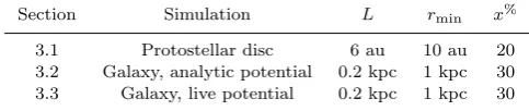
Table 1.The fit parameters used in the spiral detection algorithm for the test cases evaluated in this paper.
Section Simulation L rmin x%
3.1 Protostellar disc 6 au 10 au 20
3.2 Galaxy, analytic potential 0.2 kpc 1 kpc 30 3.3 Galaxy, live potential 0.2 kpc 1 kpc 30
the particle distribution (with appropriate compensation for shocks and fluid mixing, see Monaghan 1992, 2005; Price 2012for reviews).
Table1shows the values ofL,rmin andx%used in the
three tests run in this paper.
3.1 A self-gravitating protostellar disc
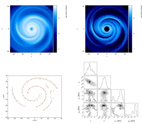
For our first test, we return to a simulation previously anal-ysed inForgan et al.(2016a). The top left panel of Figure1
shows an SPH simulation of a self-gravitating disc of mass 0.25M, orbiting a sink particle representing a star of 1M. The initial disc surface density profile follows Σ∝r−1, and
has a maximum radius of 50 au. The sound speed profile fixes the initial Toomre parameterQ= 2 at all radii.
The radiative transfer formalism ofForgan et al.(2009) is used, implementing realistic local cooling alongside typical compressive and shock heating to settle into a self-regulated, marginally stable state, where the Toomre parameterQ∼
1.5.
Marginally stable self-gravitating discs are able to sus-tain quasi-steady spiral structure for as long as the Toomre parameter can be held at this value, which depends criti-cally on the disc’s total mass, and its ability to cool. The top right panel of Figure1shows the result of tensor classi-fication using the tidal tensor. Given the deep gravitational perturbations caused by this spiral structure, we elect to use
E= 3 (cluster) particles to define the minimum potential of the structure.
The bottom row of Figure1shows the result of spiral arm identification. Bottom left shows the identified spine points of each spiral (green points), with accompanying log-arithmic fits via MCMC (red curves). An example of the derived posteriors from the MCMC fits is shown in the bot-tom right panel (for the uppermost spiral).
We see that logarithmic spirals can produce good qual-ity fits to the data, especially in the outer disc. The up-permost spiral is well fitted by a logarithmic spiral with (a, b) = (3.634±0.300,0.2468±0.0123), giving a pitch angle of 13.8◦±0.6◦. The posterior distributions fora andbare well behaved and unimodal, with only a weak degeneracy betweenaandb.
The inner radii of the spiral shows some deviation from the fit, suggesting that pitch angles may not be constant in this region. This is reflected in the best fit centre of the spiral deviating by around 1-2 au from the star’s actual position at the origin.
Repeating this analysis over a subsequent 40 timesteps of the simulation (around 1.5 outer rotation periods, Figure
2) shows that the matched spirals tend to share relatively similar parameters over this interval. The sample mean pitch
angle derived over this duration is 13.02◦, with a sample standard deviation of around 3.4◦. Interestingly, the scale parameteratends to assume slightly larger values than our example spiral, with a mean of 4.996 au, and standard de-viation 1.02 au.
Being able to measure the spiral structure over more than one timestep allows us to calculate the pattern speed of a given arm. Given that for a logarithmic spiral
θ=1
bln(r/a), (10)
we can estimate the pattern speed Ωp= ˙θgiven ˙band ˙a:
˙
θ=−b˙
b θ−
˙
a
ab. (11)
Note that ˙θ has a dependence onθonly if the pitch angle is time-dependent. Having computed ˙aand ˙bfrom the two fits, we can evaluate the pattern speed over the rangeθ= [0,2π] and take an average.
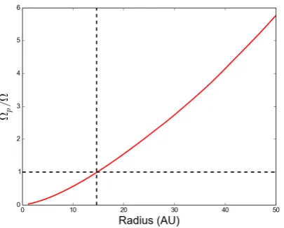
For our example spiral, we evaluate (a, b) for two snapshots and compute Ωp= 3.5×10⁻⁹rad s−1. The corotation radius,
where Ω = Ωp, is approximately 14.6 au (Figure3).
Artificial viscosity dominates the disc interior to this radius (see e.g. Artymowicz & Lubow 1994;Murray 1996;
Lodato & Rice 2004; Lodato & Price 2010; Forgan et al. 2011). The ToomreQparameter also reaches the instability regime just beyond this radius (∼20 au). As a result, the total disc stress has an artificial minimum at corotation, rather than continuing to decrease with decreasing radius (Rice & Armitage 2009).
This shows how the inner disc resolution affects the launching point of spiral structures. Indeed, unstable non-axisymmetric normal modes in self-gravitating gaseous discs are expected to trail the flow at all radii (Papaloizou & Savonije 1991).
3.2 A disc galaxy with fixed arm potential
In our second test, we use a galaxy model with analytically defined spiral structure imposed by an external gravitational potential. The galactic potential is represented by a combi-nation of an axisymmetric term plus a perturbation of the spiral arms:
Φ = Φ0+ Φpert (12)
The first component is given by a logarithmic potential (e. g.Binney & Tremaine 2008):
Φ0=
1 2v
2
0 R2+R2c+ (z/zq)2
, (13)
which has a rotation curve given by:
vc(R) =v0 R √
R2
c+R2
, (14)
wherev0 is a velocity parameter,Rc is a characteristic
ra-dius, andzq is a vertical scale factor. This produces a flat
Figure 1.Spiral arm detection in a self-gravitating protostellar disc. Top left: a snapshot from the full SPH simulation. Top right: the same snapshot, with only the SPH particles identified as exhibiting arm-like behaviour (through classification of the tidal tensor). Bottom left: the spine points of each arm (green crosses) accompanied by the best fit logarithmic spirals in red. Bottom right: The posterior distribution of the logarithmic spiral parameters for the uppermost spiral.
[image:6.595.68.511.577.741.2]Figure 3. The ratio of the pattern speed to the bulk angular velocity Ωp/Ω as a function of radius. Corotation occurs when this ratio is unity, which occurs at 14.6 au, interior to which the disc is dominated by artificial viscosity.
The velocity parameter corresponds to that of the rota-tion curve of the local spiral galaxy M33 (Corbelli & Salucci 2000;Seigar 2011;Sie Kam et al. 2015). The spiral arm per-turbation uses the scheme ofCox & G´omez(2002):
Φpert(R, θ, z, t) =
X
n
An(R, z) cos (nΓ(R, θ, t)), (15)
where An describes the perturbation amplitude which
de-cays with bothRandz(seeCox & G´omez 2002for details). Γ determines the form of spiral generated by the perturba-tion:
Γ(R, θ, t) =N
θ+ Ωpt−
ln(R/R0)
tanφ −θp
. (16)
The number of spiral armsN = 4, and their pattern speed is Ωp= 23 km s−1kpc−1 (the pitch angleφis 15◦). The
con-stantθpdefines the location of the arm at a fiducial radius R0.
The gaseous component is assumed to have an expo-nential surface density profile: Σ(R) = Σ0e−R/Rd, where Σ0
is the central surface density andRdis the scale radius. The
gas self-gravity is not included.
This analytic potential model is advantageous for its reduced computational expense, and also allows us to have a well defined spiral structure for testing the spiral detection algorithm.
Figure4 shows the full SPH simulation (top left), the particles identified as “spiral-like” using the velocity shear tensor (top right), and the particles identified as belonging to the interarm regions (E= 1, “sheet” classification, bottom left). The spines of the four main spirals are easily identified (bottom right of Figure4), and are well fitted by logarith-mic spirals each withb ≈0.25±5% (i.e. φ≈14◦±0.7◦), representing the input perturbation model well.
The separation of arm and interarm particles in azimuth is clear, if we bin particles by class in an annulus of 0.1 kpc (Figure 5). We can in fact apply Gaussian fits to the four arms to determine their angular width, resulting in a
full width half maximum (FWHM) of 0.2825 radians. This corresponds to a rather large distance of around 0.5 kpc at this radius, but this is principally due to the winding of the arms aligning them with the azimuthal vector.
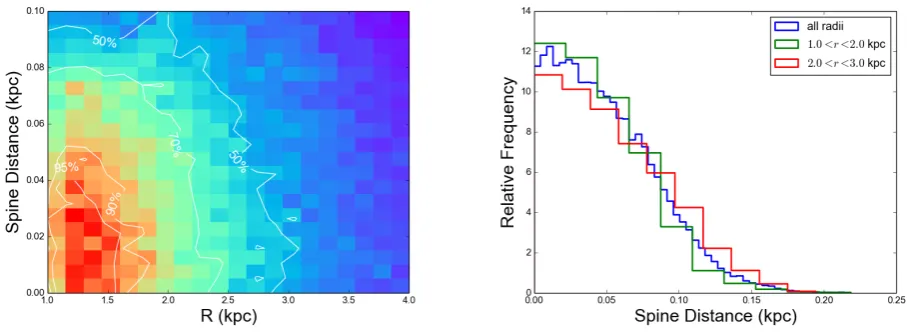
We can compute the width of a spiral arm along its entire extent by interrogating the particles that have been identified as belonging to it. We do this for the rightmost spiral in the bottom right panel of Figure4, and compute each particle’s minimum distance to the spiral spine. The left panel of Figure6shows a 2D histogram of the data (we overplot percentiles of the bin counts for convenience). We also extract 1D histograms by binning in radius (right panel of Figure6) to show that the spiral arm width is essentially constant with radius (with the FWHM of the 1D histograms being approximately 0.1 kpc).
As for the protostellar disc, we can compute pat-tern speeds by comparing two snapshots of the simula-tion. We find pattern speeds of around 20.4 km s−1kpc−1 (6.6×10⁻¹⁶rad s−1), with a 1−σ uncertainty of around
19%. Given the rotation curve, these parameters define the corotation radius as
Rco= s
v0
Ωp
2 −R2
c = 5.33 kpc (17)
The analytic spiral arm potential has a pattern speed of 23 km s−1kpc−1(7.45×10⁻¹⁶rad s−1), and corotation at 4.9 kpc. Hence, the analytic value resides within the 1−σ un-certainties of our calculation.
3.3 A disc galaxy with a live stellar potential
We also develop an N-body version of the model galaxy, which consists of a live stellar disc, a bulge and a gaseous component. The dark matter halo is represented by a static potential in order to focus the computational efforts in the disc dynamics. The stellar disc is represented by an exponential-isothermal density profile:
ρd(R, z) = Md
4πR2
dzd
exp −R Rd sech2 z zd , (18)
where Rd and zd are the radial and vertical scale lengths
respectively.
The stellar bulge follows a (Hernquist 1990) profile given by:
ρb(R) = Mb
2πR3
b
1
(R/Rb)(1 +R/Rb)3
, (19)
whereMbis the mass of the bulge andRbis the scale radius.
For the dark matter halo, a (Navarro et al. 1997) profile is used, which has a density profile of the form:
ρh(R) =
ρ0
(R/Rh)(1 +R/Rh)2
, (20)
whereRhis the scale radius andρ0 is a central density
pa-rameter. The physical parameters chosen for this model are shown in Table2, which are based on results from observed data and works modelling the rotation curve of M33 (e. g.
Regan & Vogel 1994;Corbelli & Salucci 2000;Seigar 2011;
Hague & Wilkinson 2015;Sie Kam et al. 2015)
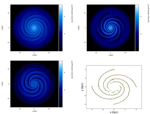
Figure 4.The evolution of a galactic disc under an analytic spiral potential. Top left: the full SPH simulation containing 2m gas particles. Top right: the particles identified as “spiral-like” (filament class). Bottom left: particles identified as moving in a disc configuration (sheet class). Bottom right: Fits to the spiral structure.
through the code mkgalaxy 3. It generates a self-consistent
model of a galaxy composed by a halo, disc, and bulge. It has the advantage of creating a stellar disc with initial ve-locities sampled from a distribution function representative of a disc rather than assuming a local Maxwellian distribu-tion in velocity space (Dehnen 1999). The disc particles have a velocity distribution consistent with the rotation curve of the galaxy. However, this code only produces a collision-less model of the galaxy and the gas initialisation has to be treated separately.
To build the full galaxy model, a disc component con-taining the total number of particles and the total combined stellar and gas mass is first generated. Then, to initialise the gaseous component, the original disc is divided into the two groups of particles and are assigned the following particle masses: mg = Mg/Ng, m? =M?/N? for the gas and
stel-lar components, respectively. At this point, the model has a gas and a stellar component, with the positions and
veloc-3 The mkgalaxy code can be obtained from the NEMO Stellar Dynamics Toolbox package (Teuben 1995) (https://bima.astro.umd.edu/nemo/).
ities obtained from the initial conditions generator. This is not an equilibrium condition for the gas itself, so the system has to be evolved for some time in order to allow it to set-tle in the galaxy. This scheme has been previously tested in
Ram´on-Fox & Aceves(2014) and a similar method also in
Dobbs et al.(2010).
Figure7shows the full simulation, its arm and inter-arm components, and fits to the spiral structure. The flocculent spiral structures are clearly identified by classification us-ing the velocity shear tensor (E = 2), but the spine fitting algorithm only outlines the larger arms with any clarity.
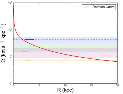
In Table3we presented calculated pitch angles and pat-tern speeds for the longest wave in the upper left and lower right quadrants the galaxy, as well as two other shorter waves in the lower left quadrant (identified by arrows in the bot-tom right panel of Figure7). The long waves yield corotation radii of approximately 1.8 and 4.2 kpc respectively (Figure
8). These values bracket the scale length of the stellar disc (Rd = 2.5 kpc), and denote the region where the rotation
curves of both the stellar and gaseous components begin to flatten, and the stellar bulge and gaseous disc enter corota-tion.
Figure 5.The number of particles classified as “arm” vs “inter-arm” in the galactic disc under the analytic potential, as a func-tion ofθ, in an annulus with inner and outer radiiR= 1.95,2.05 kpc. Also plotted are Gaussian fits to the arm histograms, with each Gaussian possessing a full width half maximum (FWHM) of 0.2825 rad. The galaxy rotates in the positiveθdirection.
appear to have much longer corotation radii (approximately 7 and 17 kpc respectively). These appear to be less robust, transient features.
4 DISCUSSION
By identifying simulation regions that are “spiral-like”, we can use the complement of these regions to identify inter-arm regions. This is a valuable distinction for studies of star formation in spiral galaxies. We can use this technique to trace the passage of a spiral shock through gas, recording the density, temperature and chemical evolution of the gas as it forms molecular clouds, and eventually stars. For ex-ample, as gas transitions from the warm diffuse phase into the dense cool phase, we will be able to time this transition relative to when the gas entered and left a spiral structure. This will be of great use in investigating the deviation of low-surface density clouds from the Kennicutt-Schmidt star formation relation (Bonnell et al. 2013), and the relation-ship in general between spiral structure and molecular clouds (Duarte-Cabral & Dobbs 2016). Spiral structure also drives amplification and reversal of the galactic magnetic field, par-ticularly at large velocity jumps over the spiral shock and at corotation (Dobbs et al. 2016). This process (of relevance to the boundness of molecular clouds) can be studied in finer detail if the fluid elements driving these magnetic amplifica-tions and reversals can be more rigorously identified.
[image:9.595.368.473.221.435.2]Being able to separate the interarm component from the arm component has its own benefits. When computing “unperturbed” disc properties, it is common to simply take azimuthal averages of the disc, and assuming the perturbed component is insignificant compared to the wider disc. If the spiral perturbation amplitude is large, this assumption fails. Being able to compute averages in the knowledge that the spiral structure has been extracted will allow a more accu-rate computation of the spiral perturbation itself (∆Σ/Σ), as well as a decontaminated study of the unperturbed disc.
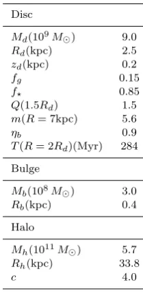
Table 2.Galaxy Model Parameters Representative of M33. The parameters are:Md- the total baryonic mass of the galactic disc;
Rd, zd- the scale length and scale height of the stellar disc;fg -the gas fraction of -the disc;f?- the stellar fraction of the disc;Q -the Toomre parameter;m- expected number of spiral modes (at given radius);ηb - the Efstathiou parameter for bar instability, which in this case is less than the critical value;T - the orbital period of the disc at a given radius;Mb- the mass of the bulge;Rb - the scale length of the bulge,Mh- the mass of the dark matter halo;Rh- the scale length of the halo;c- the halo concentration parameter.
Disc
Md(109M) 9.0
Rd(kpc) 2.5
zd(kpc) 0.2
fg 0.15
f? 0.85
Q(1.5Rd) 1.5
m(R= 7kpc) 5.6
ηb 0.9
T(R= 2Rd)(Myr) 284 Bulge
Mb(108M) 3.0
Rb(kpc) 0.4
Halo
Mh(1011M) 5.7
Rh(kpc) 33.8
c 4.0
Table 3.Fits to the four spiral arms selected from the galaxy simulation with a live stellar potential. The arms 1, 2, 3 and 4 correspond to the blue, green, orange and purple arrows in Figure 7(and similarly for the lines in Figure8). We compute uncertain-ties forRcorot by computing its value at the upper and lower 1σ limits for Ωp.
Arm φ(◦) Ωp(km s−1kpc−1) Rcorot (kpc) 1 17.59±0.87 42.57±10.59 1.82+1−0..0161 2 16.81±0.85 24.34±7.54 4.25+2−1..6241 3 13.01±0.46 7.27±0.28 17.17+0−0..8161 4 16.88±1.52 14.86±6.14 7.88+6−2..0562
Foyle et al.(2011) note that star formation rate tracers can be prominent in the interarm regions of local spiral galaxies – effective characterisation of interarm regions in simulations are needed to investigate this phenomenon, and link it to the triggering of star formation by spiral arms, as well asin situ
star formation processes.
[image:9.595.306.539.529.595.2]sys-Figure 6.The width of an individual spiral arm in the galaxy model with analytic potential, as a function of radius. Left: For a population of particles identified by our algorithms as belonging to a specific arm, we compute their minimum distance from the arm and bin them in the above 2D histogram. We overplot percentiles of the bin counts to highlight how the typical separation from an arm is constant with radius. Right: 1D histograms of distance from the arm for the same population, for all radii, and inner and outer radii.
tematic offsets due to use of the kinematic distance (Ram´ on-Fox & Bonnell 2018).
The feeding of active galactic nuclei (AGN) begins with the outward transport of angular momentum at large scales, allowing matter to flow into the inner 2-3 kpc (where stel-lar bars can take over). Lagrangian methods like SPH will be able to trace a fluid element’s journey from large dis-tances towards the nucleus, recording its encounters with spiral structure along the way.
Spiral classification has important benefits for the study of self-gravitating protostellar discs, and discs which are per-turbed by internal and external companions. In the first instance, full characterisation of a spiral arm can identify whether it is being self-generated by the disc or is due to a companion (Meru et al. 2017). Strong spiral arms in proto-stellar discs are typically induced by self-gravity, but non-axisymmetric structure can also be induced by the magneto-rotational instability (e.g.Nelson 2005). Spiral classification will provide important discriminants between the two.
Spiral arms in protostellar discs drive chemical evolu-tion (Evans et al. 2015) and potentially grain growth (Rice et al. 2004;Booth & Clarke 2016). Timing the perturbation of gas properties (and dust particles) to its passage through spiral arm passage will be critical to understanding their effectiveness.
Spiral classification is also valuable for the study of mentation in self-gravitating discs. The interaction of frag-ments with spiral arms has a significant effect on their sur-vival rate (Hall et al. 2017) and their chemical inventory (Ilee et al. 2017). Being able to observe how material is transferred between the spiral arm and the fragment will provide important insights into how fragments accrete, and how their orbital elements, physical properties and chem-istry is governed by interactions with spiral structure.
Spirals driven by companions in protostellar discs offer key diagnostics of the disc and the companion, as mentioned in the Introduction. Automatic characterisation of spirals allows simulators to run increasingly large banks of simula-tions over a wider parameter space. This opens up the
pos-sibility of potentially identifying new diagnostics from spiral arm data, as well as improved fitting of observations from grids of model runs.
Throughout this paper, we have focused on classifica-tion via a single tensor, and the choice of tensor has de-pended largely on the physics at play. In the majority of cases, where the spiral perturbation amplitude is relatively weak, spiral detection proceeds best via the velocity shear tensor (and identifyingE= 2 particles). In the limit where surface density perturbations are large, tidal tensor analy-sis is usually preferred. Our example of the self-gravitating protostellar disc is relatively extreme, in that we find best results forE= 3 particles. Our choices have reflected some knowledge of the physics of the system - the converse is equally true, that analysing using different tensors yields in-sight into the governing physics.
InForgan et al.(2016a), we showed the benefits of clas-sifying a system using multiple tensors, and then correlating the data. In an example showing the classification of struc-ture around a supernova explosion. The velocity shear ten-sor identifies regions at the inner edge of the cavity driven by the supernova; the tidal tensor identifies regions being swept into collapsing structures; correlating data identifies regions under collapse as a direct result of the supernova explosion. Spiral detection under multiple tensors can yield important information about the relative amplitudes of in-dividual arms.
[image:10.595.60.514.113.279.2]Figure 7.The evolution of a galactic disc under a live stellar potential. Top left: the full SPH simulation containing 2m gas particles, and 2m star particles. Top right: the gas particles identified as “spiral-like” (filament class). Bottom left: gas particles identified as moving in a disc configuration (sheet class). Bottom right: fits to the spiral structure. Arrows indicate four spiral arms selected for further analysis (see Figure8).
percentiles of density. We leave this as a route to follow in future work.
5 CONCLUSIONS
We have demonstrated analysis techniques that isolate and fit individual spiral arms in astrophysical disc simulations. For simulations of both protostellar and galactic discs, we are able to fit logarithmic spirals to each arm, and compute pitch angles. If multiple snapshots are available, we are also able to compute the pattern speed of spiral density waves, and identify where the wave corotates with the bulk flow.
A key innovation of these techniques is the ability to identify when fluid elements are inside a spiral structure, or in the interarm region.
Our techniques rely purely on computing derivatives of the flow at a spatial location, and the subsequent application of friends-of-friends algorithms. Therefore, our approach is applicable to data from any finite spatial element hydrody-namic solver, such as grid-based solvers using adaptive mesh
refinement, such as ENZO (Bryan et al. 2014), Voronoi mesh solvers such as AREPO (Springel 2010), or indeed meshless hydrodynamic systems such as GIZMO (Hopkins 2015). We expect our methods will prove extremely useful to simulators studying the role of spirals in the evolution of disc structures throughout the Universe.
ACKNOWLEDGMENTS
Figure 8. The rotation curve of the galactic disc under a live stellar potential, with the pattern speeds of four spiral waves marked by horizontal lines. Regions with full lines indicate the radial extent of the spiral. Dashed lines are added to illustrate the corotation radius, denoted by where the horizontal lines meet the rotation curve. Shaded regions indicate the 1−σ uncertain-ties in the pattern speed. The colours correspond with the arrow indicators in the bottom right panel of Figure7.
Our code is published on Github at https://github.com/ dh4gan/tache. The authors warmly thank the anonymous reviewer for their careful reading and astute suggestions.
References
Alexander D., Hickox R., 2012,New Astronomy Reviews, 56, 93 Artymowicz P., Lubow S. H., 1994,ApJ, 421, 651
Bate M. R., Bonnell I. A., Bromm V., 2003,MNRAS, 339, 577 Benisty M., et al., 2015,Astronomy & Astrophysics, 578, L6 Binney J., Tremaine S., 2008, Galactic Dynamics. Princeton
Uni-versity Press
Bonnell I. A., Bate M. R., 1994, MNRAS, 271, 999
Bonnell I. A., Dobbs C. L., Robitaille T. P., Pringle J. E., 2006, MNRAS, 365, 37
Bonnell I. A., Dobbs C. L., Smith R. J., 2013, MNRAS, 430, 1790 Booth R. A., Clarke C. J., 2016,MNRAS, 458, 2676
Bryan G. L., et al., 2014,ApJ, 211, 19
Choi Y., Dalcanton J. J., Williams B. F., Weisz D. R., Skillman E. D., Fouesneau M., Dolphin A. E., 2015,The Astrophysical Journal, 810, 9
Clarke C. J., Lodato G., 2009,MNRAS, 398, L6 Corbelli E., Salucci P., 2000, MNRAS, 311, 441
Cossins P., Lodato G., Clarke C. J., 2009,MNRAS, 393, 1157 Cox D., G´omez G., 2002, ApJS, 142, 261
Davis B. L., et al., 2015,ApJ, 802, L13 Dehnen W., 1999, AJ, 118, 1201
Dobbs C., Baba J., 2014,Publications of the Astronomical Society of Australia, 31, e035
Dobbs C. L., Bonnell I. A., 2007,MNRAS, 374, 1115
Dobbs C. L., Theis C., Pringle J. E., Bate M. R., 2010,MNRAS, 403, 625
Dobbs C. L., Price D. J., Pettitt A. R., Bate M. R., Tricco T. S., 2016,MNRAS, 461, 4482
Dong R., Hall C., Rice K., Chiang E., 2015, The Astrophysical Journal, 812, L32
Duarte-Cabral A., Dobbs C. L., 2016,MNRAS, 458, 3667
Egusa F., Sofue Y., Nakanishi H., 2004,Publications of the As-tronomical Society of Japan, 56, L45
Egusa F., Kohno K., Sofue Y., Nakanishi H., Komugi S., 2009, The Astrophysical Journal, 697, 1870
Elmegreen B. G., 1990,Annals of the New York Academy of Sci-ences, 596, 40
Evans M. G., Ilee J. D., Boley A. C., Caselli P., Durisen R. H., Hartquist T. W., Rawlings J. M. C., 2015,MNRAS, 453, 1147 Foreman-Mackey D., 2016,The Journal of Open Source Software,
24
Forero-Romero J. E., Hoffman Y., Gottl¨ober S., Klypin a., Yepes G., 2009,MNRAS, 396, 1815
Forgan D., Rice K., 2011,MNRAS, 417, 1928 Forgan D., Rice K., 2013, MNRAS, 432, 3168
Forgan D. H., Rice K., Stamatellos D., Whitworth A. P., 2009, MNRAS, 394, 882
Forgan D., Rice K., Cossins P., Lodato G., 2011,MNRAS, 410, 994
Forgan D., Parker R. J., Rice K., 2015, MNRAS, 447, 836 Forgan D., Bonnell I., Lucas W., Rice K., 2016a, MNRAS, 457,
2501
Forgan D. H., Ilee J. D., Cyganowski C. J., Brogan C. L., Hunter T. R., 2016b, MNRAS, 463, 957
Foyle K., Rix H.-W., Walter F., Leroy A. K., 2010,The Astro-physical Journal, 725, 534
Foyle K., Rix H.-W., Dobbs C. L., Leroy A. K., Walter F., 2011, The Astrophysical Journal, 735, 101
Grand R. J. J., Kawata D., Cropper M., 2012,MNRAS, 426, 167 Hague P., Wilkinson M., 2015, ApJ, 800, id
Hahn O., Porciani C., Carollo C. M., Dekel A., 2007,MNRAS, 375, 489
Hall C., Forgan D., Rice K., 2017,MNRAS, 470, 2517 Hernquist L., 1990, ApJ, 356, 359
Heyer M., Dame T., 2015,Annual Review of Astronomy and As-trophysics, 53, 583
Holmberg E., 1941,ApJ, 94, 385 Hopkins P. F., 2015,MNRAS, 450, 53
Hubble E. P., 1926,The Astrophysical Journal, 64, 321
Ilee J. D., Boley A. C., Caselli P., Durisen R. H., Hartquist T. W., Rawlings J. M. C., 2011,MNRAS, 417, 2950
Ilee J. D., et al., 2017, MNRAS, 472, 189
Kennicutt, R. C. J., 1981,The Astronomical Journal, 86, 1847 Laughlin G., Rozyczka M., 1996,ApJ, 456, 279
Lin C. C., Shu F. H., 1964,ApJ, 140, 646
Lintott C., et al., 2011,Monthly Notices of the Royal Astronom-ical Society, 410, 166
Lodato G., Price D. J., 2010,MNRAS, 405, 1212 Lodato G., Rice W. K. M., 2004,MNRAS, 351, 630 Lodato G., Rice W. K. M., 2005,MNRAS, 358, 1489
Mata-Chavez M. D., Gomez G. C., Puerari I., 2014, MNRAS, 444, 3756
McMillan P. J., Dehnen W., 2007, MNRAS, 378, 541
Meru F., Juh´asz A., Ilee J. D., Clarke C. J., Rosotti G. P., Booth R. A., 2017,ApJ, 839, L24
Monaghan J. J., 1992,ARA&A, 30, 543
Monaghan J. J., 2005,Reports on Progress in Physics, 68, 1703 Murray J. R., 1996, MNRAS, 279, 402
Muto T., et al., 2012,The Astrophysical Journal, 748, L22 Navarro J., Frenk C., White S., 1997, ApJ, 490, 493 Nelson R. P., 2005,Astronomy & Astrophysics, 443, 1067 Papaloizou J. C., Savonije G. J., 1991,MNRAS, 248, 353 P´erez L. M., et al., 2016, Science, 353
Pettitt A. R., Tasker E. J., Wadsley J. W., 2016,MNRAS, 458, 3990
Pohl A., Pinilla P., Benisty M., Ataiee S., Juh´asz A., Dullemond C. P., Van Boekel R., Henning T., 2015,MNRAS, 453, 1768 Price D. J., 2007,PASA, 24, 159
Querejeta M., et al., 2016,Astronomy & Astrophysics, 588, A33 Rafikov R. R., 2002,The Astrophysical Journal, 569, 997 Ragan S. E., Moore T. J. T., Eden D. J., Hoare M. G., Elia D.,
Molinari S., 2016,MNRAS, 462, 3123
Ram´on-Fox F., Aceves H., 2014, in Seigar M., Treuthardt P., eds, Structure and Dynamics of Disk Galaxies. Astronomical So-ciety of the Pacific, p. 229
Ram´on-Fox F. G., Bonnell I. A., 2018,MNRAS, 474, 2028 Regan M., Vogel S., 1994, ApJ, 434, 536
Rice W. K. M., Armitage P. J., 2009,MNRAS, 396, 2228 Rice W. K. M., Lodato G., Pringle J. E., Armitage P. J., Bonnell
I. A., 2004, MNRAS, 355, 543
Rice W. K. M., Lodato G., Armitage P. J., 2005,MNRAS, 364, L56
Rix H.-W., Zaritsky D., 1995,The Astrophysical Journal, 447, 82 Rosse E. O., 1850, Philosophical Transactions of the Royal Society
of London, 140, 499
Schinnerer E., et al., 2013,The Astrophysical Journal, 779, 42 Schinnerer E., et al., 2017,The Astrophysical Journal, 836, 62 Seiden P. E., Gerola H., 1979,The Astrophysical Journal, 233, 56 Seigar M., 2011, ISRN Astronomy and Astrophysics, 2011 Sellwood J. A., Carlberg R. G., 1984,ApJ, 282, 61
Sie Kam Z., Carignan C., Chemin L., Amram P., Epinat B., 2015, MNRAS, 449, 4048
Springel V., 2010,MNRAS, 401, 791
Teuben P., 1995, in Shaw R., Panye H., Hayes J., eds, Astronom-ical Data Analysis Software and Systems IV. AstronomAstronom-ical Society of the Pacific, p. 398
Tobin J. J., et al., 2016,Nature, 538, 483
Vigan A., et al., 2017, Astronomy & Astrophysics, 603, A3 Zel’dovich Y. B., 1970, Astronomy and Astrophysics, 5, 84 Zhu Z., Dong R., Stone J. M., Rafikov R. R., 2015,The