DOI: 10.1002/qj.3532
R E S E A R C H A R T I C L E
Comparison of the Moist Parcel-in-Cell (MPIC) model with
large-eddy simulation for an idealized cloud
Steven J. Böing
1David G. Dritschel
2Douglas J. Parker
1Alan M. Blyth
1,31School of Earth and Environment,
University of Leeds, Leeds, UK
2Mathematical Institute, University of St
Andrews, St Andrews, UK
3National Centre for Atmospheric Science,
University of Leeds, Leeds, UK
Correspondence
Steven J. Böing, School of Earth and Environment, University of Leeds, Leeds LS2 9JT, UK.
Email: [email protected]
Funding information
EPSRC (grant EP/M008525/1), NERC (grant NE/N013840/1), Met Office Academic Partnership, Royal Society, NSF (grant PHY17-48958)
Abstract
The ascent of a moist thermal is used to test a recently developed essentially Lagrangian model for simulating moist convection. In this Moist-Parcel-In-Cell (MPIC) model, a number of parcels are used to represent the flow in each grid cell. This has the advantage that the parcels provide an efficient and explicit represen-tation of subgrid-scale flow. The model is compared against Eulerian large-eddy simulations with a version of the Met Office NERC Cloud model (MONC) which solves the same equations in a more traditional Eulerian scheme. Both models perform the same idealized simulation of the effects of latent heat release and evaporation, rather than a specific atmospheric regime.
Dynamical features evolve similarly throughout the development of the thermal using the two approaches. Subgrid-scale properties of small-scale eddies captured by the MPIC model can be explicitly reconstructed on a finer grid. MPIC simulations thus resolve smaller features when using the same grid spacing as MONC, which is useful for detailed studies of turbulence in clouds.
The convergence of bulk properties is also used to compare the two models. Most of these properties converge rapidly, though the probability distribution function of liquid water converges only slowly with grid resolution in MPIC. This may imply that the current implementation of the parcel mixing mechanism underestimates small-scale mixing.
Finally, it is shown how Lagrangian parcels can be used to study the origin of cloud air in a consistent manner in MPIC.
K E Y W O R D S
clouds, convection, numerical method, thermals
1
I N T R O D U C T I O N
Detailed studies of moist convection continue to play an important role in the development of weather and cli-mate models. Such studies were initially performed using two-dimensional slab-symmetric or axisymmetric models of
clouds (e.g. Ogura, 1963). However, over the past 40 years it has become possible to run three-dimensional large-eddy sim-ulation (LES) models, which resolve the internal dynamics of clouds and the boundary layer, on increasingly large domains. LES studies form a bedrock of atmospheric research: they have been used to investigate the fine-scale dynamics
This is an open access article under the terms of the Creative Commons Attribution License, which permits use, distribution and reproduction in any medium, provided the original work is properly cited.
© 2019 The Authors.Quarterly Journal of the Royal Meteorological Societypublished by John Wiley & Sons Ltd on behalf of the Royal Meteorological Society.
of mixing between clouds and their environment (e.g. Grabowski and Clark, 1993, Heus et al., 2008), but also to aid the development of convective parametrizations (e.g. Siebesma and Cuijpers 1995) and investigate shortcom-ings of convection-permitting models (Hohenegger et al., 2015; Panosettiet al., 2016). Nevertheless, questions around fine-scale mixing remain hard to tackle because of uncer-tainty about its representation even in LES. Moreover, some research questions ask for a Lagrangian perspective: Lagrangian particles can be used in an LES model, but the representation of mixing in the model core is not fully consis-tent with the way in which particles are treated.
Existing LES models and convection-permitting models use a grid-based dynamical core, in which advection can be performed using either Eulerian or semi-Lagrangian meth-ods. In Eulerian dynamical cores, the governing equations are discretized onto an underlying mesh, and advection is performed using the discretized equations on this mesh. Semi-Lagrangian methods, on the other hand, use so-called departure points to perform advection. Within each time step, the flow from these departure points is tracked, and interpolation is used to construct the field after advection. These methods permit the use of larger time steps at the same grid resolution, but tend to violate conservation and poorly preserve correlations between tracers (Lauritzen and Thuburn, 2012). Recent work on semi-Lagrangian methods has focussed on addressing conservation issues and main-taining tracer correlations (e.g. Zerroukatet al., 2002; Kaas, 2008; Aranamiet al., 2015).
Both types of grid-based approach introduce a degree of numerical mixing: Eulerian methods because of truncation of the equations and because of the finite size of each grid box, and semi-Lagrangian methods because of the truncation and the interpolation that is performed each time step. Numerical mixing is particularly relevant for moist convection for two reasons:
1. The equation of state of moist air contains a disconti-nuity between the saturated and the unsaturated regime, which makes the problem highly nonlinear. Surprisingly, a mixture of a dry and a moist parcel can become denser than either of the two constituent parcels after its pressure adjusts to the environment (Paluch, 1979). The reason for this is the occurrence of evaporation. Numerical mix-ing and poor correlation between tracers are a cause for concern when representing such phase transitions. 2. Formation of precipitation is also highly dependent on the
highest values of liquid water that occur, again in a non-linear way. These values in turn depend on the degree of mixing in the interior of the cloud (Twomey, 1966; Blyth
et al., 2005; Cooperet al., 2013).
LESs of both cumulus (Matheou, 2011; Pressel et al., 2015) and stratocumulus (Stevens and Bretherton, 1999;
Stevenset al., 2005; Presselet al., 2015) clouds show sub-stantial sensitivities to resolution and numerical method. Both types of moist convection represent a particular challenge: for stratocumulus convection, the sharp interface at the top of the cloud layer needs to be well represented. For cumulus convec-tion, it is important to capture regions with high liquid water content where rain formation takes place, which can have a scale well below 100 m (Blythet al., 2005), as well as the dynamics of turbulent eddies and entrainment.
The aim of the current work is to test the performance of a recently developed Lagrangian model for detailed studies of moist convection. This Moist Parcel-In-Cell (MPIC) model is designed to provide a higher effective resolution in studies where convection is marginally resolved, as well as to pro-vide a more reliable, physically based approach to mixing. It differs from approaches commonly used in atmospheric mod-elling in that it represents the atmosphere through a set of parcels, rather than through a mesh-based approach. A com-panion paper (Dritschelet al.2018, hereafter D18) introduced MPIC and tested its internal consistency. Parcel-based models like MPIC have previously been used for various fluid dynam-ical problems (see the introduction of D18). MPIC also differs from most of these parcel-based approaches as it accounts for parcel buoyancy and has an explicit description of stretching of parcels at small scales.
As we expect the MPIC approach to have major benefits both in terms of computational cost and in accurately repre-senting the physics of moist convection, we perform a more detailed comparison with an LES model here. As a reference model, we use the Met Office NERC Cloud (MONC) model (Brown et al., 2015). For both models, a range of simula-tions with different resolusimula-tions is considered, including those where convection is marginally resolved, as well as simula-tions which include fine-scale turbulence deep into the inertial range.
For moist convection, a reliable description of stratifica-tion and the mixing of heat and moisture is important. D18 describe the way in which buoyancy and mixing are repre-sented in the MPIC framework. We argue that this approach has advantages for modelling cumulus convection, although further improvements may be possible. Both the development of mean properties of the cloud as well as those of turbulence and dilution on small scales are considered. The conver-gence of these properties across a range of resolutions is also tested.
2
M E T H O D O L O G Y
The test case consists of an idealized single cloud with a simplified approach to evaporation and condensation. D18 describe this case in detail. Below, we mention some key properties of the code and the test problem set-up considered.
2.1
Governing equations
We use a simplified set of governing equations introduced in D18. The governing equations for velocityu, liquid water buoyancy𝑏𝑙and specific humidity𝑞are
Du D𝑡 = −
𝜵𝑝 𝜌0
+𝑏̂e𝑧, (1)
D𝑏𝑙
D𝑡 =0, (2)
D𝑞
D𝑡 =0, (3)
𝜵⋅u=0, (4)
where D∕D𝑡=𝜕∕𝜕𝑡+u⋅𝜵represents a material derivative. In Equation 1 the total buoyancy𝑏(including the effects of latent heating) is approximated by
𝑏=𝑏𝑙+ 𝑔𝐿 𝑐𝑝𝜃𝑙0𝑞𝑙,
(5)
where
𝑞𝑙 =max(0, 𝑞−𝑞0e−𝜆𝑧 )
(6)
is the liquid water content. The pressure 𝑝 in Equation 1 excludes the part due to the hydrostatic background state of constant density 𝜌0. The other symbols appearing in Equations 1–6 are the vertical unit vector̂e𝑧, the gravitational acceleration𝑔, the latent heat of condensation𝐿, the specific heat at constant pressure𝑐𝑝, the surface saturation humidity
𝑞0, and the inverse condensation scale height𝜆. The liquid water buoyancy is defined by𝑏𝑙=𝑔(𝜃𝑙−𝜃𝑙0)∕𝜃𝑙0, where 𝜃𝑙 is the liquid water potential temperature and𝜃𝑙0is a constant reference value.
2.2
Parcel-based model
As discussed in D18, the parcels in the MPIC model carry liquid water buoyancy𝑏𝑙, specific humidity𝑞, parcel volume
𝑉 and vorticity𝝎. The prognostic equation for vorticity reads
D𝝎
D𝑡 =𝝎⋅𝜵u+ (
𝑏𝑦,−𝑏𝑥,0), (7)
where subscripts on𝑏 denote spatial partial differentiation. The velocity field is needed both to evolve the positions of the parcels as well as to calculate the right-hand side of the
vorticity equation. D18 discuss the use of tri-linear interpo-lation on a grid to obtain a Poisson equation for the gridded velocity field given the gridded vorticity field. The different scale of the advecting velocity field compared to the particle size resembles a similar effective distinction made in layer-wise two-dimensional contour advection methods (Dritschel and Ambaum, 1997; Fontane and Dritschel, 2009).
Particle-mesh methods typically treat fluid elements as indivisible. This is not a suitable approach for the simula-tion of clouds, as mixing is needed on longer time-scales in order to represent the eventual evaporation of the cloud, which occurs at the end of the process of turbulent mixing. MPIC contains an explicit representation of the stretching and eventual mixing of parcels, detailed in D18. The amount of stretching that a parcel has experienced is prognostically calculated, and when this exceeds a critical threshold, a par-cel is split. The choice of threshold value is also related to the assumed distance between parcels after splitting (D18). When this splitting leads to the parcel becoming smaller than a critical volume (here 1∕216 of the grid box volume), the parcel properties are merged with those of surrounding parcels through operations on the grid, using the conservative method developed in D18. D18 considered the sensitivity to the threshold; they found limited sensitivity over a wide range of values.
Another key numerical advantage of our approach is that buoyancy in Equation 5 is calculated at the level of each indi-vidual parcel, before it is summed to grid-based values. The order of these operations implies that nonlinearities in the thermodynamics are retained (Tsang and Vallis, 2018).
2.3
Non-dimensionalization
As discussed in D18, the equations are non-dimensionalized by setting the length-scale 1∕𝜆=1 in Equation 5. The char-acteristic squared buoyancy frequency 𝑔𝜆Δ𝜃𝑙0∕𝜃𝑙0 = 1 is used to non-dimensionalize time. Here,Δ𝜃𝑙0∕𝜃𝑙0= 0.01 is a characteristic fractional variation of the liquid water potential temperature. This gives a dimensionless gravity of𝑔 =100. The specific humidity𝑞is scaled by its saturation value𝑞0at ground level (i.e. we usẽ𝑞=𝑞∕𝑞0in what follows). We obtain the following dimensionless expression for the buoyancy𝑏:
𝑏=𝑏𝑙+𝑏mmax (
0, ̃𝑞−e−𝑧), (8)
where
𝑏m= 𝑔𝐿𝑞0
𝑐𝑝𝜃𝑙0 .
(9)
that is, an anelastic formulation; this option is not used in the present work. A rough estimate of the length-scale𝜆in the atmosphere is that it is of the order 2 km, which would make the domain 12 km high and the grid spacing in the 2563 simu-lation about 50 m. In this case, some of the other assumptions we have made such as a lack of precipitation and a Boussi-nesq approach are not valid. The boundary layer would also be much deeper than is typical for an atmospheric case.
Alternatively, we can think of our simulation as a more shallow cloud, but with stronger saturation specific humidity dependence on temperature than in the atmospheric case. This means convection will be more vigorous than in atmospheric shallow convection.
Possibly, scaling all heights that define the case by a fac-tor of about1∕3to1∕2with respect to𝜆would have been a good
choice, as this would make them characteristic of shallow con-vection over land. The main reason we chose the parameters in the way we have done is that these allow us to test the dynamics with a strong nonlinearity across a range of resolu-tions. In summary, the set-up can be thought of as a thermal which releases a substantial amount of latent heat, rather than a realistic cloud in a particular atmospheric regime.
2.4
Case description
The different models are compared using a moist buoyant thermal which is initially at rest and located near the sur-face. The thermal first rises through a neutrally stable lower atmospheric layer before encountering a layer with a constant stratification aloft. In order to prevent the flow from being overly symmetric, the buoyancy field in the spherical interior of the thermal is initialized as:
𝑏𝑙=𝑏𝑙th (
1+𝑒1𝑥 ′𝑦′+𝑒
2𝑥′𝑧′+𝑒3𝑦′𝑧′
𝑅2
)
. (10)
Here,𝑏𝑙this the mean thermal liquid water buoyancy, and
𝑥′, 𝑦′ and 𝑧′ denote the position with respect to the
ther-mal centre and𝑅the thermal radius, while𝑒1,𝑒2 and𝑒3are dimensionless parameters. These parameters are chosen as
𝑅 = 0.8, 𝑒1 = 0.3,𝑒2 = −0.4 and𝑒3 = 0.5. The top of the neutrally stratified layer is located at𝑧 ≈ 2.38 and the dimensionless Brunt–Väisälä frequency above is𝑁 ≈ 0.97. The environment relative humidity is set to 80% at all levels in the stratified layer, and the specific humidity is constant in the neutrally stratified layer, with a value chosen such that there is no discontinuity at the top of this layer. This value is also 90% of the specific humidity in the thermal.
A full overview of the procedure and parameters used to construct the parcel properties is given in D18. In MONC, the same procedure is used, but the specific humidity and buoy-ancy are initialized at the relevant locations on the (staggered) grid, rather than on parcels.
The reason for using a warm and moist thermal is that the detailed flow evolution can be compared across models and resolutions not only on a statistical basis, but also directly. Recently, we have made a number of changes to the solver which enable us to use a non-zero buoyancy gradient at the boundary. This will help us to implement boundary condi-tions that are suitable for real-case atmospheric simulacondi-tions in future work.
The moist thermal has asharpedge, that is, there is a dis-continuity of buoyancy at the edge. This has the drawback that it is less realistic and leads to vorticity values which depend on resolution. In general, our results are likely to be more sen-sitive to resolution than simulations with a smoother initial thermal edge. However, the advantages of this approach are that it makes it easier to track the parcels that are defined as the initial thermal, and it accelerates the transition from rest to a fully turbulent flow.
2.5
MONC simulations
MONC is a LES model that has been developed for research on atmospheric boundary layers and clouds. The model for-mulation of MONC follows that of its predecessor, the Met Office Large-Eddy Model, which has been used for many years for atmospheric process studies and LES intercompar-ison studies (e.g. Petch and Gray, 2001; Abel and Shipway, 2007). However, the code has been completely rewritten for use on modern parallel computing architectures (Brownet al., 2015).
In the MONC simulations, the same idealized thermo-dynamics are used as in the MPIC simulations and we have adapted the model formulation and set-up (domain size and thermodynamics) to match that of MPIC. The model integrates prognostic equations for the different com-ponents of the momentum equation and the scalars 𝑏𝑙 and
𝑞 on a grid with Arakawa C-staggering. For scalars, it uses the positivity-preserving ULTIMATE advection scheme (Leonard et al., 1993). For the advection of momentum and the subfilter-scale fluxes, we consider two different approaches in this work.
1. MONC-Smagorinsky: Velocity components are advected using a second-order kinetic energy conserving scheme (Piacsek and Williams, 1970). Hence there is a need for subgrid-scale dissipation: subfilter-scale fluxes of scalar quantities and momentum are determined using the Smagorinsky approach (Smagorinsky, 1963). Effects of stratification are taken into account in the determination of the eddy viscosity, as they are in the default version of MONC.
unsaturated air, we define the Richardson number as𝑅𝑖 = (𝜕𝑏𝑙∕𝜕𝑧)∕𝑆. Here,𝑆is the modulus of the rate of strain tensor. For saturated air, a correction is made for latent heat release:
𝑅𝑖= (𝜕𝑏𝑙∕𝜕𝑧+𝑏me−𝑧) ∕𝑆.
2. MONC-Implicit: velocity components are advected using the ULTIMATE advection scheme, and no explicit subgrid-scale model is used. This approach is referred to as implicit LES.
The pressure is determined diagnostically using a Poisson equation, which is solved using Fast Fourier Transforms in the horizontal and a tridiagonal solver in the vertical. MONC was run with a constant time stepΔ𝑡, proportional to the grid spacingΔ𝑥, namelyΔ𝑡 =0.2Δ𝑥∕𝜋. We have used a constant time step in MONC as this was the easiest way to obtain output at (or near) the exact time when it was required with MONC’s IO-server.
We take the grid spacing to be the same in 𝑥, 𝑦 and
𝑧. Horizontal boundary conditions are doubly periodic. Free-slip boundary conditions are used at both domain bot-tom and domain top for horizontal momentum, whereas for temperature and moisture, the flux at the boundaries is set to zero.
2.6
Use of subgrid-scale diagnostics for
MPIC
For MPIC, we mostly show results that have been obtained by post-processing the particle information using a finer grid. MPIC uses a large number of parcels per grid box (typically 10–200), each of which occupies only a small fraction of the grid box volume. This means that gridded quantities fail to show the actual variability below grid scale that is present in the model. In order to visualize this subgrid variability, a pro-jection algorithm is employed that works with a representative radius for each parcel. A full description of the projection algorithm can be found in Appendix A.
For computing statistics of the liquid water field in MPIC, we make use of the direct statistics of parcels. Appendix B discusses how the probability distribution function of liquid water depends on the method used to compute it.
2.7
Computational cost
In the following, the number of grid points is mentioned in comparisons between MPIC and MONC. However, a like-for-like comparison is not easy to infer, since MPIC exploits the existence of many parcels within each grid box. Although the computational cost of the solver is largely deter-mined by the number of grid points, the total computational cost is harder to compare.
MPIC was run using shared-memory parallelism (OpenMP) for this study. This is the reason that the maximum
number of grid points used was limited to 3843, whereas for MONC, which uses MPI parallelism, 10243points could be used. In the meantime, a project to produce a hybrid parallel (OpenMP+MPI) version of MPIC in collaboration with the Edinburgh Parallel Computing Centre, which uses MONC’s infrastructure, is close to being finished.
The number of parcels plays an important role in the cost of MPIC simulations, even though parcel operations are relatively straightforward. Parcel operations (including inter-polation of values to and from the grid) are responsible for the bulk of the cost of the MPIC simulations (79% for par-cel operations and 9% for parpar-cel time stepping in a 1283grid points simulation). The FFT operations are responsible for about 10% of the computational cost.
The simulation with 2563grid points took approximately 99 core hours (the number of hours spent multiplied by the number of computational units involved) on ARCHER for MONC and 751 core hours on a local machine for MPIC using 24 cores. The OpenMP-only parallelism does not scale perfectly: as an example, for a 1283 grid point simulation on eight cores the speed-up was a factor 5.35 compared to a sin-gle core, whereas using 24 cores only resulted in a speed-up of a factor 8.17. Early results from the hybrid parallel ver-sion on ARCHER show a total runtime of 453 core hours on 128 cores, with 17% of this time spent on FFT operations. The latter is a greater fraction of computational cost, but the total time spent on FFTs is similar to that in the version with shared-memory parallelism only. We aim to further optimize the relative cost of parcel and grid operations in future work. The number of time steps for the computation with 2563 grid points is 1667 for MPIC and 6400 for MONC. However, MPIC uses an RK4 time-integration scheme, whereas MONC uses a leap-frog approach with an Asselin filter. In MPIC, the solver is called four times per time step, so effectively the number of calls to the solver is similar. We have followed a relatively conservative approach in choosing the time step for both models. The time step length in MPIC mainly changes during the initial phase, and the smallest time step of 0.0039 time units occurs at𝑡=5.92.
3
R E S U L T S
3.1
Evolution of the flow at high resolution
F I G U R E 1 Cross-sections of dimensionless liquid water specific humidity𝑞𝑙, for (a, b, c) MPIC, and for MONC with (d, e, f) a Smagorinsky and (g, h, i) an implicit subgrid formulation after (a, d, g) 4, (b, e, h) 6 and (c, f, i) 8 time units
important to keep in mind that, for producing Figure 1 and the detailed cross-sections shown in Figure 2, the MONC simula-tions had a much higher total computational cost. The number of parcels in the MPIC simulation is larger than the number of grid points by a factor of 8 at the start of the simulation, which increases to a factor of 16 at the end. The MPIC results are rendered using the algorithm described in Appendix A.
The large-scale evolution of the thermal is similar between the models, and even some of the smaller-scale features that arise due to the initial asymmetry are comparable at𝑡 = 8. Closer inspection also shows that, at𝑡 = 6, the thermal in MPIC has ascended further than the one in MONC.
MPIC shows a very large amount of fine-scale structure at the reference resolution, whereas the liquid water field looks relatively smooth in MONC, particularly for the Smagorinsky model. This is even more evident in the detailed cross-sections shown in Figure 2. In this figure, the MPIC results are also shown averaged to the coarse grid used in the dynamics. Some of the detail in the liquid water field (left column) is lost when only the grid-scale properties are used for visualization.
Larger differences between the reference simulations occur in the vorticity and velocity fields. The magnitude of the vorticity vector is shown in Figure 2b,e,h,k. MPIC shows a sharply confined region of high vorticity with a large amount of structure (in particular, it includes long swirling features), whereas in MONC the filaments are broken into multiple seg-ments and are less confined. We will address the extent to which this depends on resolution below.
(a) (b) (c)
(d) (e) (f)
(g) (h) (i)
(j) (k) (l)
ql
F I G U R E 2 Detailed zoom into (a, d, g, j) the liquid water specific humidity𝑞𝑙, (b, e, h, k) vorticity and (c, f, i, l) vertical velocity fields in the most active part of convection at𝑡=6. For MPIC, both results using (a, b, c) the method in Appendix A and (d, e, f) at the scale of the grid are shown. MONC uses either (g, h, i) the Smagorinsky subgrid scheme or (j, k, l) an implicit LES formulation
to the vorticity tendency equations, but this is currently not done (as parcels are advected with the gridded velocity fields in any case).
The vertical velocity shown in Figure 2f,i,l shows less structure in the MPIC fields than in the MONC ones. This is to be expected as this variable only exists on the grid, which is three times coarser for MPIC than for MONC.
In conclusion, the large-scale evolution of the thermal is similar in the two reference simulations. MPIC contains more small-scale features in the liquid water and vorticity fields, though the velocity field at the grid scale shows more
fine-scale structure in MONC, which uses a larger number of grid points.
3.2
Resolution sensitivity of the flow
evolution
F I G U R E 3 Cross-sections of liquid water specific humidity at𝑡=6 using (a, b, c) 163to (j, k, l) 1283grid points, for (a, d, g, j) MPIC, and for
MONC with (b, e, h, k) Smagorinsky and (c, f, i, l) implicit subgrid formulation
with the same grid spacing; admittedly, the computational cost at this grid spacing is currently higher for MPIC than for MONC.
Two differences between the MONC and MPIC simu-lations are clear. First, the coarsest MONC simusimu-lations are overly diffusive as compared to the high-resolution reference simulations. Intermediate MONC simulations preserve the maxima in the liquid water field better. MPIC, on the other hand, may be underdiffusive when the flow is marginally resolved, as can be seen by comparing the buoyancy fields in a low- and an intermediate-resolution simulation
(Figure 4); a significant local maximum in buoyancy occurs in the vortex ring in the low-resolution MPIC simulations, whereas this maximum is much less pronounced at higher resolutions.
The differences between MPIC and MONC are more read-ily apparent at later times, when diffusive effects accumulate in MONC. This is shown in Figure 5, for the condensed por-tion of the specific humidity (comparing times 𝑡 = 4 with
F I G U R E 4 Cross-sections of buoyancy after 6 time units for simulations using (a, b, c) 323and (d, e, f) 1283grid points. Columns are as in
Figure 3
F I G U R E 5 Time evolution of liquid water specific humidity in the simulations using 643grid points after (a, b, c) 4 time units and (d, e, f) 8
time units. Columns are as in Figure 3
and gradually evaporates. Turbulent motions are better repre-sented in the MPIC model than in MONC, and are sustained in time.
Both models capture the same intermediate and large-scale features when used across a range of resolutions. However, the
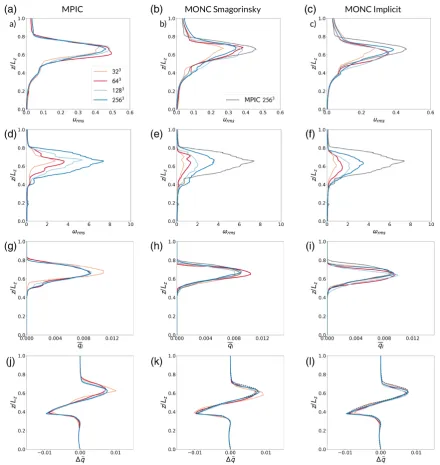
F I G U R E 6 Resolution sensitivity of bulk flow properties at𝑡=6: (a–c) root-mean-square velocity, (d–f) root-mean-square vorticity and (g–i) liquid water specific humidity. (j–l) show the difference in total specific humidity between the start and end of the simulations. Columns are as in Figure 3. Colours represent the number of grid points (323pink, 643red, 1283light blue and 2563dark blue). The 2563MPIC simulation is
represented as a black dotted line in the MONC plots
As expected, small-scale features can be resolved by MPIC simulations with a grid spacing that is about double that of the corresponding MONC simulations, but it is good to be cautious about the implications this has for mixing, as we shall see below.
In conclusion, the new MPIC model can simulate
convec-tionpurely in terms of parcels. MPIC and MONC agree on
large-scale flow features, although MONC tends to diffuse smaller-scale features at a low resolution. A major result is that the MPIC simulations show substantially more detail in the dynamical fields comparison. This is further quantified in Section 3.4.
3.3
Resolution sensitivity of bulk flow
properties
In order to quantitatively test convergence, the vertical pro-files of a number of bulk measures of the flow properties are considered. Such bulk measures have previously been used in meteorology, where specific realisations of the flow are chaotic (Langhanset al.2012).
F I G U R E 7 Liquid water specific humidity probability distribution function at𝑡=6 in (a) MPIC and (b) MONC using the Smagorinsky scheme, for various resolutions (colours are as in Figure 6, with an additional black curve indicating higher-resolution results)
gives a measure of the total amount of turbulent energy in the simulations, rather than a measure of error, and is there-fore expected to converge across resolutions. This quantity is shown at𝑡 = 6, which is during the most active phase of the updraught. For MPIC, results based on gridded velocities are shown. As compared to MONC, the maximum in𝑢rmsis higher and more localized in the MPIC simulations with the same grid resolution. The MPIC results also converge more rapidly.
For the root-mean-square vorticity (𝜔rms; Figure 6d–f), values on the grid used for advection are used here rather than values on the finer grid. In both models, this quan-tity increases significantly each time the number of grid points is doubled. The rms vorticity measures gradients of velocity, which is much more sensitive to resolution as ever more small-scale gradients are resolved. (These small-scale gradients do not substantially change the magnitude of the velocity field, only its derivative at small scales.) D18 found
𝜔rmsat early times in the simulation to roughly double each time the resolution was doubled. Its value is higher for MPIC simulations with the same number of grid points, which indi-cates that more small-scale structures are present in MPIC, as expected.
[image:11.595.126.470.45.179.2]The vertical profile of horizontal mean liquid water spe-cific humidity at𝑡 = 6 is shown in Figure 6g–i. The over-all agreement between MPIC and MONC is good for this quantity, in particular at high resolution, although the cloud reaches somewhat higher levels in MPIC. In some regions, the results are sensitive to resolution; for MPIC this sensitiv-ity is strongest near cloud base. This is because the inflow in the high-resolution simulations forms narrow structures that do not contribute a large amount of liquid water to the mean profile (Figure 3).
[image:11.595.344.509.565.691.2]Figure 6j–l shows the total specific humidity change at𝑡= 10 with respect to the initial profile. This serves as a bulk measure for the moisture transport by convection over time. Again, the overall agreement is good, though MPIC produces slightly deeper convection.
Figure 7 shows the probability density functions of the liquid water content. Regions of high liquid water content in MPIC (Figure 7a) are retained throughout the simula-tion as compared to MONC with the Smagorinsky scheme (Figure 7b). At all resolutions, higher values of liquid water specific humidity are retained in MPIC (also Figure B1). However, the coarser MPIC simulations underestimate the amount of dilution: the PDF of liquid water broadens signif-icantly for MPIC simulations as the resolution increases. A larger number of weakly diluted parcels lead to reduced evap-oration, and hence a higher cloud buoyancy. This is consistent with the higher centre of mass of thermals in MPIC.
The sharp peak in the liquid water probability density function in MPIC appears clearly only when probability density functions are determined directly from the parcel diagnostics. Appendix B describes how the use of par-cel diagnostics allows us to accurately evaluate the rate of dilution in MPIC.
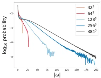
Figure 8 shows the probability distribution function of absolute vorticity in MPIC. The amount of vorticity in the simulation increases rapidly with resolution, consistent with our previous analysis of the root-mean-square vorticity. The amount of vorticity and therefore the stretching rate is very sensitive to resolution. This explains why the mixing rate is also sensitive to resolution.
3.4
Measures of the representation of
small-scale motions
A further measure of the representation of small-scale motions is given by the kinetic energy spectrum(𝑘), which is described in more detail in D18. These are calculated using gridded fields from both models. Results for𝑡 = 6 are shown in Figure 9a,b. The MPIC spectra generally retain more energy at small scales than MONC at the same resolu-tion, but are also characterized by a sharp cut-off, which is due to a spectral filter used to prevent aliasing. We have per-formed sensitivity experiments that show a similar spectrum, but with a longer tail, can be obtained by applying this fil-ter only for vorticity tendencies, and not in the solver (not shown). Both the faster convergence of the rms velocity and the spectra indicate that the velocity field is more detailed in MPIC when the same number of grid points is used, which suggests that small-scale eddies at the cloud edge can be bet-ter resolved. This may seem to contradict the slower reduction in liquid water content in low-resolution MPIC simulations as compared to MONC simulations with the same grid spacing shown in Figure 7. In MPIC, we explicitly represent the dilu-tion process beyond the scale of resolved modilu-tion, whereas in MONC it is handled by the numerics or subgrid parametriza-tion. However, we are currently only representing the effect of resolved dynamics on both entrainment and further mix-ing in MPIC. The mixmix-ing by turbulence on scales that are represented by neither model is therefore underestimated in MPIC.
Implicit MONC simulations also retain more energy on small scales than MONC simulations using the Smagorinsky scheme.
A second measure of small-scale motions can be obtained from the spectrum of the variance of total specific humidity
(𝑘). This is calculated in the same manner as the kinetic energy spectrum. However, to isolate the cloud dynamics from the overall stratification, the mean vertical profile of total humidity has been subtracted before processing the fields.
For MPIC, we use the projection algorithm described in Appendix A to first construct results on a fine grid. Figure 9c shows results for simulations with 643, 1283 and 2563 grid points. Figure 9d shows spectra for the reference simula-tions, which have 10243grid points for MONC and 3843for MPIC.
The humidity spectra of the MPIC simulations again show more variance at the intermediate and small scales, and in this case there is no clear cut-off. Compared to MONC, the MPIC spectra show a slope that is constant over a range that extends out to much smaller scales. This shows how additional detail below the grid scale is captured in MPIC simulations as compared to MONC due to the subgrid parcel representation.
4
T H E O R I G I N O F I N - C L O U D A I R
In this section we illustrate how MPIC can be used to tackle Lagrangian questions which are challenging to address in a Eulerian model. A tracer was added to track the level of origin of parcels. This tracer is treated in the same way as liquid water buoyancy and humidity when splitting and redistribution occurs.1
Figure 10 shows the vertical displacement of parcels from their altitude at𝑡=0 for an MPIC simulation with 2563grid points. This exhibits various noteworthy features. At𝑡=4, a region of in-cloud air originating from lower layers is shown in red between𝑧= 0.5 and𝑧 =0.7. This region has a sharp edge, beyond which there is an environment where subsidence has occurred. The effect of subsidence appears strongest at a level below the rising updraught. The cloud has entrained air at the centre of the updraught, which has ascended less than the air in the vortex ring. A column of rising air is found here, which is consistent with observational and modelling studies of cumulus convection (Blythet al., 2005). The region above the updraught has also ascended.
At𝑡 = 6, there is additional entrainment of air that has come down at the side of the cloud and is rising again. Pockets of this entrained air appear to have mixed into the cloud at𝑡= 8. Though these pockets have descended, they have done so by a relatively small amount, which is consistent with earlier work on convection in moist environments (Blythet al., 1988;
Heuset al., 2008; Böinget al., 2014). At this time, the air
above the updraught has experienced a net descent and gravity waves become evident. A region of net descent appears below the cloud at𝑧∕𝐿𝑧≈0.3. This region separates the cloud from another region of net ascent in the neutally stratified boundary layer below.
5
C O N C L U S I O N S
The development of a warm, moist thermal was simulated in a novel essentially Lagrangian model, MPIC, as well as in the Met Office NERC Cloud model, MONC. The simulation was designed to capture the effects of latent heat release and evaporation, but is not aiming to address a particular type of atmospheric situation.
The overall development of the cloud is in good agree-ment between the MPIC and MONC simulations, as shown both in visual comparisons of the flow structure as well as in quantitative bulk measures of flow properties. The
1For studies that trace the origin of parcels over a longer duration, it could
F I G U R E 9 Kinetic energy spectra at𝑡=6 for (a) simulations with 643(red), 1283(blue) and 2563(black/grey) grid points, and (b) for the
reference simulations with 3843(MPIC) and 10243(MONC) grid points. (c, d) show the corresponding total specific humidity variance spectra.
Here, the MPIC spectra are based on detailed fields derived using the algorithm in Appendix A
F I G U R E 10 Detailed visualization of the vertical displacement of parcels since the beginning of the simulation normalized by the domain height for an MPIC simulation with 2563grid points after (a) 4 , (b) 6 and (c) 8 time units
MPIC simulations capture a large amount of detail in the subgrid-scale flow when compared to MONC at the same grid resolution due to the presence of multiple parcels in each grid box. This has been shown in comparisons of cross-sections and in corresponding spectra across model resolutions.
Subgrid-scale mixing is weaker in all the MPIC sim-ulations than in MONC. Whereas low-resolution MONC simulations tend not to represent the cloud structure as well as low-resolution MPIC simulations, the latter have insufficient
Even the highest resolution MONC and MPIC simulations are not fully in agreement when it comes to the probabil-ity densprobabil-ity function of liquid water. At these resolutions, the MPIC results appear to converge, so this may indicate that the models disagree to some extent. However, the MPIC results also change if they are not calculated on parcels but by projection onto a grid (the projection smooths the field). In this case, they resemble MONC results to a greater extent (Appendix B).
A relatively slow convergence of the properties of the liq-uid water field is not unique to our study. It has also been found in previous work that tried to represent subgrid-scale mixing explicitly, e.g. Jarecka et al. (2009). Apart from this single issue, the models show a remarkable extent of agreement.
When used at sufficiently high resolution, MPIC may provide new perspectives on the role of entrainment and in particular vorticity dynamics in cloud formation (e.g. the role of vorticity extrema in mixing and the presence and dynam-ics of vortex rings). Previous work has shown the usefulness of Lagrangian analysis for understanding cloud processes and turbulence (e.g. Lasher-Trappet al., 2005; Cooperet al., 2013; Böinget al., 2014). MPIC takes this approach a step further by allowing for a Lagrangian analysis which is fully consistent with the model dynamics. A first example of such an analysis was given in Section 4. Further benefits in terms of computa-tional cost can be expected in situations where a large number of tracers is carried by the parcels.
Developing a version of MPIC which uses the same ther-modynamical formulation as the standard version of MONC, and testing this on more representative scenarios driven by surface fluxes, is one of our priorities for further development of MPIC. Furthermore, we want to improve the convergence of the liquid water probability density function with resolution in MPIC. The aim is first to attempt to implement methods that improve resolved and explicitly represented dynamics, for example the use of a finer grid in parts of the dynamical core (in particular for the inversion procedure) and a more phys-ical model of parcel stretch (McKiver and Dritschel, 2003) and splitting. Kaas et al. (2013) also present an approach that looks at explicit deformation of parcels; in terms of mixing, a grid is used here as well, and it shares some prop-erties with the approach currently used in MPIC. A second strategy would be to exploit subgrid information carried by parcels. Particle–particle particle-mesh (PPPM; e.g. Walther and Morgenthal 2002) methods use this strategy, but these are very expensive as many parcel–parcel interactions need to be represented. A stochastic approach based on methods used in dispersion modelling (Thomson, 1987; Weil et al., 2004) could be more suitable, or alternatively a fractal rep-resentation of unresolved turbulence (e.g. Basuet al.2004) could be explored. We believe a mostly parcel-based approach to mixing will be valuable for studies that use Lagrangian
diagnostics. As a last resort, it would be possible to use a gridded approach only to subgrid-scale mixing.
A C K N O W L E D G E M E N T S
The authors gratefully acknowledge support for this research from the EPSRC Maths Foresees Network. The numerical method development was carried out under the grant “A prototype vortex-in-cell algorithm for modelling moist con-vection” from March to October 2016. SJB, DJP and AMB are partially funded through the NERC/Met Office Joint Pro-gramme on Understanding and Representing Atmospheric Convection across Scales (grant NE/N013840/1). DJP is sup-ported by a Royal Society Wolfson Research Merit Award and by the Met Office Academic Partnership. This work used the ARCHER UK National Supercomputing Service (http:// www.archer.ac.uk; accessed 3 April 2019). This research was supported in part by the National Science Foundation under Grant No. NSF PHY17-48958 (in particular, SB benefited from participation in the KITP Program on Planetary Bound-ary Layers in Atmospheres, Oceans, and Ice on Earth and Moons).
R E F E R E N C E S
Abel, S.J. and Shipway, B. (2007) A comparison of cloud-resolving model simulations of trade wind cumulus with aircraft observations taken during RICO.Quarterly Journal of the Royal Meteorological Society, 133, 781–794.
Aranami, K., Davies, T. and Wood, N. (2015) A mass restoration scheme for limited-area models with semi-Lagrangian advection.Quarterly Journal of the Royal Meteorological Society, 141, 1795–1803. Basu, S., Foufoula-Georgiou, E. and Porté-Agel, F. (2004) Synthetic
tur-bulence, fractal interpolation, and large-eddy simulation.Physical Review E, 70, 026310.
Blyth, A.M., Lasher-Trapp, S. and Cooper, W. (2005) A study of ther-mals in cumulus clouds.Quarterly Journal of the Royal Meteorolog-ical Society, 131, 1171–1190.
Blyth, A.M., Cooper, W.A. and Jensen, J.B. (1988) A study of the source of entrained air in Montana cumuli. Journal of the Atmospheric Sciences, 45, 3944–3964.
Böing, S.J., Jonker, H.J., Nawara, W.A. and Siebesma, A.P. (2014) On the deceiving aspects of mixing diagrams of deep cumulus convec-tion.Journal of the Atmospheric Sciences, 71, 56–68.
Brown, N., Weiland, M., Hill, A., Shipway, B., Maynard, C., Allen, T. and Rezny, M. (2015)A highly scalable Met Office NERC Cloud model In: Proceedings of the 3rd International Conference on Exas-cale Applications and Software.pp. 132–137. Edinburgh: University of Edinburgh.
Cooper, W., Lasher-Trapp, S.G. and Blyth, A.M. (2013) The influence of entrainment and mixing on the initial formation of rain in a warm cumulus cloud. Journal of the Atmospheric Sciences, 70, 1727–1743.
conservative dynamical fields. Quarterly Journal of the Royal Meteorological Society, 123, 1097–1130.
Dritschel, D.G., Böing, S.J., Parker, D.J. and Blyth, A.M. (2018) The moist parcel-in-cell method for modelling moist convection. Quar-terly Journal of the Royal Meteorological Society, 144, 1695–1718. Fontane, J. and Dritschel, D.G. (2009) The HyperCASL Algorithm:
a new approach to the numerical simulation of geophysical flows.
Journal of Computational Physics, 228, 6411–6425.
Grabowski, W.W. and Clark, T. (1993) Cloud-environment interface instability: Part II: Extension to three spatial dimensions.Journal of the Atmospheric Sciences, 50, 555–573.
Heus, T., Van Dijk, G., Jonker, H.J. and Van den Akker, H.E. (2008) Mixing in shallow cumulus clouds studied by Lagrangian particle tracking. Journal of the Atmospheric Sciences, 65, 2581–2597.
Hohenegger, C., Schlemmer, L. and Silvers, L. (2015) Coupling of convection and circulation at various resolutions.Tellus A, 67. 26678.
Jarecka, D., Grabowski, W.W. and Pawlowska, H. (2009) Modeling of subgrid-scale mixing in large-eddy simulation of shallow convec-tion.Journal of the Atmospheric Sciences, 66, 2125–2133. Kaas, E. (2008) A simple and efficient locally mass conserving
semi-Lagrangian transport scheme.Tellus A, 60, 305–320. Kaas, E., Sørensen, B., Lauritzen, P.H. and Hansen, A.B. (2013) A
hybrid Eulerian–Lagrangian numerical scheme for solving prognos-tic equations in fluid dynamics.Geoscientific Model Development, 6, 2023–2047.
Langhans, W., Schmidli, J. and Schär, C. (2012) Bulk convergence of cloud-resolving simulations of moist convection over complex terrain.Journal of the Atmospheric Sciences, 69, 2207–2228. Lasher-Trapp, S.G., Cooper, W.A. and Blyth, A.M. (2005) Broadening of
droplet size distributions from entrainment and mixing in a cumulus cloud.Quarterly Journal of the Royal Meteorological Society, 131, 195–220.
Lauritzen, P.H. and Thuburn, J. (2012) Evaluating advection/transport schemes using interrelated tracers, scatter plots and numerical mix-ing diagnostics. Quarterly Journal of the Royal Meteorological Society, 138, 906–918.
Leonard, B., MacVean, M. and Lock, A.P. (1993)Positivity-preserving numerical schemes for multidimensional advection. NASA Lewis Research Center. Tech. Rep.
Mason, P.J. and Brown, A.R. (1999) On subgrid models and filter opera-tions in large eddy simulaopera-tions.Journal of the Atmospheric Sciences, 56, 2101–2114.
Matheou, G. (2011) On the fidelity of large-eddy simulation of shallow precipitating cumulus convection.Monthly Weather Review, 139, 2918–2939.
McKiver, W. and Dritschel, D.G. (2003) The motion of a fluid ellipsoid in a general uniform background flow.Journal of Fluid Mechanics, 474, 147–173.
Ogura, Y. (1963) The evolution of a moist convective element in a shallow, conditionally unstable atmosphere: a numerical calculation.
Journal of the Atmospheric Sciences, 20, 407–424.
Paluch, I.R. (1979) The entrainment mechanism in Colorado cumuli.
Journal of the Atmospheric Sciences, 36, 2467–2478.
Panosetti, D., Böing, S.J., Schlemmer, L. and Schmidli, J. (2016) Ide-alized large-eddy and convection-resolving simulations of moist convection over mountainous terrain.Journal of the Atmospheric Sciences, 73, 4021–4041.
Petch, J.C. and Gray, M.E.B. (2001) Sensitivity studies using a cloud-resolving model simulation of the tropical west Pacific.Quarterly Journal of the Royal Meteorological Society, 127, 2287–2306.
Piacsek, S.A. and Williams, G.P. (1970) Conservation properties of con-vection difference schemes.Journal of Computational Physics, 6, 392–405.
Pincus, R., Barker, H.W. and Morcrette, J.-J. (2003) A fast, flexible, approximate technique for computing radiative transfer in inhomoge-neous cloud fields.Journal of Geophysical Research, Atmospheres, 108(D13). https://doi.org/10.1029/2002JD003322.
Pressel, K., Kaul, C., Schneider, T., Tan, Z. and Mishra, S. (2015) Large-eddy simulation in an anelastic framework with closed water and entropy balances.Journal of Advances in Modeling Earth Sys-tems, 7, 1425–1456.
Siebesma, A.P. and Cuijpers, J. (1995) Evaluation of parametric assump-tions for shallow cumulus convection.Journal of the Atmospheric Sciences, 52, 650–666.
Smagorinsky, J. (1963) General circulation experiments with the prim-itive equations: I. The basic experiment.Monthly Weather Review, 91, 99–164.
Stevens, B., Moeng, C.-H., Ackerman, A.S., Bretherton, C.S., Chlond, A., de Roode, S., Edwards, J., Golaz, J.-C., Jiang, H., Khairout-dinov, M., Kirkpatrick, M.P., Lewellen, D.C., Lock, A.P., Müller, F., Stevens, D.E., Whelan, E. and Zhu, P. (2005) Evaluation of large-eddy simulations via observations of nocturnal marine stra-tocumulus.Monthly Weather Review, 133, 1443–1462.
Stevens, D.E. and Bretherton, C.S. (1999) Effects of resolution on the simulation of stratocumulus entrainment.Quarterly Journal of the Royal Meteorological Society, 125, 425–439.
Thomson, D.J. (1987) Criteria for the selection of stochastic models of particle trajectories in turbulent flows.Journal of Fluid Mechanics, 180, 529–556.
Tsang, Y.-K. and Vallis, G.K. (2018) A stochastic Lagrangian basis for a probabilistic parameterization of moisture condensation in Eulerian models.Journal of Atmospheric Sciences, 75, 3925–3941. Twomey, S. (1966) Computations of rain formation by coalescence.
Journal of the Atmospheric Sciences, 23, 405–411.
Walther, J.H. and Morgenthal, G. (2002) An immersed interface method for the vortex-in-cell algorithm. Journal of Turbulence, 3(N39). https://doi.org/10.1088/1468-5248/3/1/039.
Weil, J.C., Sullivan, P.P. and Moeng, C.-H. (2004) The use of large-eddy simulations in Lagrangian particle dispersion models.Journal of the Atmospheric Sciences, 61, 2877–2887.
Zerroukat, M., Wood, N. and Staniforth, A. (2002) SLICE: a Semi-Lagrangian Inherently Conserving and Efficient scheme for transport problems.Quarterly Journal of the Royal Meteorological Society, 128, 2801–2820.
How to cite this article: Böing SJ, Dritschel DG, Parker DJ, Blyth AM. Comparison of the Moist Parcel-in-Cell (MPIC) model with large-eddy
A P P E N D I C E S
A : A N A L G O R I T H M F O R R E C O N S T R U C T I N G P A R C E L P R O P E R T I E S O N T H E F I N E G R I D
In some of our analysis, parcel properties are interpolated to a grid with a grid spacing that is six times finer than that of the grid used in the vorticity inversion. This approach is useful, for example, for producing two-dimensional cross-sections with a detailed representation of the flow field. While the tri-linear interpolation algorithm used in the vorticity solver aims to find mean parcel properties on a grid (where the spacing is coarser than the parcel radius), the fine grid recon-struction algorithm aims to represent the parcel properties at a scale similar to the smallest parcels. This requires a different approach, because parcel spacing and size vary.
The interpolation algorithm is used to calculate a represen-tative value of a field at a locationx̄in the domain, where the overline denotes interpolated values. As an example, we con-sider the interpolated humidity field ̄𝑞(x̄), which results from taking a weighted sum over the parcels in the domain:
̄𝑞(x̄) =
∑
𝑖∈𝜇(x̄,x𝑖, 𝑉𝑖)𝑞𝑖
∑
𝑖∈𝜇(x̄,x𝑖, 𝑉𝑖) .
(A1)
Here,𝑉𝑖is the parcel volume and𝜇a weighting function. For each parcel, an equivalent radius is defined as
𝑟𝑖=
( 3𝑉𝑖
4𝜋 )1∕3
. (A2)
The weights are chosen to meet following conditions:
1. The weights are isotropic, that is, they depend only on the Euclidean distance𝑟≡‖x̄−x𝑖‖.
2. There is a maximum radius of influence𝑟m, which is the same for each parcel. Outside this radius of influence,
𝜇(x̄,x𝑖, 𝑉𝑖) =0. On the other hand, at each point in space, there must be at least one parcel which contributes tō𝑞(x̄). As each grid box is guaranteed to contain at least one parcel, we can choose
𝑟m= (1+𝜀) √
Δ2
𝑥+ Δ2𝑦+ Δ2𝑧. (A3)
Here,𝜀is a small number (e.g. 0.02; this merely serves to avoid division by small numbers) andΔ𝑥∕𝑦∕𝑧 denotes
the grid spacing of the (vorticity) inversion grid, so that
𝑟mis marginally bigger than the maximum distance within an inversion grid box.
3. The total contribution of a parcel to the three-dimensional projection domain (here the entire domain) is equal to its
volume, that is,
∫ 𝜇(x̄,x𝑖, 𝑉𝑖)d𝑿 =𝑉𝑖. (A4)
This condition holds for parcels for which the projec-tion does not extend beyond the domain top or bottom, otherwise the contribution of a parcel is equal to the con-tribution it gives on the interior of the domain using our method.
4. The contribution of a parcel decreases rapidly when
𝑟 > 𝑟𝑖.
In order to meet these conditions,𝜇(𝑟)is chosen as:
𝜇(𝑟) =𝑉𝑖𝑓(𝑟)∕𝑁. (A5)
Here,𝑓(𝑟)specifies a radial dependence and𝑁is a normal-ization factor, chosen such that
𝑁=
∫ 𝑓(𝑟)d𝑿. (A6)
We employ a Gaussian dependence on radius here:
𝑓(𝑟) =
{
e−(𝑟∕𝑟𝑖)2−e−(𝑟m∕𝑟𝑖)2 𝑟 < 𝑟m,
0 𝑟≥𝑟m. (A7)
This implies
𝑁 =
∫
𝑟m
𝑟=0
4𝜋𝑟2(e−(𝑟∕𝑟𝑖)2−e−(𝑟m∕𝑟𝑖)2)d𝑟
=𝜋𝑟2𝑖
(
𝑟𝑖√𝜋erf(𝑟m∕𝑟𝑖) −2𝑟me(−𝑟
2 m∕𝑟2𝑖)
)
−4𝜋 3 𝑟
3 me−(𝑟m∕𝑟𝑖)
2
. (A8)
Other choices of𝑓(𝑟)can be made for𝑟 < 𝑟mthat also lend themselves to analytical integration; in particular the second power within the exponential function can easily be replaced by the third or fourth power. The choice of function impacts on the character of high-frequency modes in the projected field.
B : R E C O N S T R U C T I N G T H E L I Q U I D W A T E R F I E L D F R O M P A R C E L D A T A
In Section 3.3, we used the parcel properties to derive the statistics of the liquid water field. In practice, we might need to reconstruct the liquid water field on the grid in order to cou-ple the dynamics to other processes (e.g. a radiative transfer scheme).
ql
F I G U R E B1 Liquid water specific humidity pdf at𝑡=6 in the 3843MPIC simulation, as diagnosed using different methods
distribution function from a 5123MONC simulation with the Smagorinsky closure is given as a reference.
a. If only the probability distribution function itself needs to be calculated, this can be done directly from the parcels. However, when the spatial distribution is also important, a different approach is needed.
b. One might simply derive the mean liquid water content of each grid box using the algorithm described in D18. This approach conserves the total liquid water content but has two drawbacks. First of all, some grid boxes are partially cloudy but are now simply seen as containing liquid water, so the cloud fraction increases. In addition, the extremes in the liquid water distribution are no longer present in the gridded field.
c. The detailed projection scheme described in Appendix A can be used. Here, 𝑞 is calculated on the fine grid using the algorithm in the Appendix and 𝑞𝑙 is calcu-lated from the field of 𝑞. This approach is much more computationally costly, but it gives a better probability distribution than the coarse grid approaches and retains small-scale features. This approach is useful mainly for detailed analysis of a limited number of snapshots from MPIC.
d. A fourth approach would be to partition each grid box into a cloudy and a non-cloudy part (as is often done in radiative transfer), and to separately determine the mean value in the cloudy and the non-cloudy parts. This results in the correct cloud fraction and total liquid water content, but both high and low values of liquid water content are under-represented. This is an example of how MPIC’s subgrid-scale information (the cloud frac-tion) can be used. It is possible to extend this, and for example to consider the variance of liquid water within the cloudy part of each grid box, fit an assumed probabil-ity distribution function, and use this in radiative transfer calculations.