pygist pdf

(1)

November 23, 1998

UCRL-MA-128569, Manual 4

The Python Graphics Interface, Part IV

Python Gist Graphics Manual

Written by

(2)

Python Gist Graphics Manual

Copyright (c) 1996.

The Regents of the University of California.

Permission to use, copy, modify, and distribute this software for any purpose without fee is hereby granted, pro-vided that this entire notice is included in all copies of any software which is or includes a copy or modification of this software and in all copies of the supporting documentation for such software.

This work was produced at the University of California, Lawrence Livermore National Laboratory under contract no. W-7405-ENG-48 between the U.S. Department of Energy and The Regents of the University of California for the op-eration of UC LLNL.

DISCLAIMER

(3)

1

Table of Contents

CHAPTER 1:

The Python Graphics Interface

1

Overview of the Python Graphics Interface 1 Using the Python Graphics Interface 2 About This Manual 3

CHAPTER 2:

Introduction to Python Gist Graphics

5

PyGist 2-D Graphics 5 PyGist 3-D Graphics 7

General overview of module pl3d 7 Overview of module plwf 8

Overview of module slice3 9 movie.py: PyGist 3-D Animation 9 Function Summary 12

CHAPTER 3:

Control Functions

17

Device Control 17 Window Control 17

Hard Copy and File Control 19 Other Controls 21

animate: Control Animation Mode 21 palette: Set or Retrieve Palette 21 plsys: Set Coordinate System 22 redraw: Redraw X window 22

CHAPTER 4:

Plot Limits and Scaling

23

Setting Plot Limits 23

limits: Save or Restore Plot Limits 23 ylimits: Set y-axis Limits 24

Scaling and Grid Lines 24

logxy: Set Linear/Log Axis Scaling 24 gridxy: Specify Grid Lines 25

Zooming Operations 25

CHAPTER 5:

Two-Dimensional Plotting Functions

27

(4)

plmesh: Set Default Mesh 29 plm: Plot a Mesh 30

plc: Plot Contours 32 plv: Plot a Vector Field 33 plf: Plot a Filled Mesh 35 plfc: Plot filled contours 37

plfp: Plot a List of Filled Polygons 39 pli: Plot a Cell Array 40

pldj: Plot Disjoint Lines 42 plt: Plot Text 43

pltitle: Plot a Title 44 Plot Function Keywords 45

CHAPTER 6:

Inquiry and Miscellaneous Functions

49

Inquiry and Editing Functions 49 plq: Query Plot Element Status 49 pledit: Change Plotting Properties 49 pldefault: Set Default Values 50 Miscellaneous Functions 52 bytscl: Convert to Color Array 52

histeq_scale: Histogram Equalized Scaling 52 mesh_loc: Get Mesh Location 52

mouse: Handle Mouse Click 53 moush: Mouse in a Mesh 54 pause: Pause 54

CHAPTER 7:

Three-Dimensional Plotting Functions

55

Setting Up For 3-D Graphics 55 The Plotting List 55

Functions For Setting Viewing Parameters 56 Lighting Parameters 57

Display List 58

3-D Graphics Control Functions 58 Getting a Window 58

Displaying the Gnomon 58 Plotting the Display List 59

The variable _draw3 and the idler 60 Data Setup Functions for Plotting 61 Creating a Plane 61

Creating a mesh3 argument 61 The Slicing Functions 64

slice3mesh: Pseudo-slice for a surface 64

(5)

3

slice2 and slice2x: Slicing Surfaces with planes 66 At Last - the 3-D Plotting Functions 67

plwf: plot a wire frame 67 pl3surf: plot a 3-D surface 71

pl3tree: add a surface to a plotting tree 74

Contour Plotting on Surfaces: plzcont and pl4cont 77 Animation: movie and spin3 80

The movie module and function 80 The spin3 function 83

Syntactic Sugar: Some Helpful Functions 85 Specifying the palette to be split: split_palette 85

Saving and restoring the view and lighting: save3, restore3 85

CHAPTER 8:

Useful Functions for Developers

87

Find 3D Lighting: get3_light 87

Get Normals to Polygon Set: get3_normal 87 Get Centroids of Polygon Set: get3_centroid 88 Get Viewer’s Coordinates: get3_xy 88

Add object to drawing list: set3_object 88 Sort z Coordinates: sort3d 89

Set the cmax parameter: lightwf 89

Return a Wire Frame Specification: xyz_wf 90 Calculate Chunks of Mesh: iterator3 90

Get Vertex Values of Function: getv3 91 Get Cell Values of Function: getc3 92

Controlling Points Close to the Slicing Plane: _slice2_precision 92 Scale variables to a palette: bytscl, split_bytscl 93

Return Vertex Coordinates for a Chunk: xyz3 93 Find Corner Indices of List of Cells: to_corners3 94 Timing: timer, timer_print 94

CHAPTER 9:

Maintenance: Things You Really Didn’t Want to Know

95

The Workhorse: gistCmodule 95 Memory Maintenance: PyObjects 95 Memory Management: ArrayObjects 97 Memory Management: naked memory 98 Computing contour curves: contour 98

Computing slices: slice2, slice2x, _slice2_part 99 Some Yorick-like Functions: yorick.py 101 Additional Array Operations: arrayfnsmodule 102 Counting Occurrences of a Value: histogram 102

(6)

Interpolating Values: interp 103 Digitizing an array: digitize 104

Reversing a Two-Dimensional array: reverse 104 Obtaining an Equally-Spaced Array of Floats: span 104 Effective Length of an Array: nz 105

Finding Edges Cut by Isosurfaces: find_mask 105 Order Cut Edges of a cell: construct3 105

Expand cell-centered values to node-centered values: to_corners 106 More slice3 details 107

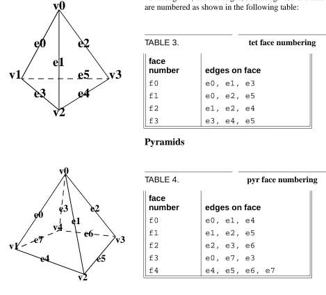
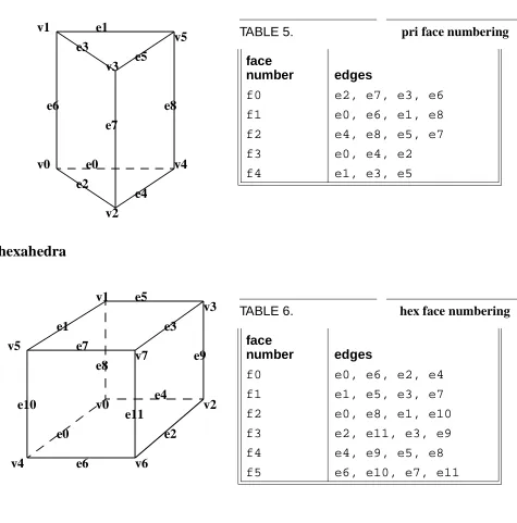
Standard ordering for the four types of mesh cells 107

(7)

(8)

(9)

November 23, 1998

UCRL-MA-128569, Manual 4

C H A P T E R 1 :

The Python Graphics

Interface

1.1

Overview of the Python Graphics Interface

The Python Graphics Interface (abbreviated PyGraph) provides Python users with capabilities for plotting curves, meshes, surfaces, cell arrays, vector fields, and isosurface and plane cross sections of three dimensional meshes, with many options regarding line widths and styles, markings and labels, shading, contours, filled contours, coloring, etc. Animation, moving light sources, real-time rotation, etc., are also available. PyGraph is intended to supply a choice of easy-to-use interfaces to graphics which are relatively independent of the underlying graphics engine, concealing the technical details from all but the most intrepid users. Obviously different graphics engines offer different features, but the intention is that when a user requests a particular type of plot which is not available on a particular engine, the low level interface will make an intelligent guess and give some approximation of what was asked for.

There are two such graphics packages which are relatively independent of the underlying plotting library. The Object-Oriented Graphics (OOG) Package defines geometric objects (Curves, Surfaces, Meshes, etc.), Graph objects which can be given one or more geometric objects to plot, and Plotter ob-jects, which receive geometric objects to plot from Graph obob-jects, and which interface with the graph-ics engine(s) to do the actual plotting. A Graph can create its own Plotter, or the more capable user can create one or more, handy when one wishes (for instance) to plot on a remote machine, or to open graphics windows of different types at the same time. The second such package is called EZPLOT; it is built on top of OOG, and provides an interface similar to the command-line interface of the Basis EZN package. Some of our long-time users may be more comfortable with this package, until they have mastered the concepts of object-oriented design.

As mentioned above, a Graph object needs at least one Plotter object to plot itself; only the Plotter objects need know about graphics engines. At present we have two types of Plotter objects, one which knows about Gist and one which knows about Narcisse. Some power users may prefer to use the lower-level library-specific function calls, but most users will use EZPLOT or OOG.

(10)

anima-CHAPTER 1: The Python Graphics Interface

tion (moving light sources and rotations). The Python Gist module gist.py and the associated Py-thon extension gistCmodule provide a Python interface to this library (referred to as PyGist).

Narcisse is a graphics library developed at out sister laboratory at Limeil in France. It is especially strong in high-quality 3-D surface rendering. Surfaces can be colored in a variety of ways, including colored wire mesh, colored contours, filled contours, and colored surface cells. Some combinations of these are also possible. We have also added the capability of doing isosurfaces and plane sections of meshes, which is not available in the original Narcisse. The Python Narcisse module narcissemod-ule (referred to as PyNarcisse) provides a low-level Python interface to this library. Unlike Gist, Nar-cisse does not currently write automatically to standard files such as PostScript or CGM, although it writes profusely to its own type of files unless inhibited from doing so, as described below. However, there is a "Print" button in the Narcisse graphics window, which opens a dialog that allows you to write the current plot to a postscript file or to send it to a postscript printer.

1.2

Using the Python Graphics Interface

In order to use PyGraph, you first need to have Python installed on your system. If you do not have Python, you can obtain it free from the Python pages at http://www.python.org. You may need the help of your system administrator to install it on your machine. Once you have Python, you have to know at least a smattering of the language. The best way to do this is to download the excel-lent tutorial from the Python pages, sit down at your computer or terminal, and work your way through it.

Before using the Python Graphics Interface, you should set some environment variables as follows.

• Your PATH variable should contain the path to the python executable.

• You should set a PYTHONPATH variable to point to all directories that contain Python exten-sions or modules that you will be loading, which may include the OOG modules, ezplot, and

narcissemodule or gistCmodule. Check with your System Manager for the exact speci-fications on your local systems.

• Unless you create your own plotter objects, PyGraph will create a default Gist Plotter which will plot to a Gist window only. If you want your default Plotter to be a Narcisse Plotter, then set the variable PYGRAPH to Nar or Narcisse.

A Gist Plotter object automatically creates its own Gist window and then plots to that window. Nar-cisse, however, works differently. Narcisse is established as a separately running process, to which the Plotter communicates via sockets. Thus, to run a Narcisse Plotter, you must first open a Narcisse.1 To do so, you need to go through the following steps:

1. Set your environment variable PORT_SERVEUR2 to 0.

(11)

3

About This Manual

2. Start up Narcisse by typing in the command Narcisse &. It will take a few moments for the Narcisse GUI to open, then immediately afterwards it will be covered by an annoying window which you can eliminate by clicking its OK button.

3. You will note that there is a server port number given on the GUI. Set your PORT_SERVEUR vari-able to this value.

4. Narcisse has an annoying habit of saving everything it does to a multitude of files, and notifying you on the fly of all its computations. If you do a lot of graphics, these files can quickly fill up your quota. In addition, the running commentary on file writing and computation on the GUI is time-consuming and slows Narcisse down to a truly glacial pace. To avoid this, you need to turn off a number of options via the GUI before you begin. They are all under the STATE submenu of the

FILE menu, and should be set as follows: set ‘‘Socket compute’’ to ‘‘no,’’ set ‘‘File save’’ to ‘‘nothing,’’ set ‘‘Config save’’ to ‘‘no,’’ and set ‘‘Ihm compute’’ to ‘‘no.’’ (‘‘IHM’’ are the French initials for ‘‘GUI.’’)

1.3

About This Manual

This manual is part of a series of manuals documenting the Python Graphics Interface (PyGraph). They are:

• I. EZPLOT User Manual

• II. Object-Oriented Graphics Manual

• III. Plotter Objects Manual

• IV. Python Gist Graphics Manual

• V. Python Narcisse Graphics Manual

EZPLOT is a command-line oriented interface that is very similar to the EZN graphics package in Basis. The Object-Oriented Graphics Manual provides a higher-level interface to PyGraph. The re-maining manuals give low-level plotting details that should be of interest only to computer scientists developing new user-level plot commands, or to power users desiring more precise control over their graphics or wanting to do exotic things such as opening a graphics window on a remote machine.

PyGraph is available on Sun (both SunOS and Solaris), Hewlett-Packard, DEC, SGI workstations, and some other platforms. Currently at LLNL, Narcisse is installed only on the X Division HP and So-laris boxes, however, and Narcisse is not available for distribution outside this laboratory. Our French colleagues are going through the necessary procedures for public release, but these have not yet been crowned with success. Gist, however, is publicly available as part of the Yorick release, and may be obtained by anonymous ftp from ftp-icf.llnl.gov; look in the subdirectory /ftp/pub/ Yorick.

A great many people have helped create PyGraph and its documentation. These include

(12)

CHAPTER 1: The Python Graphics Interface

• Zane Motteler of LLNL, who wrote narcissemodule, ezplot, the OOG, and some other auxiliary routines, and who wrote much of the documentation, at least the part that was not bla-tantly stolen from David Munro and Steve Langer (see below);

• Paul Dubois of LLNL, who wrote the PDB and Ranf modules, and who worked with Konrad Hinsen (Laboratoire de Dynamique Moleculaire, Institut de Biologie Structurale, Grenoble, France) and James Hugunin (Massachusetts Institute of Technology) on NumPy, the numeric ex-tension to Python, without which this work could not have been done;

• Fred Fritsch of LLNL, who produced the templates and did some of the writing of this documen-tation;

• Our French collaborators at the Centre D’Etudes de Limeil-Valenton (CEL-V), Commissariat A L’Energie Atomique, Villeneuve-St-Georges, France, among whom are Didier Courtaud, Jean-Philippe Nomine, Pierre Brochard, Jean-Bernard Weill, and others;

• David Munro of LLNL, the man behind Yorick and Gist, and Steve Langer of LLNL, who col-laborated with him on the 3-D interpreted graphics in Yorick. We have also shamelessly stolen from their Gist documentation; however, any inaccuracies which crept in during the transmission remain the authors’ responsibility.

The authors of this manual stand as representative of their efforts and those of a much larger num-ber of minor contributors.

(13)

November 23, 1998

UCRL-MA-128569, Manual 4

C H A P T E R 2 :

Introduction to

Python Gist Graphics

Gist is a scientific graphics library written in C by David H. Munro of Lawrence Livermore National Laboratory. It features support for three common graphics output devices: X-Windows, (color) Post-script, and ANSI/ISO Standard Computer Graphics Metafiles (CGM). The library is small (written directly to Xlib), portable, efficient, and full-featured. It produces x-vs-y plots with ‘‘good’’ tick marks and tick labels, 2-D quadrilateral mesh plots with contours, filled contours, vector fields, or pseudocolor maps on such meshes. Some 3-D plot capabilities are also available. The Python Gist module gist.py and the Python extension gistCmodule provide a low-level Python interface to this library as far as 2-D is concerned. In addition, there are several other Python modules which interface with the 2-D graphics to produce 3-D graphics and animation: movie.py (supporting ani-mation), pl3d.py (basic 3-D plotting algorithms), plwf.py (wire frame plotting), and

slice3.py (providing mesh capability with isosurface and plane slicing). Collectively all of these interface modules are known as PyGist.

This chapter will summarize the plotting features that are available in PyGist, and list (in the final section) the functions that are to be described in future chapters.

2.1

PyGist 2-D Graphics

In two dimensions, PyGist supplies functions to plot curves, meshes (with various combinations of contours, filled mesh cells, and vector fields on the mesh, with color-filled contours in the future), sets of filled polygons, cell arrays, sets of disjoint lines, text strings, and a title. These are all provided by the Python module gist.py.

We will show a couple of simple examples below to give the reader a flavor of the interface.

Example 1

In the first example we simply plot a straight line from (1,0) to (2,1). Note that only two coor-dinates are specified for y; x is not specified. In such a case, the values of x default to the integers from 1 to len (y).

from gist import * # Put plot functions in name space.

pldefault (marks = 1, width = 0, type = 1, style = "work.gs", dpi = 100) # Set some defaults.

(14)

CHAPTER 2: Introduction to Python Gist Graphics

plg ( [0, 1]) # The first positional argument is y.

As can be deduced from this example, most PyGist function calls can be augmented with a number of optional keyword arguments. These can (usually) be supplied in any order, and each is of the form

keyword=value. Throughout this manual, a list of the available keywords for a function is given with the description of the function.

Example 2

The next example computes and plots a set of nested cardioids in the primary and secondary colors.

fma()

x = 2 * pi * arange (200, typecode = Float) / 199.0 for i in range (1, 7):

r = 0.5 * i - (5 - 0.5 * i) * cos (x)

s = 'curve ' + `i` #Backticks produce something printable. plg (r * sin (x), r * cos (x), marks = 0, color = - 4 - i, legend = s) # Curves unmarked, in colors.

(15)

7

PyGist 3-D Graphics

2.2

PyGist 3-D Graphics

2.2.1

General overview of module

pl3d

The Python module pl3d.py contains the basic 3-D plotting algorithms and is the workhorse of the PyGist 3-D graphics. The philosophy behind 3-D plotting is to instruct the 3-D plotting functions to accumulate information about the plot until such time as the information is complete, and then ask that the picture be drawn. The information about the plot is stored in a Python list containing the fol-lowing information:

• The orientation of the axes, the location of the origin, and the distance of the viewpoint;

• A set of pairs of plot functions to call and their argument lists; and

• A collection of one or more quintuples specifying the lighting (it is possible to specify multiple light sources).

The first and third items above default to reasonable values if the user does not call functions (e. g.,

rot3, mov3, aim3, set3_light., etc.) to set them. The list described in the second bullet is built by a set of one or more calls to the various plotting functions, which create the list of arguments for each call and then add the function name and argument list pair to the plot list for future execution. When the list is complete, a call to draw3 causes the list to be traversed, and at this point each plot-ting function on the list executes with the argument list that was built when it was first called.

2.2.2

Overview of module

plwf

(16)

deter-CHAPTER 2: Introduction to Python Gist Graphics

mined by a simple ‘‘painter’s algorithm’’, which works fairly well if the mesh is reasonably nearly rectilinear, but can fail even then if the viewpoint is chosen to produce extreme fisheye perspective effects. One must look at the resulting plot carefully to be sure the algorithm has correctly rendered the model in each case.

A 3-D wire mesh can also be plotted using shading and lighting effects as determined by values set in the pl3d module; or the zones can be colored (using the current palette) by their average height or by the values of some function, which may be zone-centered or node-centered.

Examples

The following is a fairly simple example of a wire mesh plot.

from pl3d import * set_draw3_ (0)

x = span (-1, 1, 64, 64) y = transpose (x)

z = (x + y) * exp (-6.*(x*x+y*y)) orient3 ( )

light3 ( )

from plwf import * plwf (z, y, x)

[xmin, xmax, ymin, ymax] = draw3(1) limits (xmin, xmax, ymin, ymax)

(17)

9

movie.py: PyGist 3-D Animation

draw3 call then causes the drawing list to be plotted. draw3 returns the maxima and minima of the x and y variables, which must then be sent to the limits function to prevent the plot appearing dis-torted. (Ah, the perils of using low level graphics.)

2.2.3

Overview of module

slice3

Module slice3.py contains two plotting functions of interest. First, pl3surf can be used for graphing surfaces on an arbitrary two-dimensional mesh with filled cells and no mesh lines. (Cur-rently plwf can be used to do the same thing in the case of a mesh all of whose cells are quadrilat-eral, and has more flexibility, in that it allows mesh lines to be drawn and/or allows for the mesh to be see-through.) Secondly, pl3tree is a plotting function that can be called multiple times in order to have several surfaces drawn on the same graph. pl3tree (as its name suggests) creates a tree of val-ues sorted as to when they will be plotted on the screen; if the algorithm works correctly, then more distant cells are plotted first, then covered by closer cells which are plotted later, giving the surface the correct appearance.

Surfaces to be plotted by pl3surf or pl3tree can be generated by taking plane sections of an arbitrary mesh or by creating isosurfaces for some function or functions defined on the mesh. These planes and isosurfaces can themselves be sliced and portions discarded, to enhance visibility of the in-terior. The functions mesh3 and slice3mesh take raw input data and put it into the form accepted by slice3, which can form plane sections or isosurfaces through the mesh. Functions slice2

(which returns the portion of a surface in front of the slicing plane) and slice2x (which returns the two parts of a surface sliced by a plane) complete the triumvirate of slicing functions.

The algorithms in slice3 are independent of the underlying graphics. Thus slice3 may equal-ly well be used with Narcisse graphics.

2.3

movie.py

: PyGist 3-D Animation

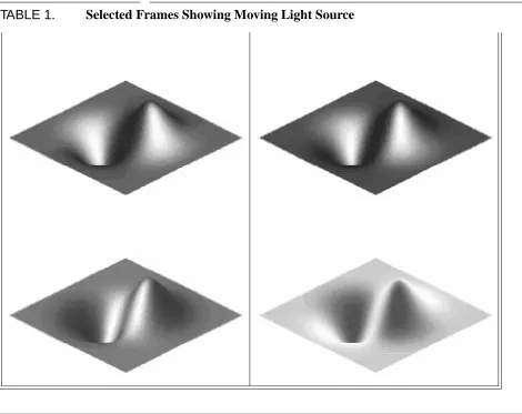
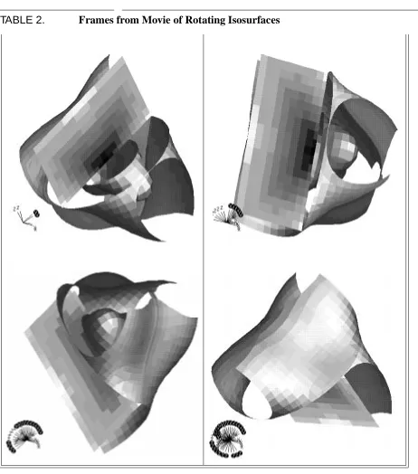
The module movie.py supports 3-D real time animation. Function movie accepts as argument the name of a drawing function which has as its single argument a frame number; movie then calls this drawing function within a loop, halting when the function returns zero. The idea is that the drawing function increments from the previous frame and draws the new frame, returning zero when some pre-defined event takes place, e. g., some set number of frames has been drawn, or a certain amount of time has elapsed. The function spin3 in module pl3d calls movie; the drawing function _spin3 draws the successive frames of a rotating 3-D plot. The demonstration module demo5.py contains an ex-ample of a shaded surface with a moving light source; the drawing function, demo5_light, moves the light and draws the next frame.

Examples

The following example is explained by comments in the code. It is taken from demo5.py. (To repeat, demo5_light is a function which appears in demo5.py.)

(18)

xyz = zeros ( (3, nx, ny, nz), Float)

xyz [0] = multiply.outer ( span (-1, 1, nx), ones ( (ny, nz), Float))

xyz [1] = multiply.outer ( ones (nx, Float),

multiply.outer ( span (-1, 1, ny), ones (nz, Float))) xyz [2] = multiply.outer ( ones ( (nx, ny), Float),

span (-1, 1, nz))

r = sqrt (xyz [0] ** 2 + xyz [1] **2 + xyz [2] **2) theta = arccos (xyz [2] / r)

phi = arctan2 (xyz [1] , xyz [0] + logical_not (r)) y32 = sin (theta) ** 2 * cos (theta) * cos (2 * phi) # mesh3 creates an object which slice3 can slice. The # isosurfaces will be with respect to constant values # of the function r * (1. + y32)].

m3 = mesh3 (xyz, funcs = [r * (1. + y32)])

[nv, xyzv, dum] = slice3 (m3, 1, None, None, value = .50) # (inner isosurface)

[nw, xyzw, dum] = slice3 (m3, 1, None, None, value = 1.) # (outer isosurface)

pxy = plane3 ( array ([0, 0, 1], Float ), zeros (3, Float)) pyz = plane3 ( array ([1, 0, 0], Float ), zeros (3, Float)) [np, xyzp, vp] = slice3 (m3, pyz, None, None, 1)

# (pseudo-colored plane slice)

[np, xyzp, vp] = slice2 (pxy, np, xyzp, vp) # (cut slice in half, discard "back" part) [nv, xyzv, d1, nvb, xyzvb, d2] = \

slice2x (pxy, nv, xyzv, None) # halve inner isosurface [nv, xyzv, d1] = \

slice2 (- pyz, nv, xyzv, None)

# (...halve one of those halves) [nw, xyzw, d1, nwb, xyzwb, d2] = \

slice2x ( pxy , nw, xyzw, None)

# (split outer isosurface in halves) [nw, xyzw, d1] = \

slice2 (- pyz, nw, xyzw, None) # discard half of one half fma () # frame advance

# split_palette causes isosurfaces to be shaded in grey # scale, plane sections to be colored by function values split_palette ("earth.gp")

gnomon (1) # show small set of axes clear3 () # clears drawing list

(19)

11

movie.py: PyGist 3-D Animation

pl3tree (nwb, xyzwb) pl3tree (nv, xyzv) pl3tree (nw, xyzw) orient3 ()

# set lighting parameters for isosurfaces light3 (diffuse = .2, specular = 1)

limits (square=1)

demo5_light (1) # Causes drawing to appear

(20)

2.4

Function Summary

Here is a summary of the functions which are described in the remainder of this manual.

• Control functions (CHAPTER 3: “Control Functions”)

window ( [n] [, <keylist>]) # open or select device n

keywords: display, dpi, dump, hcp, legends, private, style, wait

winkill ( [n]) # delete device n

n = current_window () # determine active device fma () # frame advance

• Plot limits and scaling (CHAPTER 4: “Plot Limits and Scaling”)

old_limits = limits ()

old_limits = limits (xmin [, xmax[, ymin[, ymax]]] [, <keylist>] )

keywords: square, nice, restrict limits (old_limits )

ylimits (ymin[, ymax] ) logxy (xflag[, yflag] ) gridxy (flag )

gridxy (xflag, yflag ) zoom_factor (factor ) unzoom ()

• Two-dimensional plotting functions (CHAPTER 5: “Two-Dimensional Plotting Functions”)

plg (y [, x][, <keylist>] ) # plot a graph

keywords: legend, hide, type, width, color, closed, smooth, marks, marker, mspace, mphase, rays plmesh ([y, x][, ireg][, triangle=tri_array] )

# set default mesh plmesh () # delete default mesh plm ([y, x][, ireg][, <keylist>] )

# plot mesh

keywords: boundary, inhibit, legend, hide, type, width, color, region

plc (z[, y, x][, ireg][, <keylist>] )

# plot contours

keywords: levs, triangle, legend, hide, type, width, color, smooth, marks, marker, mspace, mphase, region

plfc (z[, y, x][, ireg][, <keylist>] )

(21)

13

Function Summary

plv (vy, vx[, y, x][, ireg][, <keylist>] )

# plot vector field

keywords: scale, hollow, aspect, legend, hide, type, width, color, smooth, marks, marker, mspace, mphase, triangle, region

plf (z[, y, x][, ireg][, <keylist>] )

# Plot a filled mesh

keywords: edges, ecolor, ewidth, legend, hide, region, top, cmin, cmax

plfp (z, y, x, n[, <keylist>] )

# Plot filled polygons

keywords: legend, hide, top, cmin, cmax pli (z[[, x0, y0], x1, y1][, <keylist>] )

# Plot a cell array

keywords: legend, hide, top, cmin, cmax pldj (x0, y0, x1, y1[, <keylist>] )

# Plot disjoint lines

keywords: legend, hide, type, width, color plt (text, x, y[, <keylist>] )

keywords: tosys, font, height, opaque, path, justify, legend, hide, color

pltitle (title ) # Plot a title

• Inquiry and Miscellaneous functions (CHAPTER 6: “Inquiry and Miscellaneous Functions”)

plq () # Query plot element status legend_list = plq ()

**** RETURN VALUE NOT YET IMPLEMENTED **** plq (n_element[, n_contour] )

properties = plq (n_element[, n_contour]) pledit ([n_element[, n_contour],] <keylist> )

# Change Plotting Properties of Current Element

The keywords can be any of the keywords that apply to the current element.

pldefault (key1=value1, key2=value2, ... ) # Set default values

The keywords can be most of the keywords that can be passed to the plotting commands.

bytscl (z[, top=max_byte][, cmin=lower_cutoff] [, cmax=upper_cutoff])

# Convert data to color array

histeq_scale (z[, top=top_value][, cmin=cmin][, cmax=cmax]) **** NOT YET IMPLEMENTED **** # Histogram Equalized Scaling

(22)

# Handle Mouse Click moush ([y, x[, ireg]] )

# Return zone index of point clicked in mesh pause (milliseconds) # self-explanatory

• Three-dimensional plotting functions (CHAPTER 7: “Three-Dimensional Plotting Functions”)

orient3 (phi = angle₁, theta = angle₂)

rot3 (xa = angle_x, ya = angle_y, za = angle_z) mov3 (xa = val₁, ya = val₂, za = val₃)

aim3 (xa = val₁, ya = val₂, za = val₃) light3 (ambient=a_level, diffuse=d_level,

specular=s_level, spower=n, sdir=xyz) clear3 ( )

window3 ( [n] [, dump = val] [, hcp = filename]) gnomon ( [onoff] [, chr = <labels>] )

set_default_gnomon ( [onoff])

[lims = ] draw3 ( [called_as_idler = <val>]) limits (lims [0], lims [1], lims [2], lims [3]) set_draw3 (n)

n = get_draw3 ( ) clear_idler ( )

set_idler (func_name) set_default_idler ( ) call_idler ( )

plane3 (<normal>, <point>) mesh3 (x, y, z)

mesh3 (x, y, z, funcs = [f1, f2, ...], [verts = <spec>]) mesh3 (xyz, funcs = [f1, f2, ...])

mesh3 (nxnynz, dxdydz, x0y0z0, funcs = [f1, f2, ...]) slice3mesh (z [, color])

slice3mesh (nxny, dxdy, x0y0, z [, color]) slice3mesh (x, y, z [, color])

slice3 (m3, fslice, nv, xyzv [, fcolor [, flg₁]] [, value = <val>] [, node = flg₂])

[nverts, xyzverts, values] = slice2 (plane, nv, xyzv, vals) [nverts, xyzverts, values, nvertb, xyzvertb, valueb] =

slice2x (plane, nv, xyzv, vals) plwf (z [, y, x] [, <keylist>] )

keywords: fill, shade, edges, ecolor, ewidth, cull, scale, cmax

pl3surf (nverts, xyzverts [, values] [, <keylist>])

(23)

15

Function Summary

pl3tree (nverts, xyzverts [, values] [, <keylist>])

keywords: plane, cmin, cmax, split

• Animation functions (7.7 “Animation: movie and spin3”)

movie (draw_frame [, time_limit = 120.] [, min_interframe = 0.0]

[, bracket_time = array ([2., 2.], Float )] [, lims = None]

[, timing = 0]) spin3 (nframes = 30,

axis = array ([-1, 1, 0], Float), tlimit = 60.,

dtmin = 0.0,

bracket_time = array ([2., 2.], Float), lims = None,

timing = 0,

angle = 2. * pi)

• Syntactic Sugar (7.8 “Syntactic Sugar: Some Helpful Functions”)

split_palette ( [palette_name]) view = save3 ()

(24)

(25)

November 23, 1998

UCRL-MA-128569, Manual 4

C H A P T E R 3 :

Control Functions

This chapter contains all the information you need to control PyGist devices. Device refers to an X window or a hard copy file. In addition, we describe functions which control some aspects of the appearance of the graph.

3.1

Device Control

3.1.1

Window Control

Calling Sequences

window ( [n] [, <keylist>]) winkill ( [n])

n = current_window () fma()

Description

The window function selects device n as the current graphics device. n may range from 0 to 7, inclu-sive. Each graphics device corresponds to an X window, a hardcopy file, or both, depending on the values of the keyword arguments described below. If n is omitted, it defaults to the current active device, if any. window returns the number of the currently active device. winkill deletes the cur-rent graphics device, or device n if n is specified. current_window returns the number of the cur-rent active device, or -1 if there is none. fma frame advances the current graphics device. The current picture remains displayed in the associated X window (if any) until the next element is actu-ally plotted. An fma must be given after the last plot to a hardcopy file for that plot to appear when the file is printed.

The keywords accepted by the window function are

display, dpi, dump, hcp, legends, private, style, wait

and are described in the next subsection.

Keyword Arguments

The following keyword arguments can be specified with this function.

display

(26)

CHAPTER 3: Control Functions

appear (for example, "icf.llnl.gov:0.0"). If not specified, uses your default display (which it gets from your DISPLAY environment variable). Use display = "" (the null string) to create a graphics device which has no associated X window. (You should do this if you want to make plots in a non-interactive batch mode.)

dpi

The allowed values for dpi are 75 and 100. The X window will appear on your default dis-play at 75 dpi, unless you specify the display and/or dpi keywords. A dpi=100 X win-dow is larger than a dpi=75 X window; both represent the same thing on paper.

dump

The dump keyword, if present, controls whether all colors are converted to a gray scale (dump =0, the default), or the current palette is dumped at the beginning of each page of hardcopy output. Set dump to 1 if you are doing color plots. The dump keyword applies only to the spe-cific hardcopy file defined using the hcp keyword (see below) -- use the dump keyword in the

hcp_file command to get the same effect in the default hardcopy file.

hcp

The value of this keyword is a quoted string giving a file name. By default, a graphics window does NOT have a hardcopy file of its own -- any requests for hardcopy are directed to the default hardcopy file, so hardcopy output from any window goes to a single file. By specify-ing the hcp keyword, however, a hardcopy file unique to this window will be created. If the

hcp filename ends in ‘‘.ps’’, then the hardcopy file will be a PostScript file; otherwise, hard-copy files are in binary CGM format. Use hcp ="" (the null string) to revert to the default hardcopy file (closing the window specific file, if any).

In the next section of this manual we shall consider the hardcopy and file functions. Note that the PyGist default is to write to a hardcopy file only on demand. (See function hcp, page 20.)

legends

The legends keyword, if present, controls whether the curve legends are (legends= 1, the default) or are not (legends=0) dumped to the hardcopy file. The legends keyword applies to all pictures dumped to hardcopy from this graphics window. Legends are never plot-ted to the X window.

private

By default, an X window will attempt to use shared colors, which permits several PyGist graphics windows (including windows from multiple instances of Python) to use a common palette. You can force an X window to post its own colormap (set its colormap attribute) with the private=1 keyword. You will most likely have to fiddle with your window manager to understand how it handles colormap focus if you do this. Use private = 0 to return to shared colors.

style

(27)

19

Device Control

dinate systems, tick and label styles, and the like. Here are brief descriptions of the available stylesheets:

axes.gs: axes with labeled tick marks along bottom and left of graph.

boxed.gs: lines all the way around the plot with tick marks, labeled along bottom and left.

boxed2.gs: same as boxed.gs but no tick marks on the top and right sides.

l_nobox.gs: no box, axes, or ticks; graph extends all the way to edge of window.

nobox.gs: indistinguishable from l_nobox.gs.

vg.gs: large tick marks all the way around the graph, but no lines, with large in-frequent labels on the bottom and left.

vgbox.gs: same as vg.gs except with lines all the way around as well

work.gs: small tick marks with small, frequent labels on bottom and left, no lines.

work2.gs: similar to work.gs, but no ticks along top and right.

wait

By default, Python will not wait for the X window to become visible. Code which creates a new window, then plots a series of frames to that window should use wait=1 to assure that all frames are actually plotted.

Examples

The first example ensures that an old window 0 is not hanging around, and then creates a new 100 dpi window.

winkill(0)

window (0, wait = 1, dpi = 100)

The second example changes the style sheet of window 2.

window (2, style = "vgbox.gs")

3.1.2

Hard Copy and File Control

Calling Sequences

eps (name) hcp ()

hcp_file ( [filename] [, dump = 0/1]) filename = hcp_finish ( [n])

hcp_out ( [n] [, keep = 0/1]) hcpon ()

(28)

Descriptions

eps (name)

Write the picture in the current graphics window to the Encapsulated PostScript file name+ ".epsi" (i.e., the suffix .epsi is added to name). The eps function requires the

ps2epsi utility which comes with the project GNU Ghostscript program. Any hardcopy file associated with the current window is first closed, but the default hardcopy file is unaffected. As a side effect, legends are turned off and color table dumping is turned on for the current window. The environment variable PS2EPSI_FORMAT contains the format for the command to start the ps2epsi program.

hcp ()

The hcp function sends the picture displayed in the current graphics window to the hardcopy file. (The name of the default hardcopy file can be specified using hcp_file; each individ-ual graphics window may have its own hardcopy file as specified by the window function.)

hcp_file ( [filename] [, dump = 0/1])

Sets the default hardcopy file to filename. If filename ends with ‘‘.ps’’, the file will be a PostScript file, otherwise it will be a binary CGM file. By default, the hardcopy file name will be ‘‘Aa00.cgm’’, or ‘‘Ab00.cgm’’ if that exists, or ‘‘Ac00.cgm’’ if both exist, and so on. The default hardcopy file gets hardcopy from all graphics windows which do not have their own specific hardcopy file (see the window function). If the dump keyword is present and non-zero, then the current palette will be dumped at the beginning of each frame of the default hardcopy file. This is what you want to do when you want color plots. With dump=0, the default behavior of converting all colors to a gray scale is restored.

filename = hcp_finish ( [n])

Close the current hardcopy file and return the filename. If n is specified, close the hcp file associated with window n and return its name; use hcp_finish(-1) to close the default hardcopy file.

hcp_out ( [n] [, keep = 0/1])

NOT YET IMPLEMENTED

Finishes the current hardcopy file and sends it to the printer. If n is specified, prints the hcp

file associated with window n; use hcp_out(-1) to print the default hardcopy file. Unless the keep keyword is supplied and non-zero, the file will be deleted after it is processed by

gist and sent to lpr.

hcpon ()

The hcpon function causes every fma (frame advance) function call to do an implicit hcp, so that every frame is sent to the hardcopy file.

hcpoff ()

(29)

21

Other Controls

3.2

Other Controls

3.2.1

animate

: Control Animation Mode

Calling Sequence

animate ( [0/1])

Description

Without any arguments, toggle animation mode; with argument 0, turn off animation mode; with argument 1 turn on animation mode. In animation mode, the X window associated with a graphics window is actually an offscreen pixmap which is bit-blitted onscreen when an fma() command is issued. This is confusing unless you are actually trying to make a movie, but results in smoother ani-mation if you are. Generally, you should turn aniani-mation on, run your movie, then turn it off.

3.2.2

palette

: Set or Retrieve Palette

Calling Sequence

palette ( filename)

palette ( source_window_number)

palette ( red, green, blue[, gray][, query = 1] [, ntsc = 1/0])

Description

Set (or retrieve with query = 1) the palette for the current graphics window. The filename is the name of a Gist palette file; the standard palettes are "earth.gp", "stern.gp", "rain-bow.gp", "heat.gp", "gray.gp", and "yarg.gp". Use the maxcolors keyword in the

pldefault command to put an upper limit on the number of colors which will be read from the pal-ette in filename.

In the second form, the palette for the current window is copied from window number

source_window_number. If the X colormap for the window is private, there will still be two sep-arate X colormaps for the two windows, but they will have the same color values.

In the third form, red, green, and blue are 1-D arrays of unsigned char (Python typecode "b") and of the same length specifying the palette you wish to install; the values should vary between 0 and 255, and your palette should have no more than 240 colors. If ntsc=0, monochrome devices (such as most laser printers) will use the average brightness to translate your colors into gray; otherwise, the NTSC (television) averaging will be used (.30*red+.59*green+.11*blue). Alternatively, you can specify gray explicitly.

(30)

3.2.3

plsys

: Set Coordinate System

Calling Sequence

plsys (n)

Description

Set the current coordinate system to number n in the current graphics window. If n equals 0, subse-quent elements will be plotted in absolute NDC coordinates outside of any coordinate system. The default style sheet "work.gs" defines only a single coordinate system, so the only other choice is n

equal 1.

You can make up your own style sheet (using a text editor) which defines multiple coordinate sys-tems. You need to do this if you want to display four plots side by side on a single page, for example. The standard style sheets "work2.gs" and "boxed2.gs" define two overlayed coordinate sys-tems with the first labeled to the right of the plot and the second labeled to the left of the plot. When using overlayed coordinate systems, it is your responsibility to ensure that the x-axis limits in the two systems are identical.

3.2.4

redraw

: Redraw X window

Calling Sequence

redraw ()

Description

(31)

November 23, 1998

UCRL-MA-128569, Manual 4

C H A P T E R 4 :

Plot Limits and

Scaling

4.1

Setting Plot Limits

4.1.1

limits

: Save or Restore Plot Limits

Calling Sequence

old_limits = limits()

old_limits = limits( xmin [, xmax[, ymin[, ymax]]] [, <keylist>] )

limits( old_limits )

Description

In the first form, restore all four plot limits to extreme values, and save the previous limits in the tuple

old_limits.

In the second form, set the plot limits in the current coordinate system to xmin, xmax, ymin,

ymax, which may each be a number to fix the corresponding limit to a specified value, or the string

"e" to make the corresponding limit take on the extreme value of the currently displayed data. Argu-ments may be omitted from the right end only. (But see ylimits, below, to set limits on the y-axis.)

limits() always returns a tuple of 4 doubles and an integer; old_limits[0:3] are the previ-ous xmin, xmax, ymin, and ymax, and old_limits[4] is a set of flags indicating extreme values and the square, nice, restrict, and log flags. This tuple can be saved and passed back to lim-its() in a future call to restore the limits to a previous state.

In an X window, the limits may also be adjusted interactively with the mouse. Drag left to zoom in and pan (click left to zoom in on a point without moving it), drag middle to pan, and click (and drag) right to zoom out (and pan). If you click just above or below the plot, these operations will be restricted to the x-axis; if you click just to the left or right, the operations are restricted to the y-axis. A shift-left click, drag, and release will expand the box you dragged over to fill the plot (other popular software zooms with this paradigm). If the rubber band box is not visible with shift-left zooming, try shift-mid-dle or shift-right for alternate XOR masks. Such mouse-set limits are equivalent to a limits com-mand specifying all four limits except that the unzoom command (see “Zooming Operations” on page 25) can revert to the limits before a series of mouse zooms and pans.

(32)

CHAPTER 4: Plot Limits and Scaling

fma operation does not reset the limits to extreme values.

Keyword Arguments

square = 0/1

If present, the square keyword determines whether limits marked as extreme values will be adjusted to force the x and y scales to be equal (square=1) or not (square=0, the default).

nice = 0/1

If present, the nice keyword determines whether limits will be adjusted to nice values (nice=1) or not (nice=0, the default).

restrict = 0/1

There is a subtlety in the meaning of "extreme value" when one or both of the limits on the OPPOSITE axis have fixed values: does the "extreme value" of the data include points which will not be plotted because their other coordinate lies outside the fixed limit on the opposite axis (restrict=0, the default), or not (restrict=1)?

4.1.2

ylimits

: Set y-axis Limits

Calling Sequence

ylimits ( ymin[, ymax] )

Description

Set the y-axis plot limits in the current coordinate system to ymin, ymax, which may each be a num-ber to fix the corresponding limit to a specified value, or the string "e" to make the corresponding limit take on the extreme value of the currently displayed data.

Arguments may be omitted only from the right. Use limits( xmin, xmax ) to accomplish the same function for the x-axis plot limits.

Note that the corresponding Yorick function for ylimits is range. Since this word is a Python built-in function, the name has been changed to avoid the collision.

4.2

Scaling and Grid Lines

4.2.1

logxy

: Set Linear/Log Axis Scaling

Calling Sequence

(33)

25

Zooming Operations

Description

logxy sets the linear/log axis scaling flags for the current coordinate system. xflag and yflag

may be 0 to select linear scaling, or 1 to select log scaling. yflag may be omitted (but not xflag).

4.2.2

gridxy

: Specify Grid Lines

Calling Sequence

gridxy( flag )

gridxy( xflag, yflag )

Description

Turns on or off grid lines according to flag. In the first form, both the x and y axes are affected. In the second form, xflag and yflag may differ to have different grid options for the two axes. In either case, a flag value of 0 means no grid lines (the default), a value of 1 means grid lines at all major ticks (the level of ticks which get grid lines can be set in the style sheet), and a flag value of 2 means that the coordinate origin only will get a grid line. In styles with multiple coordinate systems, only the current coordinate system is affected. The keywords can be used to affect the style of the grid lines.

You can also turn the ticks off entirely. (You might want to do this to plot your own custom set of tick marks when the automatic tick generating machinery will never give the ticks you want. For ex-ample a latitude axis in degrees might reasonably be labeled "0, 30, 60, 90", but the automatic machin-ery considers 3 an "ugly" number - only 1, 2, and 5 are "pretty" - and cannot make the required scale. In this case, you can turn off the automatic ticks and labels, and use plsys, pldj, and plt to gen-erate your own.)

To fiddle with the tick flags in this general manner, set the 0x200 bit of flag (or xflag or

yflag), and "or-in" the 0x1ff bits however you wish. The meaning of the various flags is described in the "work.gs" Gist style sheet. Additionally, you can use the 0x400 bit to turn on or off the frame drawn around the viewport. Here are some examples:

gridxy(0x233) work.gs default setting

gridxy(0, 0x200) like work.gs, but no y-axis ticks or labels

gridxy(0, 0x231) like work.gs, but no y-axis ticks on right

gridxy(0x62b) boxed.gs default setting

4.3

Zooming Operations

Calling Sequences

(34)

CHAPTER 4: Plot Limits and Scaling

Descriptions

zoom_factor sets the zoom factor for mouse-click zoom in and zoom out operations. The default

factor is 1.5; factor should always be greater than 1.0.

unzoom restores limits to their values before zoom and pan operations performed interactively us-ing the mouse. Use

old_limits = limits() ...

limits( old_limits )

(35)

November 23, 1998

UCRL-MA-128569, Manual 4

C H A P T E R 5 :

Two-Dimensional

Plotting Functions

This chapter describes the Gist output primitives are available for drawing two-dimensional plots. Keyword arguments that apply only to a single function are described with that function; those that apply to several are collected in a separate section at the end of the chapter.

5.1

Output Primitives

5.1.1

plg

: Plot a Graph

Calling Sequence

plg( y [, x][, <keylist>] )

Description

Plot a graph of y versus x. y and x must be 1-D arrays of equal length. If x is omitted, it defaults to [1, 2, ..., len(y)].

Keyword Arguments

The following keyword argument(s) apply only to this function.

rspace = <float value> rphase = <float value> arroww = <float value> arrowl = <float value>

Select the spacing, phase, and size of occasional ray arrows placed along polylines. The spac-ing and phase are in NDC units (0.0013 NDC equals 1.0 point); the default rspace is 0.13, and the default rphase is 0.11375, but rphase is automatically incremented for successive curves on a single plot. The arrowhead width, arroww, and arrowhead length, arrowl are in relative units, defaulting to 1.0, which translates to an arrowhead 10 points long and 4 points in half-width.

The following additional keyword arguments can be specified with this function.

(36)

CHAPTER 5: Two-Dimensional Plotting Functions

See “Plot Function Keywords” on page 45 for detailed descriptions of these keywords.

Examples

The following example simply plots two straight lines..

>>> from gist import *

>>> window (0, wait=1, dpi=75) 0

(37)

29

Output Primitives

The following draws the graph of a sine curve:

fma()

x = 10*pi*arange(200, typecode = Float)/199.0 plg(sin(x), x)

5.1.2

plmesh

: Set Default Mesh

Calling Sequence

plmesh( [y, x][, ireg][, triangle=tri_array] ) plmesh()

Description

Set the default mesh for subsequent plm, plc, plv, plf, and plfc calls. In the second form,

plmesh deletes the default mesh (until you do this, or switch to a new default mesh, the default mesh arrays persist and takes up space in memory). The y, x, and ireg arrays should all be the same shape; y and x will be converted to double, and ireg will be converted to int.

(38)

correspondence between tri_array indices and zone indices is the same as for ireg, and its de-fault value is all zero. The ireg or tri_array arguments may be supplied without y and x to change the region numbering or triangulation for a given set of mesh coordinates. However, a default

y and x must already have been defined if you do this. If y is supplied, x must be supplied, and vice-versa.

Example

The following example creates a mesh whose graph we will see later (see the example on page 31). For convenience, we show the functions span and a3, which are used to build the data.

def span(lb,ub,n):

if n < 2: raise ValueError, '3rd arg must be at least 2' b = lb

a = (ub - lb)/(n - 1.0)

return map(lambda x,A=a,B=b: A*x + B, range(n)) def a3(lb,ub,n):

return reshape (array(n*span(lb,ub,n), Float), (n,n)) fma()

limits()

x = a3(-1, 1, 26) y = transpose (x) z = x+1j*y

z = 5.*z/(5.+z*z) xx = z.real

yy = z.imaginary plmesh(yy, xx)

5.1.3

plm

: Plot a Mesh

Calling Sequence

plm( [y, x][, ireg][, <keylist>] )

Description

Plot a mesh of y versus x. y and x must be 2-D arrays with equal dimensions. If present, ireg must be a 2-D region number array for the mesh, with the same dimensions as x and y. The values of

ireg should be positive region numbers, and zero for zones which do not exist. The first row and column of ireg never correspond to any zone, and should always be zero. The default ireg is 1 everywhere else.

The y, x, and ireg arguments may all be omitted to default to the mesh set by the most recent

(39)

31

Output Primitives

Keyword Arguments

boundary = 0/1

If present, the boundary keyword determines whether the entire mesh is to be plotted (boundary=0, the default), or just the boundary of the selected region (boundary=1).

inhibit = 0/1/2/3

If present, the inhibit keyword causes the (x(,j),y(,j)) lines to not be plotted (inhibit=1), the (x(i,),y(i,)) lines to not be plotted (inhibit=2), or both sets of lines not to be plotted (inhibit=3). By default (inhibit=0), mesh lines in both logical directions are plotted.

legend, hide, type, width, color, region

Example

The mesh set by the plmesh function call in the preceding example (page 30) may be plotted simply by calling plm with no arguments:

(40)

5.1.4

plc

: Plot Contours

Calling Sequence

plc( z[, y, x][, ireg][, <keylist>] )

Description

Plot contours of z on the mesh y versus x. y, x, and ireg are as for plm. The z array must have the same shape as y and x. The function being contoured takes the value z at each point (x,y); that is, the z array is presumed to be point-centered. The y, x, and ireg arguments may all be omitted to default to the mesh set by the most recent plmesh call.

Keyword Arguments

levs = z_values

The levs keyword specifies a list of the values of z at which you want contour curves. The default is eight contours spanning the range of z.

triangle = triangle

Set the triangulation array for a contour plot. triangle must be the same shape as the

ireg (region number) array, and the correspondence between mesh zones and indices is the same as for ireg. The triangulation array is used to resolve the ambiguity in saddle zones, in which the function z being contoured has two diagonally opposite corners high, and the other two corners low. The triangulation array element for a zone is 0 if the algorithm is to choose a triangulation, based on the curvature of the first contour to enter the zone. If zone (i,j) is to be triangulated from point (i-1,j-1) to point (i,j), then triangle(i,j)=1, while if it is to be trian-gulated from (i-1,j) to (i,j-1), then triangle(i,j)=-1. Contours will never cross this ‘‘trian-gulation line’’.

You should rarely need to fiddle with the triangulation array; it is a hedge for dealing with pathological cases.

legend, hide, type, width, color, smooth, marks, mark-er, mspace, mphase, region

Examples

(41)

33

Output Primitives

fma()

def mag(*args): r = 0

for i in range(len(args)): r = r + args[i]*args[i] return sqrt(r)

plm(region=1,boundary=1)

plc (mag(x+.5,y-.5), marks=1, region=1) plm(inhibit=3,boundary=1,region=1)

plm(boundary=1,region=1)

5.1.5

plv

: Plot a Vector Field

Calling Sequence

plv( vy, vx[, y, x][, ireg][, <keylist>] )

Description

(42)

Keyword Arguments

scale = dt

The scale keyword is the conversion factor from the units of (vx,vy) to the units of (x,y) --a time interv--al if (vx,vy) is a velocity and (x,y) is a position -- which determines the length of the vector "darts" plotted at the (x,y) points.

If omitted, scale is chosen so that the longest ray arrows have a length comparable to a "typ-ical" zone size. You can use the scalem keyword in pledit to make adjustments to the

scale factor computed by default.

hollow = 0/1

aspect = <float value>

Set the appearance of the "darts" of a vector field plot. The default darts, hollow=0, are filled; use hollow=1 to get just the dart outlines. The default is aspect=0.125; aspect

is the ratio of the half-width to the length of the darts. Use the color keyword to control the color of the darts.

legend, hide, type, width, color, smooth, marks, mark-er, mspace, mphase, triangle, region

Example

This example applies to the same mesh that we have considered in the last three examples.

plv(x+.5, y-.5)

(43)

35

Output Primitives

5.1.6

plf

: Plot a Filled Mesh

Calling Sequence

plf( z[, y, x][, ireg][, <keylist>] )

Description

Plot a filled mesh y versus x. y, x, and ireg are as for plm. The z array must have the same shape as y and x, or one smaller in both dimensions. If z is of type unsigned char (Python typecode ’b’), it is used "as is"; otherwise, it is linearly scaled to fill the current palette, as with the bytscl func-tion. The mesh is drawn with each zone in the color derived from the z function and the current pal-ette; thus z is interpreted as a zone-centered array. The y, x, and ireg arguments may all be omitted to default to the mesh set by the most recent plmesh call.

A solid edge can optionally be drawn around each zone by setting the edges keyword non-zero.

(44)

Keyword Arguments

edges = 0/1

ecolor = <color value> ewidth = <float value>

Set the appearance of the zone edges in a filled mesh plot (plf). By default, edges=0, and the zone edges are not plotted. If edges=1, a solid line is drawn around each zone after it is filled; the edge color and width are given by ecolor and ewidth, which are "fg" and 1.0 by default.

legend, hide, region, top, cmin, cmax

See “Plot Function Keywords” on page 45 for detailed descriptions of these keywords. (See the

bytscl function description on page 52 for explanation of top, cmin, cmax.)

Examples

The following gives a filled mesh plot of the same mesh we have been considering in the preceding examples.

(45)

37

Output Primitives

5.1.7

plfc

: Plot filled contours

Calling Sequence

plfc (z, y, x, ireg, contours = 20, colors = None, region = 0, triangle = None, scale = "lin")

Description

Unlike the other plotting primitives, plfc is implemented in Python code. It calls a C module to compute the contours, then uses plfp (described in the next subsection) to draw the filled contour lines. It does not use the mesh plotting routines; hence the arguments z, y, x, and ireg must be given explicitly. They will not default to the values set by plmesh.

Keyword Arguments

The values given above for the keyword arguments are the defaults. The meanings of the keywords are as follows:

contours

(46)

colors

An array of unsigned char (Python typecode ’b’) with values between 0 and 199 specifying the indices into the current palette of the fill colors to use. The size of this array (if present) must be one larger than the number of contours specified.

triangle

As described for the mesh plots.

scale

If the number of contours was given, this keyword specifies how they are to be computed:

(47)

39

Output Primitives

Example

In the following example, we have to explicitly compute and pass an ireg array. We plot filled con-tours and then plot contour lines on top of them. Note that the contour divisions do not coincide, since the two routines use different algorithms for computing contour levels. Perhaps someday this defect will be remedied.

ireg = ones (xx.shape, Int) ireg [0, :] = 0

ireg [:, 0] = 0

(48)

5.1.8

plfp

: Plot a List of Filled Polygons

Calling Sequence

plfp( z, y, x, n[, <keylist>] )

Description

Plot a list of filled polygons y versus x, with colors z. The n array is a 1D list of lengths (number of corners) of the polygons; the 1D colors array z has the same length as n. The x and y arrays have length equal to the sum of all dimensions of n.

If z is of type unsigned char (Python typecode "b"), it is used ‘‘as is’’; otherwise, it is linearly scaled to fill the current palette, as with the bytscl function.

Keyword Arguments

legend, hide, top, cmin, cmax

Example

This example gives a sort of "stained glass window" effect;.

z = array([190,100,130,100,50,190,160,100,50,100,130],'b') y = array ([1.0, 2.0, 7.0, 8.0, 1.0, 1.0, 2.0, 0.0, 1.0, 1.0, 1.0, 1.0, 2.0, 1.0, 2.0, 2.0, 2.0, 1.0, 8.0, 7.0, 2.0, 2.0, 7.0, 7.0, 7.0, 8.0, 8.0, 7.0, 7.0, 8.0, 7.0, 8.0, 8.0, 8.0, 8.0, 9.0])

x = array ([0.0, 1.0, 1.0, 0.0, 0.0, 1.5, 1.0, 1.5, 3.0, 0.0, 1.5, 3.0, 2.0, 1.5, 2.0, 1.0, 2.0, 3.0, 3.0, 2.0, 1.0, 2.0, 2.0, 1.0, 2.0, 3.0, 1.5, 1.0, 2.0, 1.5, 1.0, 1.5, 0.0, 0.0, 3.0, 1.5])

(49)

41

Output Primitives

5.1.9

pli

: Plot a Cell Array

Calling Sequence

pli( z[[, x0, y0], x1, y1][, <keylist>] )

Description

Plot the image z as a cell array: an array of equal rectangular cells colored according to the 2-D array

z. The first dimension of z is plotted along x, the second dimension is along y.

If z is of type unsigned char (Python typecode "b"), it is used ‘‘as is’’; otherwise, it is linearly scaled to fill the current palette, as with the bytscl function.

If x1 and y1 are given, they represent the coordinates of the upper right corner of the image. If

(50)

de-CHAPTER 5: Two-Dimensional Plotting Functions

fault. If only the z array is given, each cell will be a 1x1 unit square, with the lower left corner of the image at (0,0).

Keyword Arguments

legend, hide, top, cmin, cmax

Example

The following example computes and draws an interesting cell array.

fma() unzoom()

x = a3 (-6,6,200) y = transpose (x) r = mag(y,x)

theta = arctan2 (y, x)

(51)

43

Output Primitives

5.1.10

pldj

: Plot Disjoint Lines

Calling Sequence

pldj( x0, y0, x1, y1[, <keylist>] )

Description

Plot disjoint lines from (x0,y0) to (x1,y1). x0, y0, x1, and y1 may have any dimensionality, but all must have the same number of elements.

Keyword Arguments

legend, hide, type, width, color

Example

This example draws a set of seventeen-pointed stars.

theta = a2(0, 2*pi, 18) x = cos(theta)

y = sin(theta)

pldj(x, y, transpose (x), transpose (y)) pltitle("Seventeen Pointed Stars")

(52)

5.1.11

plt

: Plot Text

Calling Sequence

plt( text, x, y[, <keylist>] )

Description

Plot text (a string) at the point (x,y). The exact relationship between the point (x,y) and the text

is determined by the justify keyword. text may contain newline ("\n") characters to output multiple lines of text with a single call.

The coordinates (x,y) are NDC coordinates (outside of any coordinate system) unless the tosys

keyword is present and non-zero, in which case the text will be placed in the current coordinate sys-tem. However, the character height is never affected by the scale of the coordinate system to which the text belongs.

Note that the pledit command (see “pledit: Change Plotting Properties” on page 49) takes dx

and/or dy keywords to adjust the position of existing text elements.

Keyword Arguments

tosys = 0/1

Establish the interpretation of (x,y). If tosys=0 (the default), use Normalized Device Coor-dinates; if nonzero, use the current coordinate system.

font = <font value> height = <float value> opaque = 0/1

path = 0/1

orient = <integer value>

justify = (see text description)

Select text properties. The font can be any of the strings "courier", "times", "hel-vetica" (the default), "symbol", or "schoolbook". Append "B" for boldface and

"I" for italic, so "courierB" is boldface Courier, "timesI" is Times italic, and "hel-veticaBI" is bold italic (oblique) Helvetica. Your X server should have the Adobe fonts (available free from the MIT X distribution tapes) for all these fonts, preferably at both 75 and 100 dpi. Occasionally, a PostScript printer will not be equipped for some fonts; often New Century Schoolbook is missing. The font keyword may also be an integer: 0 is Courier, 4 is Times, 8 is Helvetica, 12 is Symbol, 16 is New Century Schoolbook, and you add 1 to get boldface and/or 2 to get italic (or oblique).

(53)

45

Output Primitives

By default, opaque=0 and text is transparent. Set opaque=1 to white-out a box before drawing the text.

The default path (path=0) is left-to-right text; set path=1 for top-to-bottom text.

The default text justification, justify="NN" is normal in both the horizontal and vertical directions. Other possibilities are "L", "C", or "R" for the first character, meaning left, cen-ter, and right horizontal justification, and "T", "C", "H", "A", or "B" for the second charac-ter, meaning top, capline, half, baseline, and bottom vertical justification. The normal justification "NN" is equivalent to "LA" if path=0, and to "CT" if path=1. Common val-ues are "LA", "CA", and "RA" for garden variety left, center, and right justified text, with the y coordinate at the baseline of the last line in the string presented to plt. The characters labeling the right axis of a plot are "RH", so that the y value of the text will match the y value of the corresponding tick. Similarly, the characters labeling the bottom axis of a plot are

"CT". The justification may also be a number, horizontal+vertical, where horizontal is 0 for

"N", 1 for "L", 2 for "C", or 3 for "R", and vertical is 0 for "N", 4 for "T", 8 for "C", 12 for "H", 16 for "A", or 20 for "B".

The integer value orient (default 0) specifies one of four angles that the text makes with the horizontal (0 is horizontal, 1 is ninety degrees, 2 is 180 degrees, and 3 is 270 degrees).

legend, hide, color

Example

Description of example(s).

first line of code middle lines of code last line of code

Whatever.

5.1.12

pltitle

: Plot a Title

Calling Sequence

pltitle( title )

Description

(54)

Example

Description of example(s).

first line of code middle lines of code last line of code

Whatever.

5.2

Plot Function Keywords

In addition to the keyword arguments described above with individual Gist primitive plotting com-mands, the following keywords are available to modify the details of the plots.

legend = "text destined for the legend"

Set the legend for a plot. There are no default legends in PyGist. Legends are never plotted to the X window; use the plq command to see them interactively. Legends will appear in hard-copy output unless they have been explicitly turned off.

Plotting Commands: plg, plm, plc, plv, plf, pli, plt, pldj

See