Divergence Free QED Lagrangian in (2 + 1) Dimensional Space Time with Three Different Regularization Prescriptions

(1)

ISSN Online: 2327-4379 ISSN Print: 2327-4352

DOI: 10.4236/jamp.2018.610175 Oct. 25, 2018 2067 Journal of Applied Mathematics and Physics

Divergence Free QED Lagrangian in

(2 + 1)-Dimensional Space-Time with

Three Different Regularization Prescriptions

M. Forkan

1

_{, M. Abul Mansur Chowdhury}

2

1_{Department of Mathematics, University of Chittagong, Chittagong, Bangladesh}

2_{JNI Research Centre for Mathematical and Physical Sciences, University of Chittagong, Chittagong, Bangladesh}

Abstract

Quantum field theory can be understood through gauge theories. It is al-ready established that the gauge theories can be studied either perturbative-ly or non-perturbativeperturbative-ly. Perturbative means using Feynman diagrams and non-perturbative means using Path-integral method. Operator regularization (OR) is one of the exceptional methods to study gauge theories because of its two-fold prescriptions. That means in OR two types of prescriptions have been introduced, which gives us the opportunity to check the result in self consistent way. In an earlier paper, we have evaluated basic QED loop dia-grams in (3 + 1) dimensions using the both methods of OR and Dimensional regularization (DR). Then all three results have been compared. It is seen that the finite part of the result is almost same. In this paper, we are interested to evaluate the same basic loop diagrams in (2 + 1) space-time dimensions, be-cause of two reasons: the main reason in (2 + 1) space-time dimensions, these loops diagrams are finite, on other hand, there are divergences in (3 + 1) space-time dimensions and the other reason is to see validity of using OR to evaluate Feynman loop diagrams in all dimensions. Here we have used both prescriptions of OR and DR to evaluate the basic loop diagrams and com-pared the results. Interestingly the results are almost same in all cases.

Keywords

Operator Regularization, Dimensional Regularization, Feynman Diagrams in QED, Path-Integral Method, Background Field Quantization and Generating Functional

1. Introduction

Gauge theories [1]-[7] describe the interactions of all known forces such as

elec-How to cite this paper: Forkan, M. and Chowdhury, M.A.M. (2018) Divergence Free QED Lagrangian in (2 + 1)-Dimensional Space-Time with Three Different Regulari-zation Prescriptions. Journal of Applied Mathematics and Physics, 6, 2067-2086. https://doi.org/10.4236/jamp.2018.610175

Received: June 11, 2018 Accepted: October 22, 2018 Published: October 25, 2018

(2)

DOI: 10.4236/jamp.2018.610175 2068 Journal of Applied Mathematics and Physics tromagnetic, week and strong interations. To get a clear picture of different features from these theories, renormalization is a must. These can be done in two ways. That means one can study these theories either perturbatively or non-perturbatively. In the perturbative method, we mainly get some Feynman diagrams from the theory. When we evaluate loop diagrams in some cases, the loop integrals are divergent. So we need to regularize the integrals. That is why perturbative method needs regularization prescription. There are many regula-rization methods available in the literature. However, the most popular and ap-propriately applicable methods are Dimensional regularization (DR) [8] [9], Pauli-Villars regularization [10], Pre-regularization [11] [12] [13] [14] and some others. In non-perturbative method, we expand the generating function in terms of path integrals, then using different techniques we try to renormalize the theory to find the different features of the particles involved in the interactions. Operator regularization (OR) method is one of the best non-perturbative me-thods to study gauge theories. The remarkable feature of this method is that it gives us the opportunity to study the theory both perturbatively and non-perturbatively. That means although OR is mainly a path integral method but at one stage there is an option to consider the term as a factor for operator for loop diagrams. Then we can evaluate Feynman diagrams using these operators. Operator regularization method was prescribed by D.G.C. McKeon et al. [15] [16] [17] to study gauge theories non-perturbatively. However, they mentioned there that at one stage one can also use this prescription perturbatively. That means at that point one can also draw Feynman diagrams. A.Y. Sheiek [18] [19] has showed how one can use Feynman diagrammatic technique in OR method.

In an earlier paper [20] we have described OR method in both ways and eva-luated one-loop Feynman diagrams in QED in (3 + 1) space-time dimensions. Also we have used DR method in evaluating these diagrams and compared the results with the results obtained in OR in both ways. We have seen all the results are exactly same, except a finite constant term which will not affect the renorma-lization of the theory. In this paper, we have used the same method to evaluate the basic QED one-loop Feynman diagrams in (2 + 1) space-time dimensions to see the basic difference between finite and infinite loop integrals. Because in (3 + 1) dimensions, the loop integrals are divergent, on the other hand, in (2 + 1) di-mensions, the loop integrals are finite.

2. Operator Regularization Prescription

(3)

dia-DOI: 10.4236/jamp.2018.610175 2069 Journal of Applied Mathematics and Physics grammatic approach.

We have clearly explained how this OR can be applied for evaluating Feyn-man diagrams in ref. [18]. For self consistence let us write a few main steps of this prescription which has to be used in evaluating the one-loop Feynman dia-grams in (2 + 1)-dimensions.

In gauge theories we mainly deal with the generating functions. Then after some simplification we end up with some types operator and inverse operators. Then how one can take care of these operators has been explained in this OR.

If we have an operator Ω then according to OR we can write

(

)

detΩ =exp trlnΩ _(2.1)

Let us regularize lnΩ_{in the following way:}

(

)

1 0

d

ln lim 1,2,3, !

d

n n

n _n n

ε ε

− − →

 

Ω = −  Ω  =

   (2.2)

In facing no divergences we can always choose n to be greater than or equal to the number of “loop momentum integrals” or in other words order in .

Hence,

1 0

d det exp lim

! d

n n

n

tr

n

ε ε

− − →

    Ω =  −  Ω 

 

   

 

(2.3a)

and

( )

(

)

(

)

(

)

( ) ( )

1

1 0

1 d _ln 1 ! d

d lim

! d

m _m

m

n n

m n

m

n m

ε ε

− −

−

− − →

−

Ω = Ω

− Ω

 Γ + 

= − _ _Γ _Γ Ω _

 

(2.3b)

If we now rewrite _Ω−ε_as

( )

0 1

(

)

1 _d _exp

t t t

ε ε

ε ∞

− −

Ω = −Ω

Γ

∫

. (2.4)

in Equation (2.9) we arrive at the result

( )

detΩ =exp_−ξ′ 0 _

(2.5a) where we have defined the ξ-function

( )

_{( )}

1

(

)

0

1 _d _exp

t t trε t

ξ ε ε

∞ −

= −Ω

Γ

∫

(2.5b)

This is the usual ξ-function regularization of the determinant of an operator

[24] [25].

(4)

DOI: 10.4236/jamp.2018.610175 2070 Journal of Applied Mathematics and Physics

( )

(

( )

( ) ( )

0

0 0 0

1 2

1 1

0

0 0

1 1 3

1 1

0 0

d 1

det exp lim d e e d e e

d 2

d d e e

3

u t

t t u t

I I I

u t u v t uv t

I I I

t

tt tr t u

t _{uu ve}

ε

ε ε ε

∞

− − Ω

−Ω Ω − Ω

− →

− − Ω − − Ω − Ω

 



Ω = _− _ − Ω Ω Ω

Γ 

 



   

− Ω Ω Ω + 

  

∫



(2.6)

where, Ω = Ω + Ω0 I with Ω0 is independent of the background field fi and I

Ω _{is at least linear in} f_i.

Then following the steps described in ref. [15] we can find the result of the problems in consideration.

On the other hand if we want to use perturbatuve method then we have to take n = 1 for one -loop, take n = 2 for two-loops in Equations (2.2) and (2.3) and so on.

From Equation (2.3b) we can write the general prescription of Operator regu-larization for the Feynman diagrams following [18]:

(

2

)

1 2

0

d lim 1

! d

n n

m n m

n

n _n

ε ε

ε

α ε α ε α ε

ε

− − −

→

 

Ω = _ + + + + Ω _

   (2.7)

where the αns are arbitrary. For one-loop diagrams it is enough to use n = 1. When m = 2 and n = 1, then Equation (2.7) taken the form

(

)

2 2

0 d

lim 1

d

ε ε

ε

αε

− − −

→  

Ω = _ + Ω _

(2.8)

In one loop calculations we can use (2.8) for operators. In the following sec-tions we will use this prescription for evaluating the three basic one loop dia-grams.

2.1. One Loop Fermions Correction in (2 + 1) Dim. Using

Dimensional and Operator Regularizations [18] [27] [28] [29]

1) Dimensional Regularization Method:

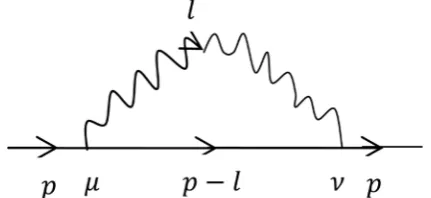
Starting with the Feynman diagram for the one loop correction to the fer-mions line shown in Figure 1 which is represented by

(

∑

( )

p

)

:

Using the standard Feynman rules one can write

(

_∑

( )

p

)

as,

( )

(

)

( )

(

)

(

)

3 2

3 2 2 2

d 2π

p l m l

p ie

p l m l

µ µ

γ

/ − −/

γ

= −

 _/ ₋_/ ₋ 

 

∑

∫

[image:4.595.265.481.606.705.2]

Using the Feynman identity for combining the denominators, we can write

(5)

( )

(

)

( )

(

)

(

)

(

)

1 3 2

3 ₂ 2

2 2

0 d d

2π ₁

p l m l

p ie x

p l x m x l x

µ µ

γ _/ − −/ γ

= −

 ₋ ₋ ₊ ₋ 

 

∑

∫ ∫

Shifting the variable of integration as l l px′ = − _{and simplifying we get}

( )

(

)

_{( )}

(

)

(

)

1 3

2

3 ₂ ₂ ₂ 2

0

1 d

d

2π 1

p x m l

l

p ie x

l m x p x x

µ µ

γ

 − − − ′/

γ

′ / 

= −

′ − + − 

 

∑

∫ ∫

The term linear in l′_{integrates to zero because of symmetric integration, so}

( )

(

)

_{( )}

(

)

(

)

1 3

2

3 ₂ ₂ ₂ 2

0

1 d

d

2π 1

p x m

l

p ie x

l m x p x x

µ µ

γ

__/ − − _

γ

= −  − + −   

∑

∫ ∫

(2.1.1)

Which is taken as the common starting point for both Dimensional and Op-erator regularization.

Using Feynman identity and then γ-algebra, the above result becomes,

( )

(

)

( )

(

)

(

)

(

)

( )

(

)

(

)

1 2

2 ₂ ₂ 1 2

0 1 2 2 1 2 2 2 0 1 3

π ₂ _π _d

4π ₁

1 3

d

8π ₁

p x m

e

p x

m p x x

p x m

e _x

m p x x

µ

_µ

µ

− +     =  − −    − + _/    =  − −   

∑

∫

(2.1.2)

Thus according to dimensional regularization, we see that there is no diver-gent part in (2 + 1)-dimensional space-time, because the integrals are finite in 3-dimensions.

2) Operator Regularization Method:

The same one-loop correction to fermion can be evaluated using OR, follow-ing the rule cited in Equations (2.5) and (2.6) in ref. [8]. The amplitude of the self-energy diagram as

( )

(

)

( )

(

)

(

)

(

)

1 3 2 3 2

0 2 2 2

0

1 1

d d

d lim

d ₂_π ₁

p

p x m

l

ie x

l m p x x

µ µ

ε ε

ε αε γ γ

ε + → + __/ − − _ = −  − + −   

∑

∫

Using the standard integral

( )

₍

₎

( ) ( )

(

)

( )

2

2 ₂ ₂ ₂

d 1 1

2π 4π

w

w A w A w

A w l

A

l M M −

Γ −

=

Γ +

∫

(2.1.3)

we get,

( )

(

)

( )

(

)

(

)

(

)

₍

₎

1 2 3 2 0 1

0 ₂ ₂

2 d 1 4π 1 1 d 2 lim . d 2 1 ie

p x p x m

m x p x x

µ µ ε ε γ γ ε ε αε ε ε → + − = __/ − − _

 _Γ ₊  

(6)

(

)

(

)

₍

₎

(

)

(

)

1 0

2 2 2

1 2 0 1 1 d 2

Here, lim .

d 2 1 1 1 ! d 2 lim

d 1 !

m x p x x

u ε ε ε ε ε ε αε ε ε

ε αε ε

ε ε → +   − +_ _   →

 _Γ ₊  

   ₊ _ _    Γ +   − + −      _ _  + −  _ _      = _ _ +      

(

)

( )

(

)

(

)

(

)

(

)

(

)

(

)

(

)

2 2 1 1 2 2 0 1 1 2 2

where 1

1 ₁ 1 _!

2 2

lim

1 ! 1 !

1 1 1

1 !ln 1

2 2 2

1 ! 1 !

u m x p x x

u u

u u u F

ε ε

ε

ε ε

εα ε αε ε

ε ε

ε αε ε ε εα ε ε

ε ε     − +_ _ − +_ _ →     − +_ _ − +_ _     = − + −  _ _ _ _ − + + −  _ _ _ _      = _ + + +        

+ _ − _ + Γ_ + _{ } + _

      − + + +

(

)

(

) (

)

(

)

1 2 1 2 1

1 ! 2 2

π 2 1 ! u F u ε

ε εα ε ε ε

ε

 

− +_ _   

+ _ − _ Γ + + 

   − _= +   Therefore,

(

)

(

)

₍

₎

1

₍

₎

1 2

0 ₂ ₂ 2 2

2 1 1

d 2 π

lim .

d 2 ₁

1 p x x m x

m x p x x

ε ε

ε

ε αε

ε ε

→ +

 _Γ ₊  

   ₊ _ _    = Γ +  ₋ ₊ ₋ _{ }_ − − _     (2.1.4)

Thus Equation (2.1.4) becomes,

( )

(

)

( )

(

)

(

)

( )

(

₍

)

₎

1 2

3 2 ₂ ₂ 1 2

0 1 2 1 2 2 2 0 π

d 1 3

4π ₁

1 3

d

8π ₁

ie

p x p x m

p x x m x

p x m

e _x

m p x x

− = __/ − + _  − −    − +   − /  =  − −   

∑

∫

This is the same form as like as obtained by dimensional regularization ap-proach.

2.2. One Loop Photon Correction in (2 + 1) Dim.

Using Dimensional and Operator Regularizations

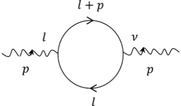
Let us consider the Feynman diagram for the one loop correction to the photon line shown in Figure 2 which is represented by Πµν

( )

p :

The QED one loop correction to the photon line in (2 + 1)-dimensions is

( )

(

) (

)

(

)

(

)

3 2

3 2 2 2 2

d 2π

l p m l m

l

p e Tr

l p m l m

µ ν µν

γ

 _/_{+ −} _/₋  /  

Π = _ _

 ₊ ₋  ₋

  

 

(7)

[image:7.595.280.467.71.181.2]

Figure 2. One loop Feynman diagram for external boson lines.

Combining the denominator using the Feynman identity and simplifying, we get

( )

(

) (

)

(

)

(

)

(

)

1 3

2

3 ₂ ₂ ₂ ₂ 2

0 d d

2π ₁

Tr l p m l m

l

p e x

l p x m x l m x

µ ν

µν

γ γ

 /+ −_/ /− 

 

Π =

 ₊ ₋ ₊ ₋ ₋ 

 

∫ ∫

(2.2.1)

Now putting l l px′ = + _{in Equation (2.2.1), then we get,}

( )

(

) (

)

(

)

(

)

(

)

(

)

1 3

2

3 ₂ ₂ 2

2 2

0

d d

2π ₁ ₁

Tr l px p m l px m l

p e x

l p x x m x l px m x

µ ν

µν

γ ′ γ ′

 / − + − / − − 

′  / / / 

Π =

 _′₊ ₋ ₋ ₊ _′₋ ₋ ₋ 

 

 

∫ ∫

After simplification Equation (2.2.1) with l′ →l becomes,

( )

_{

₍

₎

_}

(

)

(

)

(

)

{

}

{

(

)

}

1 3

2

3 ₂ ₂ ₂ 2

0

2

2 2 2 2

2 2 2

2 d

4 d

2π 1

2 1

1 1

l l l

p e x

l m p x x

x x p p p

l m p x x

µ ν µν

µ ν δµν δµν

 

Π = _

− + −





− −



− −



− + −

− + − _

∫ ∫

(2.2.2)

If we apply the following integrals in the first and third terms in the integrand of Equation (2.2.2),

(

)

(

)

(

)

2 2

2

2 2

2

2 2

I) d

2

π 1 1 ₁

2 2 2

d

l l l

l lq m

i _{q q} d _g _q _m d

q m

µ ν α

µ ν µν

α α α

α −

+ −



  

= Γ − + − − Γ_ − − _

  

− −

∫

II)

(

)

( )

(

)

2

2 2 2 2

2 1

d 1 π

2

d d

d

l i

l lq m q m

α

α α

α

α −

Γ −

= −

+ − Γ − −

∫

We arrive at,

( )

(

)

( )

(

)

(

)

{

}

1 3

2 2

3 ₂ ₂ ₂ 2

0

1 d

8 d

2π ₁

x x

l

p e p p p x

l m p x x

µν µ ν

δ

µν

 ₋ 

 

Π = − _ _

− + −

 

∫ ∫

(2.2.3)

Which is again taken as the common starting point for both Dimensional and Operator regularization for one loop correction to the photon lines.

(8)

( )

(

)

( )

(

)

(

)

(

)

( )

₍

(

₎

)

2

2 2 1 2 2

3 2 2

0

2 _{2 1}

1 2

2 2

0

8 ₁

d 1

2π 2π

8 ₁

d

2π ₁

ie p p p p x x m

p xx x

ie p p p x x

x

p x x m

ε µ ν µν

µν

µ ν µν

δ

µ

δ

−

− −  − − 

Π = −  

 

 

− − ₋

=

 − − 

 

∫

(2.2.4)

Thus according to dimensional regularization, we see that there is no diver-gent part in (2 + 1)-dimensional space-time, because the integrals are finite in 3-dimensions.

Now proceeding with operator regularization and again following the same route, we get,

( )

(

)

( )

(

) (

)

(

)

1 3

2 2

3 2

0 2 2 2

0

1 1

d d

8 d lim

d 2π 1

x x

l

p e p p p x

l m p x x

µν µ ν µν _ε ε

ε αε

δ

ε +

→

+ −

Π = − −

 − + − 

 

∫

(2.2.5)

Performing the momentum integral (2.1.3), so that relative to the Equation (2.2.5) we get, A= +

ε

2_, 3

2

w= , _M2 _{= −}_m2₊_{p x}2

(

₁₋_x

)

_{, then Equation (2.2.5)} becomes,

( )

(

)

(

)

(

)

(

)

₍

₎

1

2 2

3 2

0

1 0

2 2 ₂

1

8 d 1

4π

1 1

d 2

lim .

d 2

1

p e p p p x x x

m p x x

µν µ ν µν

ε ε

δ

ε

ε αε

ε ε

→ +

Π = − − −

 _Γ ₊  

 

 ₊ _ _ 

 

⋅

Γ +

 ₋ ₊ ₋ 

 

 

∫

Now using the Equation (2.1.4) then above equation reduces to,

( )

(

)

(

)

(

)

(

)

( )

₍

(

₎

)

2 2

3 2 ₂ ₂ 1 2

2 _{2 1}

1 2

2 2

0

1 π

8 1

4π 1

4 ₁

d

2π ₁

p e p p p x x

p x x m x

e p p p x x

x

p x x m

µν µ ν µν

µ ν µν

δ

Π = − − −

 − − 

 

− − ₋

=

 − − 

 

∫

This is the same form as we obtained by dimensional regularization approach.

2.3. One Loop Vertex Correction in (2 + 1) Dim. Using

Dimensional and Operator Regularizations

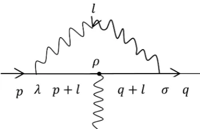
Let us now consider the Feynman diagram for the one loop correction to the vertex shown in Figure 3 which is represented by Γρ

(

p q,

)

.

The QED one loop correction to the vertex in (2 + 1)-dimensions is

(

)

( )

(

)

(

)

(

)

(

)

( )

(

) (

)

(

)

(

)

3

3 2

3 3

3 2 2 2 2 2

d ,

2π

d 2π

l i i

p q ie ie ie

p l m q l m l

ie

l p l m q l m

τσ

ρ λ ρ σ

λ ρ λ

δ

γ γ γ

 

Γ =  − − − 

/ /

+ + + +

 / / 

 

 _/+ −/ _/+ −/ 

 

= −

 ₊ ₋   ₊ ₋ 

   

∫

(2.3.1)

(9)

[image:9.595.274.471.68.195.2]

Figure 3. One loop Feynman diagram for vertex function.

and shifting the variable of integration l→ +l px qy+ _{and simplify the} deno-minator and numerator, we obtain,

(

)

( )

(

)

(

)

(

)

(

)

(

)

(

)

1 1 3

3

0 0

3

2 2 2 2

d

, 2 d d

2π

1 1

1 1 2

x _l

p q ie x y

l p x qy m l q y px m

l m x y p x x q y y p qxy

ρ

λ ρ λ

γ γ γ

−

Γ = −

 /+ _/ + +_/ − /+_/ + + _/ − 

 

⋅

 − + + − + − − ⋅ 

 

∫ ∫ ∫

This integral contains convergent and divergent pieces. The part of the nu-merator quadratic in l is divergent, the rest convergent, so separating the diver-gent piece ( )1

₍

_{p q}_,

₎

ρ

Γ and convergent piece ( )2

₍

_{p q}_,

₎

ρ

Γ , i.e.

(

_{p q}_,

)

( )1

₍

_{p q}_,

₎

( )2

₍

_{p q}_,

₎

ρ ρ ρ

Γ = Γ + Γ

Thus the divergent piece is,

( )

₍

₎

( )

₍

₎

1 1 3

1 3

3 ₂ ₂ 3

0 0

d

, 2 d d

2π

x _l _{l l}

p q ie x y

l M

σ ρ σ ρ

γ γ γ

− _{/ /}

Γ = −

−

∫ ∫ ∫

(2.3.2)

where, _M2_≡_{m x y}2

(

₊

)

₋_{p x}2

(

₁₋_x

)

₋_{q y}2

(

₁₋_y

)

₊₂_{p qxy}_⋅ _.

Which is taken as the common starting point for both Dimensional and Op-erator regularizations for one-loop correction to the vertex.

Using Feynman identity and then γ-algebra, the above result becomes,

( )

₍

₎

( )

_{( )}

( )

_{( )}

( )

_{( )}

3

1 1 1

2 ₂ 1 2

0 0

3 1 1

2 ₂ 1 2

0 0 3 1 1

1 2 2 0 0

1 2

2

, d d

4π

2 π _d _d 1 4π

1 d d 4π

x

e

p q x y

M e

x y M e

x y M

ρ ρ

ρ

µ _γ

µ γ

µγ

−

  Γ   

Γ =

=

∫ ∫

(2.3.3)

where, _M2_≡_{m x y}2

(

₊

)

₋_{p x}2

(

₁₋_x

)

₋_{q y}2

(

₁₋_y

)

₊₂_{p qxy}_⋅ _.

(10)

( )

₍

₎

( )

(

)

₍

₎

1 1 3

1 3

3 3

0 2 2

0 0

d d

, 2 d d lim 1

d 2π

x _l _{l l}

p q ie x y

l M

σ ρ σ

ρ _ε ε

γ γ γ

ε αε

ε

−

+ →

/ /

Γ = − +

−

∫ ∫

∫

Now performing the momentum integral -I from above, then we get,

( )

₍

₎

( )

(

)

(

)

_{( )}

1 1

2 1

3 2 ₀ 1

2

0 0 2

1 1

d 2

, d d lim

d 3

4π

x

e

p q ie x y

M

ρ _ε σ λ ρ τ σ

ε

ε αε

γ γ γ γ γ

ε ε

−

→ +

 _Γ ₊ 

 

 ₊ _ _

 

Γ = − ⋅

Γ +

 

 

∫ ∫

Now using the Equation (2.1.4) and γ-algebra, then above equation reduces to,

( )

₍

₎

( )

2

1 1 1 1

2 1

3 2 ₂ 1 2 ₂ 1 2

0 0 0 0

π 1

, d d d d

16π

4π 2

x _e x

e

p q ie x y ie x y

M M

ρ

ρ ρ

γ

− −

Γ = − = −

   

   

∫ ∫

(2.3.4)

where, _M2_≡_{m x y}2

(

₊

)

₋_{p x}2

(

₁₋_x

)

₋_{q y}2

(

₁₋_y

)

₊₂_{p qxy}_⋅ _.

This is the same form as like as obtained by dimensional regularization ap-proach.

3. Path Integral Form of Operator Regularization

for One Loop Generating Functional in QED

The path integral form of OR for one-loop case is described in ref. [15]. That is if we consider the QED Lagrangian as,

(

)

2

(

)

(

)

2

1 1

4 2

L i µ e µ m µ

µ µ ν ν

γ

µ

γ

µ

_α

µ

= − ∂ Ω − ∂ Ω + Ψ − ∂ − Ω − Ψ − ∂ Ω _(3.1)

and let us expand this Lagrangian taking background field quantization of the fields in the following form, gauge field

Ω

µ and fermionic field

ψ

are

re-spectively,

V Q

µ µ µ

Ω =

+

_{, for gauge field}

Ω

_µ

q

ψ η= + , for fermionic field

ψ

,

where

V

µ and

η

are the classical fields and

Q

µ and q are the quantum

fields.

Therefore Equation (3.1) becomes,

(

)

(

)

(

)

(

)

(

)

2

1 4

1 2

L V Q V Q

q i e V Q m q

V Q

µ µ µ µ ν ν ν ν

µ µ

µ µ µ

µ µ µ µ

η γ γ η

α

= − ∂ + ∂ − ∂ − ∂

+ + − ∂ − + − +

− ∂ + ∂

(

) (

)

(

)

(

)

(

)

(

)

(

)

2

1 4

1 2

Q Q V V i m

i m q q i m

e V V q Q Q q q V

q V q q Q q Q q V Q

µ

µ µ ν ν µ µ ν ν µ

µ µ

µ µ µ µ µ

µ µ µ

µ µ µ µ µ µ µ

η γ η

η γ γ η

ηγ η ηγ ηγ η ηγ γ η

γ γ η γ

α

 

= _ ∂ − ∂ + ∂ − ∂ _ + − ∂ −

+ − ∂ − + − ∂ −

+ + + + +

+ + + − ∂ + ∂

(11)

DOI: 10.4236/jamp.2018.610175 2077 Journal of Applied Mathematics and Physics Following ref. [7] the one-loop generating functional for Green’s functions 1

Z is

1

1 2 2 2 1 2 1

det det

det 1

D A

Z

B p δµν _α p p eµ ν ηγµD−γ ην eηγνD−γ ηµ

/

= =

 _{− −}  ₋ _/ ₋ _/ 

 

 _ _ 

 

(say) (3.3)

where, D µ

(

i eV

)

p eV

µ µ

γ

/ = − ∂ − = − /_/

Here we see that Z1 is the ratio of determinant of operators. Each of the de-terminants occurring in Equation (3.3) requires regularization and a corres-ponding ξ-function. The numerator and denominator separately contribute to Green’s functions with only external boson lines and with both external fer-mions lines and vertex function in massless QED respectively.

3.1. One-Loop Generating Functional and Loop Corrections for

External Boson Lines

To find the loop corrections or to write the generating functional for external boson lines one has to make a close look at the numerator of Equation (3.3) and on the other hand for external fermion lines one has to take care of the denomi-nator of Equation (3.3). So for bosonic case we have to regulate the detA

through the use of ξ-function in Equation (2.5a) yielding

( )

/

1 ₀

det_{A Z}A exp lim A

ε→ ξ ε

 

= = _− _

(3.1.1) where,

( )

_{( )}

1

(

)

0

1 _d_{t t tr}ε _exp _t

ξ ε ε

∞ −

= −Ω

Γ

∫

with Ω = − /p eV/ . (3.1.2)

As we mentioned in Section-2, after regularization we have to consider Schwinger expansion, to this view let us now identify the operator Ω0 and ΩI with p/ and − /eV, respectively, then by Equation (2.4), Equation (3.1.1) can be written as,

( )

(

)

( )

₍

₎

₍

₎

( )

₍

₎

( )

₍

₎

₍

₎

2 1

1 ₀

0 1

1 0

1 1 3

1 1

0 0

d 1 exp lim d

d 2

d

d d 3

A pt pt

u pt upt

u pt u v pt uvpt

t

Z t t tr e te eV

u e eV e eV

t _{u u v e} _{eV e} _{eV e} _eV

ε

ε ε ε

∞

− −/ −/ →

− − / −/

− − / − − / − /

  

= − _Γ  − + − /



  



⋅ − / − /

  

− − / − / − / + 

 

∫



(3.1.3)

To one-loop order this series plays the same role as Feynman rules in the usual perturbation theory. Here we want to evaluate the one-loop correction to the two-point function for external photon in QED; we restrict our attention to the term bilinear in

V

µ on the right-hand side of Equation (3.1.3). This leaves

us with

( )

1

2 1

1

1 ₀

0 0

d

exp lim d d

d 2

u pt

A upt

VV e t

Z _ε t ε tr ue Ve V

ε ε

∞ +

− − / −/ →

   

= − _Γ  / /

 

   

(12)

DOI: 10.4236/jamp.2018.610175 2078 Journal of Applied Mathematics and Physics Now let us complete the functional trace

( ) 1

1 0

d u pt upt

T tr₌ _ ue− − /Ve V_/ −/ _/_



∫

 (3.1.5)

Schwinger has pointed out that such traces are most easily evaluated in mo-mentum space. We introduce a complete orthonormal set of states p/ that are

eigenstates of the operator

p

µ, where, in n dimensions,

( )

₂_π 2

ip x n

e

x p_/ = /⋅ (3.1.6a) and

(

)

( )

2

2π n

f p q p f q = / −/

/ / (3.1.6b)

On the right-hand side of Equation (3.1.6b), f p q

(

_/ −_/

)

is the Fourier trans-form of f x

( )

:

(

)

( )

2

( )

d 2π

n

ix p q n

x

f p q₋ ₌ f x e− ⋅ −/ /

/ /

∫

(3.1.7)

Equation (3.1.5) takes the form,

(1 )

3 3 3 3

d d d d u pt upt

T ₌

∫

p q r s p e_/ _/ _/ _/ _/ − − / q q V r r e_{/ /} _/ _{/ /} −/ s s V p_{/ /} _/ _/

(3.1.8) Upon inserting the complete set ₁₌ _d3_{p p p}

/ / /

∫

at the appropriate places,

and using (3.1.6), we rewrite Equation (3.1.8) as,

(

)

( )

(

)

(

)

( )

(

)

( )

(

) (

)

. 1

3 3 3 3

3 2 3 2

3 3 1 3

d d d d

2π 2π

d d 2π

ir q u pt

is p urt

u pt uqt

V p q e

T p q r s e r q

V r s _e e _{s p} p q e V p q V q p

δ

/ / − − /

⋅/ / − /

− − /−/

− / / /

= / / / / ⋅ /−/

− / / /

⋅ ⋅ _{/ /}−

/ /

= / _{/ /}− / _{/ /}−

∫

(3.1.9)

After shifting the variable of integration p_/ → +p q_/ _/ , Equation (3.1.9) be-comes,

( )

( ) ( )

3 3 1 3

d d 2π

q u p t

p q

T₌

_∫

e− + −/ /V p V_/ _/ ₋p _(3.1.10)

Upon substituting Equation (3.1.10) into Equation (3.1.4), we find that

( )

1AVV exp lim₀ VVA

Z _ε ξ ε

→

 _′ 

= _− _ (3.1.11a)

where,

( )

_{( )}

( ) ( )

( )

1

2 3

1

1 3

3

0 0

d d d d

2 2π

q u p t A

VV e t tε u pV p V p q e

ξ ε

ε ∞

− + − 

+  /

= / / −

Γ

∫

∫ ∫

∫

(3.1.11b)

(13)

( )

(

_{( )}

)

( ) ( )

( )

(

)

(

)

2

2 1 3

3

3 ₂ 2

2 2

0

1

2 _d _d d

2 2π ₁

A VV

q u p

e _{pV p V p} _u q

q u p

ε ε

ε

ξ

ε

+ + − −  

Γ + / /

= / / −

Γ _ _{− −} _

 

∫

∫ ∫

(3.1.12)

Now the last integral I1 (say) of Equation (3.1.12) can be calculated as fol-lows:

( )

(

)

(

)

( )

(

)( ) (

)

(

) ( )

(

)

2 3

1 3 ₂ ₂ ₂ 2

1 2 2

2 3

3 ₂ ₂ ₂ 2

1 d

2π ₁

2 1 1

d

2π ₁

q u p

q I

q u p

q q u p u p

q

q u p

ε

ε ε ε

ε ε + + + + + ∈+ + − − _/ _/   =  _{− −}    _/ ₋ ₊ _/ ₋ _/ _{+ + −} _/    =  _{− −}   

∫



Differentiating Equation (3.1.12) with respect to ε_{and taking}

ε

→0_{, we} see that the product terms in ε will vanish. Hence in the numerator of I1 only the first and last term will contribute.

( )

(

)

(

)

(

) ( )

)

2

2 2 2 2

3

1 3 ₂ 2 ₂ 2

2 2 2 2

1 d

2π ₁ ₁

q _u _p

q I

q u p q u p

ε ε ε ε ε + + + + +   −  / /  ∴ = _ + _  _/ − − _/ − −   

∫

(3.1.13)

To evaluate this integral let us consider the standard integral,

( )

(

) (

)

( )

2 2 ₂ 4

2 2 2

d 1 2 2

2π ₁₆_π

2 r

n

n _{r m}

n m n

n n

r m r

q

q _c

n

q c _m

 + −    

   

Γ_ + _{ }Γ − − _

   

=

 

+ _Γ_{ }_Γ

 

∫

(3.1.14)

Using Equation (3.1.14) in Equation (3.1.13), we get,

(

)

{

(

)

}

( )

(

)

(

) ( )

{

(

)

}

(

)

( )

(

) ( ) (

) ( )

3 2 ₂ 2 2 2 2 1 ₂ 3 4

3 0 2

2 2 2 2 2

1 ₁ ₁

2 3 2

2 3 ₂ 2 3

1 ₁ 2 2 2 2

3

16π ₂

2

3 ₂ 3

2 2

1 1

3 ₂ 2

1 1 ₁ ₁ 2 5

2 π 2 2

4π

I u p

u p u p

u p

ε _ε

ε

ε ε

ε _ε _ε

ε _ε ε

ε ε ε ε ε +  ₊ _{− +}       _{+ − −}   + + _ _ − ₋ ₋

 _Γ + ₊  _Γ _{+ −} + ₋ 

   

 _ _{ } _



= − −

 

 _Γ _Γ ₊

 

 _{ }





   

Γ_{  }Γ + − _{ }

   _{ }

+ − _/ − − ⋅

  

Γ_{ }Γ + _

  

 

= − − Γ_ +

Γ +  

( )

1

(

) ( ) ( )

1 2 (2 1) 2 1 2 2 1 1 1 2

u p p

ε ε ε ε

ε

ε  

− +_ _ − + − +

 _Γ ₋ 

  

 _ _





 

+ − − _/ Γ_ + _

 

Thus Equation (3.1.12) becomes,

( )

(

)

( ) ( )

(

)

( ) ( )

( )

(

) ( )

( )

(

) ( ) ( )

( )

2 1 1

3 _{2 2}

3 2

0

1 1

1 ₁ ₂ _{2 1}

2

2 1 1 _d _d ₁

2 ₄_π 2

2 5 1

1

2 2 2 2

π 1 1 1 2 A VV e

pV p V p u

u p

u p p

ε

ε ε

ε ε ε ε

ε ξ ε ε ε ε ε ε − − −   − +_ _ − + − +  

Γ + 

= / / − _ −

Γ Γ + 

   

⋅ − Γ_ + _{ }Γ − _

   



 

+ − − _/ Γ_ + _

 

(14)

( )

( ) ( ) ( )

( )

( ) ( )

( )

2 1

3 _{2 2}

2

2 1

1 ₂ _{2 1}

2

1 _d ₁ 1

2 8π

3 1 1 1

2 2 2 2 2 2 2 2

π ₁ 1 1

2 2 2

e _{pV p V} _p

p

p p

ε

ε ε ε

ε ε

ε ε ε ε

ε ε − −   − +_ _ + − +    = / / − _ − _ _

Γ   − 

 

     

⋅ _ + _ + _ − _Γ_ − _

 



   

+ − _ _ _/ Γ_ + __

−    _

∫

( ) ( ) ( )

( )

_{( )}

( )

( ) ( )

( )

2 1

3 _{2 2}

2 1

1 ₂ _{2 1}

2 2

1

d 1

2 8π

3 1 1 1

2 2 2 2 2 2 4

π ₁ 1 1 1

2 2 2 2

e _{pV p V} _p p

p p

ε

ε _ε _ε

ε ε

ε ε ε

ε ε ε ε − −   − +_ _ + − +    = / / − _ − _ _ −    Γ     ⋅ _ + _ + _ − _ Γ         

+ − _ ₋ _ / Γ_ + __Γ  

∫

where we have used

( )

2

1

2 4

ε

ε Γ

_Γ −  ₌

   _ _   .

( ) ( ) ( ) ( )

(

₍

₎

)

( )

( ) ( )

( )

3 2

2 1 ₁

3 _{2 2}

2

2 2 1

1 ₂ _{2 1}

2 3 3 d 1 24 2 8π 1 2 2

π ₁ 1

2 2 π 2

e _{pV p V} _p _p

p p

ε _ε

ε

ε ε ε

ε ε ε ε − − −   − +_ _ + − +  + − −  = / / − _ − −    _Γ ₊  _

          + − _ _ _/ _ − Γ   _ 

∫

[Using Duplication formula]

( ) ( ) ( ) ( )

(

₍

₎

)

( )

( ) ( )

( )

(

)

(

)

3 2

2 1 ₁

3 _{2 2}

2

1 ₂ _{2 1}

2 1 2 3 3 d 1 24 2 8π 2 1 1 2 2

e _{pV p V} _p _p

p p

ε _ε

ε ε ε ε

ε ε ε

ε ε ε ε − −   − +_ _ + − + ₋    ₊ _{− −}  = / / − − −   + + − _/ _ − _

∫

where we have used 2 1 2 2 1

(

2 1

)

2 4

ε ε _ε

_Γ +  ₌ + _Γ ₊

   

 _ _ _ _

  .

To see sign of the term, let us put

ε

→0_{in the factor}

( )

1 12 2 ε −

− and

( )

1 ε 12

  − +_ _

− , then these terms are equal to i and –i. Thus the above equation be-comes,

( )

( ) ( ) ( )

(

₍

₎

)

( ) ( )

( )

(

)

(

)

3 2 2 1 3 2

2 2 1 2 1

3 3 d 24 2 8π 2 1 2 2 A

VV ie pV p V p p

p p

ε

ε ε ε

ξ ε ε ε ε ε − + − + −  + − −  = / / − −   + − / ₋  

∫

(3.1.15)

(15)

( )

( ) ( )

( )

( )( )

(

₍

₎

)

( )

(

)

(

) (

)

( )

(

)

( )

( )( )

( )

(

)

(

) ( ) ( )

( )

(

₍

)

_{) ( ) ( )}

( )

_{( )( ) (}

)

(

)

( ) ( )

( )

3 2 2

1 3

2

2 3 2

1

2

2 2 1 2 1 2 2 1

2 2 1

2 1 2 1

2 2 1

3 3 1

d ln 1

24 2

8π

2 3 6 1 3 3 1 1

24 2

2 1

ln 2 ln

2

2 1 2 1

2 2 2 ln 2 2

2 2

2

A

VV ie pV p V p p p

p

p p p p p p

p p

ε

ε ε ε ε ε

ε ε

ε ε ε

ξ ε

ε

ε ε ε ε ε ε

ε

ε ε

ε

ε ε ε ε

ε ε

−

+ − + − + − +

+ − +

− −

+ − +

 ₊ _{− −}



′ = / / − −

− 

 − + − − + − − − 

 

+  

−

 

 

+

+ / / ₋ /

+ +

⋅ − _{+ /}

− −

+ /

∫

(

)(

)

(

)

( )

(

)

2 2 1

2

2 4 1 2 1 2

ε ε ε ε ε

ε

− − + − + − _



− _

Hence

( )

( ) ( )

( )( )

( )

( ) ( )

( )

0

2 3 2

2

2 3 2

0 lim

1 3

d ln 1

24 2

8π

1 5 1 1 1

24 4 2 2

29

d ln

6 128π

A A

VV VV

ie _{pV p V} _p _p _p

p p

p

ie _{pV p V} _{p p} _p

ε

ξ ξ ε

→

′ = ′

  

= / / − _ ⋅ − _− _

 

  −

 

+ ⋅_ _+ _/ ⋅ ⋅ ⋅ _

  

 

= / / − _ − _

 

∫

(3.1.16)

Substituting of Equation (3.1.16) into Equation (3.1.11a) yields our final ex-pression for Z1AVV as,

( ) ( )

( )

2 3

1 2

29

exp d ln

6 128π

A

VV ie

Z = _ pV p V/ / −p p_ p − __

 



∫

 (3.1.17)

This contributes to the to the one–loop generating functional for external bo-sons (photon) lines.

To find one-loop correction for external boson lines from above generating functional, we have to take logarithm on Equation (3.1.17) and then functional differentiation of the expansion with respect to momentum p.

Thus the one-loop correction for the external boson lines is,

( )

2

29 ln

6 128π

ie _p _p 

= _ − _

  (3.1.18)

Hence the result in (3.1.18) is finite and of the same form as we obtained by the diagrammatic form of Operator regularization and Dimensional regulariza-tion methods in Secregulariza-tion-2. In this secregulariza-tion we have shown and explained how one can choose the appropriate terms from the Schwinger expansion for the problem in hand.

3.2. One-Loop Generating Functional and Loop Corrections for

External Fermion Lines and Vertex Function

(16)

regu-DOI: 10.4236/jamp.2018.610175 2082 Journal of Applied Mathematics and Physics late the detB through use of the ξ-function in Equation (3.11a) yielding

( )

1 1 ₀

det exp lim 2

B B

B Z _ε ξ ε

→

 _′ 

= = _− _

 ,

(3.2.1)

where,

( )

_{( )}

1 2

0

2 2

1 _d _exp ₁ 1

1 1

B _{t t tr} _{t p} _{p p}

e e

p eV p eV

ε

µν µ ν

µ ν ν µ

ξ ε δ

ε α

ηγ γ η ηγ γ η

∞

−    

=_Γ − _ − −_ _ 

 

− ₋ _/ − ₋ _/ 



/ / 

∫

(3.2.2)

In Equation (3.2.2) it is understood that the exponential is tr_exp

(

−tB

)

_, where

2 2 2

0

1 1 1

1

I

B p p p e e

p eV p eV

B B

µν µν µ ν µ ν ν µ

µν µν

δ

ηγ

γ η

ηγ

γ η

α

 

≡ − −_ _ − −

− / − /

  / /

≡ +

(3.2.3)

where,

B

0µν is independent of the background field

η

and η, and

B

Iµν is at

least linear in

η

_andη.

Now as before to use Schwinger expansion in this case let us use the Equation (2.4) and then taking bilinear in

η

_andη on the on the right-hand side of Equation (3.2.1), we end up with

( )

(

)

2

1 ₀

0

2 1

1 d 1 1

exp lim d exp 1

2 d

2 B

Z t t tr p p p

t e D

ε

µν µ ν

ε

µ ν

δ

ε ε α

ηγ γ η

∞

→

−

       

= −_  _{ Γ}   − −_ _ 

 



 

 

  

⋅ − / 

 

∫

(3.2.4)

The exponential factor in the trace of Equation (3.2.4) can be simplified using the complete set of orthonormal projections operators:

( )

2

p p T p

p

µ ν µν δµν

 

=_ − _

  (3.2.5a)

( )

p p₂

L p p

µ ν

µν = (3.2.5b)

These allows us to write

( )

e tB0

µν −

as

2 2

2

0

1

exp 1

1 1

!

n

tp tp

n

p p p t

p t T L e T e L

n

µν µ ν

α

µν µν µν µν

δ

α

∞

− −

=

 _{− −}  

 _ _ 

 

  

= _ _ + __ = +

 

 

∑

(3.2.6)

and let us expand _D_/−1_{in powers of the back-ground field in the}_ξ_-function Equation (3.2.4):

1

1 1 1 ₁ 1

1 1 1 1 1 1

D eV

p eV p p

eV eV eV

p p p p p p

−

−  

/ = = _ − / _

− /

/ /  / 

 

=_ + / + / / + _

/ / / / / /