Notes for ECE-320
Winter 2011-2012
Contents
1 Table of Laplace Transforms 5
2 Laplace Transform Review 6
2.1 Poles and Zeros . . . 6
2.2 Proper and Strictly Proper Transfer Functions . . . 6
2.3 Impulse Response and Transfer Functions . . . 6
2.4 Partial Fractions with Distinct Poles . . . 7
2.5 Partial Fractions with Distinct and Repeated Poles . . . 10
2.6 Complex Conjugate Poles: Completing the Square . . . 15
2.7 Common Denominator/Cross Multiplying . . . 19
2.8 Complex Conjugate Poles-Again . . . 21
3 Final Value Theorem and the Static Gain of a System 22 4 Step Response, Ramp Response, and Steady State Errors 24 4.1 Step Response and Steady State Error . . . 24
4.2 Ramp Response and Steady State Error . . . 28
4.3 Summary . . . 31
5 Response of a Ideal Second Order System 33 5.1 Step Response of an Ideal Second Order System . . . 33
5.2 Time to Peak,Tp . . . 34
5.3 Percent Overshoot, PO . . . 35
5.4 Settling Time, Ts . . . 36
5.5 Constraint Regions in the s-Plane . . . . 38
5.6 Summary . . . 45
6 Characteristic Polynomial, Modes, and Stability 47 6.1 Characteristic Polynomial, Equation, and Modes . . . 47
6.2 Characteristic Mode Reminders . . . 48
6.3 Stability . . . 49
6.4 Settling Time and Dominant Poles . . . 49
7 Time Domain Response and System Bandwidth 51 8 Block Diagrams 59 8.1 Basic Feedback Configuration . . . 59
8.2 Mason’s Gain Formula . . . 60
9 Model Matching 67 9.1 ITAE Optimal Systems . . . 69
9.2 Deadbeat Systems . . . 70
10 System Type and Steady State Errors 73
10.1 Review . . . 73
10.2 System Type For a Unity Feedback Configuration . . . 73
10.3 Steady State Errors for Step and Ramp Inputs . . . 74
10.4 Examples . . . 75
11 Controller Design Using the Root Locus 79 11.1 Standard Root Locus Form . . . 79
11.2 Examples . . . 81
11.3 Loci Branches . . . 82
11.4 Real Axis Segments . . . 83
11.5 Asymptotic Angles and Centroid of the Asymptotes . . . 88
11.6 Common Industrial Controller Types . . . 98
11.7 Controller and Design Constraint Examples . . . 100
11.8 Seemingly Odd Root Locus Behavior . . . 124
12 System Sensitivity 127 12.1 Sensitivity to Parameter Variations . . . 127
12.2 Sensitivity to External Disturbances . . . 132
12.3 Summary . . . 133
13 State Variables and State Variable Feedback 134 13.1 State Variable to Transfer Function Model . . . 136
13.2 State Variable Feedback . . . 139
13.3 Controllability for State Variable Systems . . . 144
13.4 Summary . . . 145
16 z-Transforms 146 16.1 Special Functions . . . 146
16.2 Impulse Response and Convolution . . . 146
16.3 A Useful Summation . . . 148
16.4 z-Transforms . . . 151
16.5 z-Transform Properties . . . 153
16.6 Inverse z-Transforms . . . 156
16.7 Second Order Transfer Functions with Complex Conjugate Poles . . . 161
16.8 Solving Difference Equations . . . 165
16.9 Asymptotic Stability . . . 168
16.10Mapping Poles and Settling Time . . . 168
16.11Sampling Plants with Zero Order Holds . . . 170
16.12Final Notes . . . 174
14 Transfer Function Based Discrete-Time Control 175 14.1 Implementing Discrete-Time Transfer Functions . . . 175
14.2 Not Quite Right . . . 175
15 Discrete-Time State Equations 180
15.1 The Continuous-Time State Transition Matrix . . . 180
15.2 Solution of the Continuous-Time State Equations . . . 182
15.3 Computing the State Transition Matrix, eAt . . . 183
15.3.1 Truncating the Infinite Sum . . . 183
15.3.2 Laplace Transform Method . . . 184
15.4 Discretization with Delays in the Input . . . 186
15.5 State Variable to Transfer Function . . . 189
15.6 Poles and Eignevalues . . . 190
16 State Variable Feedback 191 16.1 Pole Placement by Transfer Functions . . . 192
16.2 State Feedback Examples . . . 194
16.3 General Guidelines for State Feedback Pole Locations . . . 196
17 Frequency Domain Analysis 202 17.1 Phase and Gain Margins . . . 202
18 Lead Controllers for Increasing Phase Margin 209 18.1 Algorithm for Controller Design Using Bode Plots . . . 211
18.2 Examples . . . 212
A Matlab Commands i A.1 Figures . . . i
A.2 Transfer Functions . . . i
A.3 Feedback Systems . . . ii
A.4 System Response to Arbitrary Inputs . . . ii
A.5 Changing the Line Thickness . . . iii
A.6 Poles and Zeros . . . iv
A.7 Roots and Polynomials . . . iv
A.8 Root Locus Plots . . . v
1
Table of Laplace Transforms
f
(
t
)
F
(
s
)
δ
(
t
)
1
u
(
t
)
1
s
tu
(
t
)
1
s
2
t
n
−
1
(
n
−
1)!
u
(
t
) (
n
= 1, 2, 3...)
1
s
n
t
n
u
(
t
) (
n
= 1, 2, 3, ...)
n
!
s
n
+1
e
−
at
u
(
t
)
s
+
1
a
te
−
at
u
(
t
)
1
(
s
+
a
)
2
1
(
n
−
1)!
t
n
−
1
e
−
at
u
(
t
) (
n
= 1, 2, 3, ...)
1
(
s
+
a
)
n
t
n
e
−
at
u
(
t
) (
n
= 1, 2, 3, ...)
n
!
(
s
+
a
)
n
+1
sin(
bt
)
u
(
t
)
b
s
2
+
b
2
cos(
bt
)
u
(
t
)
s
s
2
+
b
2
e
−
at
sin(
bt
)
u
(
t
)
b
(
s
+
a
)
2
+
b
2
2
Laplace Transform Review
In this course we will be using Laplace transforms extensively. Although we do not often go from the s-plane to the time domain, it is important to be able to do this and to understand what is going on. In what follows is a brief review of some results with Laplace transforms.
2.1
Poles and Zeros
Assume we have the transfer function
H(s) = N(s) D(s)
where N(s) andD(s) are polynomials in s with no common factors. The roots of N(s) are the
zeros of the system, while the roots of D(s) are the polesof the system.
2.2
Proper and Strictly Proper Transfer Functions
The transfer function
H(s) = N(s) D(s)
is proper if the degree of the polynomial N(s) is less than or equal to the degree of the poly-nomial D(s). The transfer function H(s) is strictly proper if the degree of N(s) is less than the degree of D(s).
2.3
Impulse Response and Transfer Functions
IfH(s) is a transfer function, the inverse Laplace transform ofH(s) is call theimpulse response, h(t).
2.4
Partial Fractions with Distinct Poles
Let’s assume we have a transfer function
H(s) = N(s) D(S) =
N(s) D(s) =
K(s+z1)(s+z2)...(s+zm) (s+p1)(s+p2)...(s+pn)
where we assume m < n (this makes H(s) a strictly proper transfer function). The poles of the system are at −p1, −p2, ... −pn and the zeros of the system are at −z1, −z2, ... −zm.
Since we have distinct poles, pi ̸=pj for alli andj. Also, since we assumed N(s) andD(s) have no common factors, we know thatzi ̸=pj for all i and j.
We would like to find the corresponding impulse response, h(t). To do this, we assume
H(s) = N(s)
D(s) = a1 1 s+p1
+a2
1 s+p2
+...+an 1 s+pn
If we can find the ai, it will be easy to determineh(t) since the only inverse Laplace transform we need is that of s+1p, and we know (or can look up) s+1p ↔ e−ptu(t). To find a
1, we first
multiply by (s+p1),
(s+p1)H(s) = a1+a2
s+p1
s+p2
+...+an s+p1
s+pn and then let s→ −p1. Since the poles are all distinct, we will get
lim s→−p1
(s+p1)H(s) = a1
Similarly, we will get
lim s→−p2
(s+p2)H(s) = a2
and in general
lim s→−pi
(s+pi)H(s) = ai
Example 1. Let’s assume we have
H(s) = s+ 1 (s+ 2)(s+ 3)
and we want to determine h(t). Since the poles are distinct, we have
H(s) = (s+ 1)
(s+ 2)(s+ 3) = a1 1
s+ 2 +a2 1 s+ 3 Then
a1 = lim
s→−2(s+ 2)
(s+ 1)
(s+ 2)(s+ 3) = slim→−2
(s+ 1) (s+ 3) =
and
a2 = lim
s→−3(s+ 3)
(s+ 1)
(s+ 2)(s+ 3) = slim→−3
(s+ 1) (s+ 2) =
−2 −1 = 2 Then
H(s) = −1 1 s+ 2 + 2
1 s+ 3 and hence
h(t) = −e−2tu(t) + 2e−3tu(t)
It is often unnecessary to write out all of the steps in the above example. In particular, when we want to find ai we will always have a cancellation between (s+pi) in the numerator with the (s+pi) in the denominator. Using this fact, when we want to find ai we can just ignore (or
cover up) the factor (s+pi) in the denominator. For our example above, we then have
a1 = lim
s→−2
(s+ 1) (s+ 3) =
−1 1 =−1 a2 = lim
s→−3
(s+ 1)
(s+ 2) =
−2 −1 = 2
where we have covered up the poles associated with a1 and a2, respectively.
Example 2. Let’s assume we have
H(s) = s
2 −s+ 2
(s+ 2)(s+ 3)(s+ 4) and we want to determine h(t). Since the poles are distinct, we have
H(s) = (s
2−s+ 2)
(s+ 2)(s+ 3)(s+ 4) = a1 1
s+ 2 +a2 1
s+ 3 +a3 1 s+ 4 Using the cover up method, we then determine
a1 = lim
s→−2
(s2−s+ 2)
(s+ 3)(s+ 4) = 8
(1)(2) = 4 a2 = lim
s→−3
(s2−s+ 2)
(s+ 2) (s+ 4) =
14
(−1)(1) =−14 a3 = lim
s→−4
(s2−s+ 2)
(s+ 2)(s+ 3) =
22
(−2)(−1) = 11
and hence
Example 3. Let’s assume we have
H(s) = 1
(s+ 1)(s+ 5)
and we want to determine h(t). Since the poles are distinct, we have
H(s) = 1
(s+ 1)(s+ 5) = a1 1
s+ 1 +a2 1 s+ 5 Using the coverup method, we then determine
a1 = lim
s→−1
1
(s+ 5) = 1 4 a2 = lim
s→−5
1
(s+ 1) =
1 −4 and hence
h(t) = 1 4e
−tu(t)− 1 4e
−5tu(t)
2.5
Partial Fractions with Distinct and Repeated Poles
Whenever there are repeated poles, we need to use a different form for the partial fractions for those poles. This is probably most easily explained by means of examples.
Example 4. Assume we have the transfer function
H(s) = 1
(s+ 1)(s+ 2)2
and we want to find the corresponding impulse response, h(t). To do this we look for a partial fraction expansion of the form
H(s) = 1
(s+ 1)(s+ 2)2 = a1
1
s+ 1 +a2 1
s+ 2 +a3 1 (s+ 2)2
Example 5. Assume we have the transfer function
H(s) = s+ 1 s2(s+ 2)(s+ 3)
and we want to find the corresponding impulse response, h(t). To do this we look for a partial fraction expansion of the form
H(s) = s+ 1
s2(s+ 2)(s+ 3) = a1
1 s +a2
1 s2 +a3
1
s+ 2 +a4 1 s+ 3
Note that there are always as many unknowns (the ai) as the degree of the denominator polynomial.
Now we need to be able to determine the expansion coefficients. We already know how to do this for distinct poles, so we do those first.
ForExample 4,
a1 = lim
s→−1
1
(s+ 2)2 =
1 1 = 1
ForExample 5,
a3 = lim
s→−2
s+ 1
s2 (s+ 3) =
−1
(−2)2(1) =−
1 4 a4 = lim
s→−3
s+ 1
s2(s+ 2) =
−2
(−3)2(−1) =
2 9
The next set of expansion coefficients to determine are those with the highest power of the repeated poles.
ForExample 4, multiply though by (s+ 2)2 and lets → −2,
a3 = lim
s→−2(s+ 2)
2 1
(s+ 1)(s+ 2)2 = slim→−2
1
or with the coverup method
a3 = lim
s→−2
1
(s+ 1) =
1
−1 =−1 ForExample 5, multiply though by s2 and lets →0
a2 = lim
s→0s
2 s+ 1
s2(s+ 2)(s+ 3) = lims→0
s+ 1
(s+ 2)(s+ 3) = 1 6 or with the coverup method
a2 = lim
s→0
s+ 1
(s+ 2)(s+ 3) = 1 6 =
1 6
So far we have: for Example 4
1
(s+ 1)(s+ 2)2 =
1
s+ 1 +a2 1 s+ 2 −
1 (s+ 2)2
and for Example 5
s+ 1
s2(s+ 2)(s+ 3) = a1
1 s +
1 6
1 s2 −
1 4
1 s+ 2 +
2 9
1 s+ 3
We now need to determine any remaining coefficients. There are two common ways of doing this, both of which are based on the fact that both sides of the equation must be equal for any value ofs. The two methods are
1. Multiply both sides of the equation by s and let s → ∞. If this works it is usually very quick.
2. Select convenient values of s and evaluate both sides of the equation for these values ofs ForExample 4, using Method 1,
lim s→∞
[
s 1
(s+ 1)(s+ 2)2 ]
= lim s→∞
[
s
s+ 1 +a2 s s+ 2 −
s (s+ 2)2
]
or
0 = 1 +a2+ 0
so a2 = -1.
ForExample 5, using Method 1,
lim s→∞
[
s s+ 1 s2(s+ 2)(s+ 3)
] = lim s→∞ [ a1 s s + 1 6 s s2 −
1 4
s s+ 2 +
2 9
s s+ 3
or
0 = a1+ 0−
1 4+
2 9 so a1 = 14 − 29 = 361
For Example 4, using Method 2, let’s choose s = 0 (note both sides of the equation must be finite!)
lim s→0 [
1
(s+ 1)(s+ 2)2 ]
= lim s→0
[
1
s+ 1 +a2 1 s+ 2 −
1 (s+ 2)2
]
or
1
4 = 1 + a2
2 − 1 4 so a2 = 2(14 +14 −1) =−1
ForExample 5, using Method 2, let’s choose s=−1 (note thats= 0, s=−2, or s=−3 will not work)
lim s→−1
[
s+ 1 s2(s+ 2)(s+ 3)
]
= lim s→−1
[ a1 1 s + 1 6 1 s2 −
1 4
1 s+ 2 +
2 9
1 s+ 3
]
or
0 = −a1+
1 6− 1 4 1 9 so a1 = 16 − 14 + 19 = 361
Then for Example 4,
h(t) = e−tu(t)−e−2tu(t)−te−2tu(t) and for Example 5
h(t) = 1
36u(t) + 1
6tu(t)− 1 4e
−2tu(t) + 2 9e
−3tu(t)
In summary, for repeated and distinct poles, go through the following steps:
1. Determine the form of the partial fraction expansion. There must be as many unknowns as the highest power ofs in the denominator.
2. Determine the coefficients associated with the distinct poles using the coverup method. 3. Determine the coefficient associated with the highest power of a repeated pole using the
4. Determine the remaining coefficients by
• Multiplying both sides bys and letting s→ ∞
• Settingsto a convenient value in both sides of the equations. Both sides must remain finite
Example 6. Assuming
H(s) = s
2
(s+ 1)2(s+ 3)
determine the corresponding impulse responseh(t). First, we determine the correct form
H(s) = s
2
(s+ 1)2(s+ 3) = a1
1
s+ 1 +a2 1
(s+ 1)2 +a3
1 s+ 3 Second, we determine the coefficient(s) of the distinct pole(s)
a3 = lim
s→−3
(s2)
(s+ 1)2 =
9 4
Third, we determine the coefficient(s) of the highest power of the repeated pole(s)
a2 = lim
s→−1
(s2)
(s+ 3) = 1 2 Fourth, we determine any remaining coefficients
lim s→∞
[
s s
2
(s+ 1)2(s+ 3) ] = lim s→∞ [ a1 s s+ 1 +
1 2
s (s+ 1)2 +
9 4
s (s+ 3)
]
or
1 = a1+ 0 +
9 4 ora1 = 1− 94 =−54.
Putting it all together, we have
h(t) = −5 4e
−t
u(t) + 1 2te
−t
u(t) + 9 4e
−3t u(t)
Example 7. Assume we have the transfer function
H(s) = s+ 3 s(s+ 1)2(s+ 2)2
First we determine the correct form H(s) = s+ 3
s(s+ 1)2(s+ 2)2 = a1
1 s +a2
1
s+ 1 +a3 1
(s+ 1)2 +a4
1
s+ 2 +a5 1 (s+ 2)2
Second, we determine the coefficient(s) of the distinct pole(s)
a1 = lim
s→0
s+ 3
(s+ 1)2(s+ 2)2 =
3 (1)(4) =
3 4
Third, we determine the coefficient(s) of the highest power of the repeated pole(s)
a3 = lim
s→−1
s+ 3
s (s+ 2)2 =
2
(−1)(1) = −2 a5 = lim
s→−2
s+ 3
s(s+ 1)2 =
1
(−2)(1) = − 1 2 Fourth, we determine any remaining coefficients
lim s→∞
[
s s+ 3 s(s+ 1)2(s+ 2)2
] = lim s→∞ [ 3 4 s s +a2
s s+ 1 −2
s
(s+ 1)2 +a4
s s+ 2 −
1 2
s (s+ 2)2
]
or
0 = 3
4 +a2+a4 We need one more equation, so let’s set s=−3
lim s→−3
[
s+ 3 s(s+ 1)2(s+ 2)2
]
= lim s→−3
[
3 8
1 s +a2
1 s+ 1 −2
1
(s+ 1)2 +a4
1 s+ 2 −
1 2
1 (s+ 2)2
]
or
0 = −1 4−a2
1 2 −
1
2 −a4− 1 2 This gives us the set of equations
[
1 1
1
2 −1
] [
a2
a4 ]
=
[ −3
4 5 4
]
with solutiona2 = 1 anda4 =−74. Putting it all together we have
h(t) = 3
4u(t) +e
−t
u(t)−2te−tu(t) + −7 4 e
−2t
u(t)− 1 2te
2.6
Complex Conjugate Poles: Completing the Square
Before using partial fractions on systems with complex conjugate poles, we need to review one property of Laplace transforms:
if x(t)⇔X(s), then e−atx(t)⇔X(s+a) To show this, we start with what we are given:
L{x(t)} =
∫ ∞
0
x(t)e−stdt = X(s) Then
L{e−atx(t)} =
∫ ∞
0
e−atx(t)e−stdt =
∫ ∞
0
x(t)e−(s+a)tdt = X(s+a) The other relationships we need are the Laplace transform pairs for sines and cosines
cos(bt)u(t) ⇔ s s2+b2
sin(bt)u(t) ⇔ b s2+b2
Finally, we need to put these together, to get the Laplace transform pair:
e−atcos(bt)u(t) ⇔ s+a (s+a)2+b2
e−atsin(bt)u(t) ⇔ b (s+a)2+b2
Complex poles always result in sines and cosines. We will be trying to make terms with complex poles look like these terms by completing the square in the denominator.
In order to get the denominators in the correct form when we have complex poles, we need to complete the square in the denominator. That is, we need to be able to write the denominator as
D(s) = (s+a)2+b2
To do this, we always first finda using the fact that the coefficient ofs will be 2a. Then we use whatever is needed to construct b. A few example will hopefully make this clear.
Example 8. Let’s assume
D(s) = s2+s+ 2
and we want to write this in the correct form. First we recognize that the coefficient of s is 1, so we know 2a= 1 or a= 12. We then have
D(s) = s2+s+ 2 = (s+1 2)
To find b we expand the right hand side of the above equations and then equate powers of s:
D(s) = s2+s+ 2 = (s+ 1 2)
2
+b2 = s2+s+1 4 +b
2
clearly 2 =b2+1
4, or b
2 = 7
4, or b =
√
7
2 . Hence we have
D(s) = s2+s+ 2 = (s+1 2)
2+
(√
7 2
)2
and this is the form we need.
Example 9. Let’s assume
D(s) = s2+ 3s+ 5
and we want to write this in the correct form. First we recognize that the coefficient of s is 3, so we know 2a= 3 or a= 32. We then have
D(s) = s2+ 3s+ 5 = (s+ 3 2)
2
+b2
To find b we expand the right hand side of the above equations and then equate powers of s:
D(s) = s2+ 3s+ 5 = (s+ 3 2)
2+b2 = s2+ 3s+9
4 +b
2
clearly 5 =b2+9
4, or b
2 = 11
4, or b =
√
11
2 . Hence we have
D(s) = s2+ 3s+ 5 = (s+3 2)
2+
(√
11 2
)2
and this is the form we need.
Now that we know how to complete the square in the denominator, we are ready to look at complex poles. We will start with two simple examples, and then explain how to deal with more complicated examples.
Example 10. Assuming
H(s) = 1
s2+s+ 2
and we want to find the corresponding impulse response h(t). In this simple case, we first complete the square, as we have done above, to write
H(s) = 1
(s+ 12)2+(√7 2
This almost has the form we want, which is
e−atsin(bt)u(t) ⇔ b (s+a)2+b2
However, to use this form we need b in the numerator. To achieve this we will multiply and divide by b= √27
H(s) = 1
(s+ 12)2+(√7 2
)2
= √1
7 2
√
7 2
(s+ 12)2+(√7 2
)2
or
h(t) = √2 7e
−1
2tsin(
√ 7 2 t)u(t)
The examples we have done so far have been fairly straightforward. In general, when we have complex conjugate poles we will look for a combination of sines and cosines. Specifically, when-ever we have complex conjugate poles, we will assume the correct form for a sine or a cosine
whatever (s+a)2+b2 =
Ab
(s+a)2+b2 +
B(s+b) (s+a)2 +b2
HereA and B are the two unknown coefficients.
Example 11. Assuming
H(s) = s
s2+ 3s+ 5
and we want to find the corresponding impulse response h(t). In this simple case, we first complete the square, as we have done above, to write
H(s) = s
(s+ 32)2+(√11 2
)2
Now we expand using the assumed form for the complex conjugate poles,
H(s) = s
(s+ 32)2+ (√11
2 )
2 =
A√211 (s+ 32)2+ (√11
2 )
2 +
B(s+32) (s+ 32)2+ (√11
2 )
2
Now if we multiply both sides bys and let s→ ∞we get B = 1. Next, if we substitutes=−32 we get
−3 2 11
4
= A
√
which gives A=−3/√11. Now we have all of the parameters we need, and we have
h(t) = e−32tcos( √
11
2 t)u(t)− 3 √
11e
−3
2tsin(
√ 11 2 t)u(t)
Note that it is possible to combine the sine and cosine terms into a single cosine with a phase angle, but we will not pursue that here. The examples we have done so far only contain complex roots. In general, we need to be able to deal with systems that have both complex and real roots. Since we are dealing with real systems in this course, all complex poles will occur in complex conjugate pairs.
Example 12. Assuming
H(s) = 1
(s+ 2)(s2+s+ 1)
and we want to determine the corresponding impulse response h(t). First we need to find the correct form for the partial fractions, which means we need to complete the square in the denominator
H(s) = 1
(s+ 2)(s2+s+ 1) =
1
(s+ 2)((s+ 12)2 + (√3
2 )2)
= A
s+ 2 +
B√23 (s+ 1
2)
2 + (√3
2 )
2 +
C(s+32) (s+1
2)
2+ (√3
2 )
2
Note that we have three unknowns since the highest power of s in the denominator is 3. Since there is an isolated pole at -2, we find coefficient A first using the coverup method
A = lim s→−2
1
(s2+s+ 1) =
1
(−2)2+ (−2) + 1 =
1 3
To find C, multiply both sides by s and lets → ∞, which gives us 0 = A+ 0 +C
which give us C =−A=−1/3. Finally, we substitutes=−1/2 into the equation to get 1
3 2 3 4
= A3
2
+ √B
3 2
3 4 This is simplified as
8
9 =
2 9 +B
3 √ 3 which yields B = √1
3. Finally we have
h(t) = 1 3e
−2tu(t)− 1 3e
−1
2tcos(
√ 3
2 t)u(t) + 1 √
3e
−1
2tsin(
2.7
Common Denominator/Cross Multiplying
As a last method, we’ll look at a method of doing partial fractions based on using a common de-nominator. This method is particularly useful for simple problems like finding the step response of a second order system. However, for many other types of problems it is not very useful, since it generates a system of equations that must be solved, much like substituting values of s will do.
Example 13 Let’s assume we have the second order system
H(s) = b
s2+cs+d
and we want to find the step response of this system,
Y(s) = H(s)1 s
= b
s(s2+bs+c) =a1
1 s +
a2s+a3
s2+bs+c
= b
s(s2+bs+c) =
a1(s2+bs+c) +s(a2s+a3)
s(s2+bs+c)
= b
s(s2+bs+c) =
(a1c)s0+ (a1b+a3)s1+ (a1+a2)s2
s(s2+bs+c)
Since we have made the denominator common for both sides, we just need to equate powers of s in the numerator:
a1c = b
a1b+a3 = 0
a1+a2 = 0
Since c and b are known, we can easily solve for a1 in the first equation, then a2 and a3 in the
remaining equations.
Example 14. Find the step response of
H(s) = 1
s2+ 2s+ 2
using the common denominator method. Y(s) is given by
Y(s) = 1 s
1
s2+ 2s+ 2 =a1
1 s +
a2s+a3
s2 + 2s+ 2
If we put everything over a common denominator we will have the equation 1 = a1(s2+ 2s+ 2) +s(a2s+a3)
Equating powers of s we get a1 = 12, then a3 =−1 anda2 =−12. The we have
Y(s) = 1 2 1 s +
−1
2 s−1
s2+ 2s+ 2
= 1 2 1 s − 1 2
s+ 2 s2+ 2s+ 2
= 1 2 1 s − 1 2
(s+ 1) (s+ 1)2+ 1 −
1 2
1 (s+ 1)2+ 1
In the time-domain we have then y(t) = 1
2u(t)− 1 2e
−tcos(t)u(t)− 1 2e
−tsin(t)u(t)
Example 15. Find the step response of
H(s) = 3
2s2+ 3s+ 3
using the common denominator method. Partial fractions will only work if the denominator is
monic, which means the leading coefficient must be a 1. Hence we rewriteH(s) as
H(s) =
3 2
s2+ 3
2s+
3 2
Y(s) is then given by
Y(s) = 1 s
3 2
s2+ 3
2s+
3 2
=a1
1 s +
a2s+a3
s2 +3
2s+
3 2
If we put everything over a common denominator we will have the equation 3
2 = a1(s
2+3
2s+ 3
2) +s(a2s+a3) = (3
2a1)s
0+ (3
2a1+a3)s
1+ (a
1+a2)s2
Equating powers of s we get a1 = 1, then a2 =−1 anda3 =−32. The we have
Y(s) = 1 s +
−s− 3 2
s2+3
2s+
3 2
= 1
s −
s+34 + 34 s2+3
2s+
3 2
= 1
s −
(s+ 34) (s+3
4)
2+(√15
16
)2 −
3 4 √ 16 15 √ 15 16
(s+34)2 +(√15 16 )
In the time-domain we have then
y(t) = u(t)−e−3t/4cos(
√
15
16t)u(t)− 3 √
15e
−3t/4sin( √
2.8
Complex Conjugate Poles-Again
It is very important to understand the basic structure of complex conjugate poles. For a system with complex poles at−a±bj, the characteristic equation (denominator of the transfer function) will be
D(s) = [s−(−a+jb)][s−(−a−jb)] = [s+ (a−jb)][s+ (a+jb)]
= s2+ [(a−jb) + (a+jb)]s+ (a−jb)(a+jb) = s2+ 2as+a2+b2
= (s+a)2+b2
We know that this form leads to terms of the form e−atcos(bt)u(t) and e−atsin(bt)u(t). Hence we have the general relationship that complex poles at −a±jb lead to time domain functions that
• decay like e−at (the real part determines the decay rate)
3
Final Value Theorem and the Static Gain of a System
The final value theorem for Laplace transforms can generally be stated as follows:
If Y(s) has all of its poles in the open left half plane, with the possible exception of a single pole at the origin, then
lim
t→∞y(t) = lims→0sY(s) provided the limits exists.
Example 1. For y(t) =e−atu(t) witha >0 we have lim
t→∞y(t) = tlim→∞e
−at = 0
lim
s→0sY(s) = lims→0s
1
s+a = lims→0
s
s+a = 0
Example 2. For y(t) = sin(bt)u(t) we have lim
t→∞y(t) = tlim→∞sin(bt) lim
s→0sY(s) = lims→0s
b
s2+b2 = lims→0
sb
s2+b2 = 0
Clearly limt→∞y(t)̸= limssY(s). Why? Because the final value theorem is not valid sinceY(s) has two poles on the jω axis.
Example 3. For y(t) =u(t) we have lim
t→∞y(t) = tlim→∞u(t) = 1 lim
s→0sY(s) = lims→0s
1
s = lims→0
s s = 1
Example 4. For y(t) =e−atcos(bt)u(t) witha >0 we have lim
t→∞y(t) = tlim→∞e
−atcos(bt)u(t) = 0
lim
s→0sY(s) = lims→0s
(s+a)
(s+a)2+b2 = lims→0
s(s+a)
(s+a)2+b2 = 0
One of the common ways in which we use the Final Value Theorem is to compute the static gain of a system. The response of a transfer function G(s) to a step input of amplitude A,
Y(s) = G(s)A s
If we want the final value of y(t) then we can use the Final Value Theorem lim
= lim s→0sG(s)
A s = AG(0) = AKstatic
provided G(0) exists. G(0) is referred to as the gainor static gainof the system. This is a very convenient way of determining the static gain of a system. It is important to remember that the steady state value of a system is the static gain of a system multiplied by the amplitude of the step input.
Example 5. For the transfer function
G(s) = s+ 2 s2+ 3s+ 1
the static gain is 2, and if the step input has an amplitude of 0.1, the final value will be 0.2.
Example 6. For the transfer function
G(s) = s
2+ 1
s3+ 2s2+ 3s+ 4
4
Step Response, Ramp Response, and Steady State
Er-rors
In control systems, we are often most interested in the response of a system to the following types of inputs:
• a step • a ramp • a sinusoid
Although in reality control systems have to respond to a large number of different inputs, these are usually good models for the range of input signals a control system is likely to encounter.
4.1
Step Response and Steady State Error
Thestep response of a system is the response of the system to a step input. In the time domain, we compute the step response as
y(t) = h(t)⋆ Au(t)
whereA is the amplitude of the step and u(t) is the unit step function and ⋆is the convolution operator. In the s domain, we compute the step response as
Y(s) = H(s)A s y(t) = L−1{Y(s)}
The steady state error, ess, is the difference between the input and the resulting response as t→ ∞. For a step input of amplitude A we have
ess = lim
t→∞[Au(t)−y(t)] = A− lim
t→∞y(t)
Note that the steady state error can be both positive (the final value of the output is not as large as the input) or negative (the final value of the output is larger than the input).
Example 1. Consider the system with transfer function H(s) = 4
s2+2s+5. Determine step
re-sponse and the steady state error for this system. First we find the step response,
Y(s) = 4
s2+ 2s+ 5
A s =a1
1 s +
a2s+a3
(s+ 1)2+ 22
= A
[
4 5
1 s −
4
5s+
8 5
(s+ 1)2+ 22 ]
= A
[
4 5
1 s −
4
5(s+ 1)
(s+ 1)2+ 22 −
2 5
2 (s+ 1)2+ 22
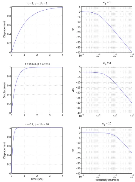
0 1 2 3 4 5 6 0
0.2 0.4 0.6 0.8 1
Time (sec)
Displacement
Input Output steady state error = 0.2
Figure 1: The unit step response and position error for the system in Example 1. This system has a positive position error.
or
y(t) = A
[4
5u(t)− 4 5e
−tcos(2t)u(t)− 2 5e
−tsin(2t)u(t)
]
Then the steady state error is ess = A− lim
t→∞A
[4
5u(t)− 4 5e
−tcos(2t)u(t)− 2 5e
−tsin(2t)u(t)
]
= A− 4A 5
= A
5
The step response and steady state error of this system are shown in Figure 1 for a a unit step (A = 1)input. Note that the positive steady state error indicates the final value of the output is smaller than the final value of the input.
Example 2. Consider the system with transfer function H(s) = (s+1)(1s+3). Determine the step response and steady state error for this system.
First we find the step response,
Y(s) = 5
(s+ 1)(s+ 3) A
s = a1 1 s +a2
1
s+ 1 +a3 1 s+ 3 = 5A
3 1 s −
5A 2
1 s+ 1 +
5A 6
0 1 2 3 4 5 6 7 8 0
0.2 0.4 0.6 0.8 1 1.2 1.4 1.6 1.8 2
Time (sec)
Displacement
Input Output steady state error = −0.667
Figure 2: The unit step response and position error for the system in Example 2. This system has a negative position error.
or
y(t) = A
[5
3u(t)− 5 2e
−tu(t) + 5 6e
−3tu(t)
]
Then the steady state error is
ep = A− lim t→∞A
[
5 3u(t)−
5 2e
−t
u(t) + 5 6e
−3t u(t)
]
= A−5A 3 = −2A
3
The step response and steady state error of this system are shown in Figure 2 for a a unit step (A= 1)input. Note that the negative steady state error indicates the final value of the output is larger than the final value of the input.
Now, as much as I’m sure you like completing the square and doing partial fractions, there is an easier way to do this. We already have learned that if Y(s) has all of its poles in the open left half plane (with the possible exception of a single pole at the origin), we can use the final value theorem to find the steady state value of the step response. Specifically,
lim
= lim s→0s
[
H(s)A s
]
= lim
s→0AH(s)
= AH(0)
and then, for stable H(s) we can compute the steady state error as ess = A−AH(0)
where A is the amplitude of the step input. For a unit step response A = 1.
Example 3. From Example 1, we compute
ess = A−AH(0) = A−A4
5
= A
5
Example 4. From Example 2, we compute
ess = A−AH(0) = A−A5
3 = −2A
3
There is yet another way to compute the steady state error, which is useful to know. Let’s assume we write the transfer function as
H(s) = nms m+n
m−1sm−1+...+n2s2+n1s+n0
sn+d
n−1sn−1+...+d2s2+d1s+d0
To compute the steady state error for a step input we need to compute ess = lim
s→0A[1−H(s)]
Let’s write 1−H(s) and put it all over a common denominator. Then we have
1−H(s) = (s n+d
n−1sn−1+...+d2s2+d1s+d0)−(nmsm+nm−1sm−1+...+n2s2+n1s+n0)
sn+d
n−1sn−1+...+d2s2+d1s+d0
= ...+ (d2−n2)s
2+ (d
1 −n1)s+ (d0−n0)
sn+d
n−1sn−1+...+d2s2+d1s+d0
Then
ess = lim
s→0A[1−H(s)]
Example 5. From Example 1, we have n0 = 4 and d0 = 5, so the steady state error for a step
input isess=A5−54 = A5.
Example 6. From Example 2, we have n0 = 5, d0 = 3, so the steady state error for a step
input isess=A3−35 = −23A.
4.2
Ramp Response and Steady State Error
The ramp response of a system is the response of the system to a ramp input. In the time domain, we compute the ramp response as
y(t) = h(t)⋆ Atu(t)
where A is the amplitude of the step and u(t) is the unit step function. In the s domain, we compute the step response as
Y(s) = H(s)A s2
y(t) = L−1{Y(s)}
The steady state error, ess, is the difference between the input ramp and the resulting response as t→ ∞,
ess = lim
t→∞[Atu(t)−y(t)]
It should be clear that unlessy(t) has a term likeAtu(t), the steady state error will be infinite.
Note that the steady state error can be both positive (the final value of the output is not as large as the input) or negative (the final value of the output is larger than the input).
Example 7. Consider the system with transfer function H(s) = s+11 . Determine the ramp response and steady state error for this system.
First we find the ramp response
Y(s) = 1 s+ 1
A
s2 = a1
1 s +a2
1 s2 +a3
1 s+ 1
= A
[
−1 s +
1 s2 +
1 s+ 1
]
or
y(t) = A[−u(t) +tu(t) +e−tu(t)] Then the steady state error is
ess = Atu(t)− lim t→∞A
[
−u(t) +tu(t) +e−tu(t)] = At−At+A
Example 8. Consider the system with transfer function H(s) = s2+2s+2s+2. Determine the ramp
response and steady state error for this system. First we find the ramp response
Y(s) = s+ 2 s2+ 2s+ 2
A
s2 = a1
1 s +a2
1 s2 +
a3s+a4
s2+ 2s+ 2
= A [ −1 2 1 s + 1 s2 +
1 2
s (s+ 1)2+ 1
] = A [ −1 2 1 s + 1 s2 +
1 2
s+ 1 (s+ 1)2+ 1 −
1 2
1 (s+ 1)2+ 1
]
or
y(t) = A
[
−1
2u(t) +tu(t) + 1 2e
−t
cos(t)u(t)− 1 2e
−t
sin(t)u(t)
]
Then the steady state error is
ess = Atu(t)− lim t→∞A
[
−1
2u(t) +tu(t) + 1 2e
−t
cos(t)u(t)− 1 2e
−t
sin(t)u(t)
]
= At−At+1 2A
= A
2
The ramp response and steady state error for this system are shown in Figure 3 for a a unit ramp input. Note that the steady state error is positive, indicating the output of the system is smaller than the input in steady state.
We can try and use the Final Value Theorem again, but it becomes a bit more complicated. We want to find
ess = lim
t→∞[Atu(t)−y(t)] = lim
s→0s [
A s2 −
A s2H(s)
]
= lim s→0
A
s [1−H(s)] Let’s assume again we can write the transfer function as
H(s) = nms m+n
m−1sm−1+...+n2s2+n1s+n0
sn+dn
−1sn−1+...+d2s2+d1s+d0
If we compute 1−H(s) and put things over a common denominator, we have
1−H(s) = (s n+d
n−1sn−1+...+d2s2+d1s+d0)−(nmsm+nm−1sm−1+...+n2s2+n1s+n0)
sn+d
n−1sn−1+...+d2s2+d1s+d0
= ...+ (d2−n2)s
2+ (d
1 −n1)s+ (d0−n0)
sn+d
0 0.5 1 1.5 2 2.5 3 3.5 4 4.5 5 0
0.5 1 1.5 2 2.5 3 3.5 4 4.5 5
Time (sec)
Displacement
[image:30.595.139.474.225.499.2]Input Output steady state error = 0.5
and
1
s[1−H(s)] =
...+ (d2−n2)s+(d1−n1) + (d0−n0)1s
sn+d
n−1sn−1+...+d2s2+d1s+d0
Now, in order to have ess be finite, we must get a finite value as s →0 in this expression. The value of the denominator will be d0 as s→ 0, so the denominator will be OK. All of the terms
in the numerator will be zero except the last two: (d1−n1) + (d0−n0)1s In order to get a finite
value from these terms, we must have n0 = d0, that is, constant terms in the numerator and
denominator must be the same. This also means that the system must have a zero steady state error for a step input. Important!! If the system does not have a zero steady state error for a step input, the steady state error for a ramp input will be infinite! Conversely, if a system has finite steady state error for a ramp input, the steady state error for a step input must be zero!
If n0 =d0, then we have
ess = lim s→0
A
s[1−H(s)] = A
d1−n1
d0
Example 9. For the system in Example 7, H(s) = s+11 . Here n0 = d0 = 1, so the system
has zero steady state error for a step input, and n1 = 0, d1 = 1. Hence for a ramp input
ess =Ad1d−0n1 =A.
Example 10. For the system in Example 8, H(s) = s2+2s+2s+2. Here n0 =d0 = 2, so the system
has zero steady state error for a step input, and n1 = 1, d1 = 2. Hence for a ramp input
ess =Ad1d−0n1 = A2.
4.3
Summary
Assume we write the transfer function of a system as
H(s) = nms m+n
m−1sm−1+...+n2s2+n1s+n0
sn+dn
−1sn−1+...+d2s2+d1s+d0
The step response of a system is the response of the system to a step input. The steady state error, ess, for a step input is the difference between the input and the output of the system in steady state. We can compute the steady state error for a step input in a variety of ways:
ess = lim
t→∞[Au(t)−y(t)] = A− lim
t→∞y(t) = A(1−H(0)) = Ad0−n0
d0
error for a step input is zero. We can compute the steady state error for a ramp input in a variety of ways:
ess = lim
t→∞[At−y(t)] = Ad1 −n1
5
Response of a Ideal Second Order System
This is an important example, which you have probably seen before. Let’s assume we have an ideal second order system with transfer function
H(s) = Kstatic
1
ωn 2
s2+ 2ζ
ωns+ 1
= Kstatic ωn
2
s2+ 2ζωns+ω2
n
where ζ is the damping ratio, ωn is the natural frequency, and Kstatic is the static gain. The poles of the transfer function are the roots of the denominator, which are given by the quadratic formula
roots = −2ζωn±
√
(2ζωn)2−4ω2n 2
= −ζωn±ωn
√
ζ2−1
= −ζωn±jωn
√
1−ζ2
= −ζωn±jωd = −σ±jωd = −1/τ ±jωd where we have used the damped frequency ωd = ωn
√
1−ζ2 and σ = 1
τ =ζωn. As we start to talk about systems with more than two poles, it is easier to remember to use the form of the poles−σ±ωd or−1/τ ±ωd.
5.1
Step Response of an Ideal Second Order System
To find the step response,
Y(s) = H(s)U(s) = Kstatic ω
2
n s2+ 2ζω
ns+ωn2 1 s We then look for a partial fraction expansion in the form
Y(s) = Kstatic ω
2
n s2+ 2ζω
ns+ωn2 1
s = a1 1 s +
a2s+a3
s2+ 2ζω
ns+ωn2
From this, we can determine thata1 =Kstatic,a2 =−Kstatic, and a3 =−2ζωnKstatic. Hence we have
Y(s) = Kstatic 1
s −Kstatic
s+ 2ζωn s2+ 2ζωns+ω2
n Completing the square in the denominator we have
Y(s) = Kstatic 1
s −Kstatic
or
Y(s) = Kstatic 1
s −Kstatic
s+ζωn (s+ζωn)2+ω2d
−Kstatic
ζωn (s+ζωn)2+ω2d = Kstatic
1
s −Kstatic
s+ζωn (s+ζωn)2+ω2d
−Kstatic ζωn
ωd
ωd (s+ζωn)2+ω2d or in the time domain
y(t) = Kstatic
[
1−e−ζωntcos(ω
dt)− ζωn
ωd
e−ζωntsin(ω
dt)
]
u(t)
We would now like to write the sine and cosine in terms of a sine and a phase angle. To do this, we use the identity
rsin(ωd+θ) = rcos(ωd) sin(θ) +rsin(ωd) cos(θ) Hence we have
rsin(θ) = 1 rcos(θ) = ζωn
ωd
= √ ζ 1−ζ2
Hence
θ = tan−1
(√
1−ζ2
ζ
)
r = √ 1 1−ζ2
Note that
cos(θ) = √ ζ 1−ζ2
1 r =
ζ √
1−ζ2 √
1−ζ2
orθ = cos−1(ζ). Finally we have
y(t) = Kstatic
[
1− √ 1 1−ζ2e
−ζωntsin(ω
dt+θ)
]
u(t)
5.2
Time to Peak,
T
pFrom our solution of the response of the ideal second order system to a unit step, we can compute the time to peak by taking the derivative of y(t) and setting it equal to zero. This will give us the maximum value of y(t) and the time that this occurs at is called the time to peak, Tp.
dy(t)
dt = −
Kstatic √
1−ζ2 [
−ζωne−ζωntsin(ωdt+θ) +ωde−ζωntcos(ωdt+θ) ]
or
ζωnsin(ωdt+θ) = ωdcos(ωdt+θ) tan(ωdt+θ) =
√ 1−ζ2
ζ θ+ωdt = tan−1
(√
1−ζ2
ζ
)
but we already have θ= tan−1
(√
1−ζ2
ζ
)
, hence ωdt must be equal to one period of the tangent, which is π. Hence
Tp = π ωd
Remember that ωd is equal to the imaginary part of the complex poles.
5.3
Percent Overshoot, PO
Evaluating y(t) at the peak time Tp we get the maximum value ofy(t),
y(Tp) = Kstatic
[
1− √ 1 1−ζ2e
−ζωnTpsin(ω
dTp+θ)
]
= Kstatic
[
1− √ 1 1−ζ2e
−ζωnπ/ωdsin(ω
d π ωd +θ) ] = Kstatic [
1 + √ 1 1−ζ2e
−ζπ/√1−ζ2
sin(θ)
]
since sin(θ+π) = −sin(θ). Then sin(θ) = √1−ζ2, hence
y(t) = Kstatic
[
1 +e−
ζπ √
1−ζ2
]
The percent overshoot is defined as
P ercent Overshoot = P.O. = y(Tp)−y(∞)
y(∞) ×100%
For our second order system we have y(∞) =Kstatic, so
P.O. =
Kstatic
[
1 +e−
ζπ √
1−ζ2
]
−Kstatic Kstatic
×100%
or
P.O.=e−
ζπ √
5.4
Settling Time,
T
sThe settling time is defined as the time it takes for the output of a system with a step input to stay within a given percentage of its final value. In this course, we use the 2% settling time criteria, which is generally four time constants. For any exponential decay, the general form is written as e−t/τ, where τ is the time constant. For the ideal second order system response, we haveτ = 1/ζωn or σ=ζωn. Hence, for and ideal second order system, we estimate the settling time as
Ts = 4τ = 4 σ =
4 ζωn
For systems other than second order systems we will want to talk about the settling time, hence the use of the forms
Ts= 4τ = 4 σ are often more appropriate to remember.
Example 1. Consider the system with transfer function given by
H(s) = 9
s2+βs+ 9
determine the range of β so thatTs≤5 seconds and Tp ≤1.2 seconds.
For the transfer function, we see that ωn = 3 and 2ζωn = β, so ζ = β/(2ωn) = β/6. For the settling time constraint we have
Ts = 4 ζωn ≤5 4
β
63
≤ 5
8
5 ≤ β
so β≥1.60. For the time to peak constraint, we have Tp =
π ωd
≤1.2 π
ωn √
1−ζ2 ≤ 1.2
π 1.2ωn ≤
√
1−ζ2
( π
1.2ωn
)2
≤ 1−ζ2
ζ2 ≤ 1−
(
π 1.2ωn
)2
ζ ≤
√
1−
( π
1.2ωn
)2
β ≤ 6
√
1−
(
π 1.2ωn
0 0.5 1 1.5 2 2.5 3 3.5 4 4.5 5 0
0.2 0.4 0.6 0.8 1 1.2 1.4
Time (sec)
[image:37.595.154.481.95.355.2]Amplitude
Figure 4: Step response for the systemH(s) = s2+2.2659 s+9. The settling time should be less than
5 seconds, the time to peak should be less than 1.2 seconds, and the percent overshoot should be 27.8%.
or β ≤ 2.93. To meet both constraints we need 1.60 ≤ β ≤ 2.93. Let’s choose the average, so β = 2.265. Then ζ = 0.3775 and the percent overshoot is 27.8%. The step response of this system is shown in Figure 4.
Example 2. Consider the system with transfer function given by
H(s) = K
s2+ 2s+K
determine the range of K so that P O≤20%. Is there any value of K so thatTs≤2 seconds? For the transfer function, we see thatωn=
√
K and 2ζωn= 2, so ζωn= 1 and ζ = √1K. For the percent overshoot we have b= 20/100 = 0.2 and
e−
ζπ √
1−ζ2 ≤ b
−√ ζπ
1−ζ2 ≤ ln(b)
−√π K
1
√
1− K1 ≤
ln(b)
−√ π
0 1 2 3 4 5 6 0
0.2 0.4 0.6 0.8 1 1.2 1.4
Time (sec)
[image:38.595.157.478.97.352.2]Amplitude
Figure 5: Step response for the system H(s) = s2+2Ks+K. The percent overshoot should be less
than or equal to 20% and the settling time should be 4 seconds.
− π
ln(b) ≤ √
K−1
(
π ln(b)
)2
≤ K−1
1 +
(
π ln(b)
)2
≤ K
Hence we need K ≥ 4.8 to meet the percent overshoot requirement. Now we try to meet the settling time requirment
Ts = 4 ζωn ≤
2
but ζω4
n =
4
1 = 4. Thus, we cannot meet the settling time constraint for any value of K. The
step response of this system forK = 2.8 is shown in Figure 5.
5.5
Constraint Regions in the
s
-Plane
the region in thes-plane the poles of the system should be located in to achieve a given criteria. Each one of the three criteria will determine a region of space in thes-plane.
Time to Peak (Tp)Let’s assume we have a maximum time to peak given, Tpmax, and we want to know where to find all of the poles that will meet this constraint. We have
Tp = π ωd
≤Tpmax
we can rearrange this as
π Tmax
p
≤ωd
Since we can write the complex poles as −σ±jωd, this means that the imaginary part of the poles must be greater than Tmaxπ
p .
Example 3. Determine all acceptable pole location so that the time to peak will be less than 2 seconds. We have Tmax
[image:39.595.139.473.369.643.2]p = 2, so ωd ≥ π2 = 1.57. The acceptable pole locations are shown in the shaded region of Figure 6.
Percent Overshoot (P.O.)Let’s assume we have a maximum percent overshoot given,P Omax, and we want to know where to find all of the poles that will meet this constraint. We have
P.O. = e−
ζπ √
1−ζ2 ×100% ≤P Omax
or
e−
ζπ √
1−ζ2 ≤ P O
max 100 =b
where we have defined the parameter b = P Omax/100 for notational convenience. We need to first solve the above expression for ζ.
−√ ζπ
1−ζ2 ≤ ln(b)
ζ √
1−ζ2 ≥
−ln(b) π ζ2
1−ζ2 ≥ (
−ln(b) π
)2
ζ2 ≥
(
−ln(b) π
)2
−ζ2
(
−ln(b) π
)2
ζ2
1 +
(
−ln(b) π
)2
≥
(
−ln(b) π
)2
ζ ≥
−ln(b)
π
√
1 +(−ln(πb))2 Now we use the relationship
θ = cos−1(ζ) In summary, we have
θ≤cos−1(ζ), ζ ≥
−ln(b)
π
√
1 +(−ln(πb))2
, b = P O max 100
Example 4. Determine all acceptable pole locations so that the percent overshoot will be less than 10%. We have b= 0.1, so ζ ≥0.59 and θ ≤53.8o The acceptable pole locations are shown in the shaded region of Figure 7.
Example 5. Determine all acceptable pole locations so that the percent overshoot will be less than 20% and the time to peak will be less than 3 seconds. We have b = 0.2, so ζ ≥0.46 and θ ≤ 62.9o. We also have Tmax
[image:42.595.137.475.171.444.2]p = 3, so ωd ≥ π3 = 1.04 The acceptable pole locations for each constraint are shown in Figure 8. The overlapping regions are the acceptable pole locations to meet both the percent overshoot and time to peak constraints.
Settling Time (Ts) Let’s assume we have a maximum settling time Tsmax, and we want to know where to find all of the poles that will meet this constraint. We have
Ts = 4 σ ≤T
max s
or
4 Tmax
s
≤σ
Since we can write the complex poles as −σ±jωd, this means that the real part of the poles must be greater (in magnitude) than 4
Tmax
s . In other words, the poles must have real parts less
than −Tmax4 s
Example 6. Determine all acceptable pole locations so that the settling time will be less than 3 seconds. We have Tmax
s = 3, so σ ≥ Tmax4
s =
4
3 = 1.333. The acceptable pole locations are
[image:43.595.135.477.340.611.2]shown in Figure 9.
Example 7. Determine all acceptable pole locations so that the settling time will be less than 1 second and the time to peak will be less than or equal to 0.5 seconds. We have Tsmax = 1, so σ ≥ Tmax4
s =
4
1 = 4. We also have T
max
p