Practical Experiments with Regular Approximation of Context Free Languages

(1)

Practical Experiments with Regular

Approximation of Context-Free Languages

M a r k - J a n N e d e r h o f " German Research Center Intelligence

for Artificial

Several methods are discussed that construct a finite automaton given a context-free grammar, including both methods that lead to subsets and those that lead to supersets of the original context-free language. Some of these methods of regular approximation are new, and some others are presented here in a more refined form with respect to existing literature. Practical experiments with the different methods of regular approximation are performed for spoken-language input: hypotheses from a speech recognizer are filtered through a finite automaton.

1. Introduction

Several methods of

regular approximation

of context-free languages have been proposed in the literature. For some, the regular language is a superset of the context-free language, and for others it is a subset. We have implemented a large number of methods, and where necessary, refined them with an analysis of the grammar. We also propose a number of new methods.

The analysis of the grammar is based on a sufficient condition for context-free grammars to generate regular languages. For an arbitrary grammar, this analysis iden- tifies sets of rules that need to be processed in a special w a y in order to obtain a regular language. The nature of this processing differs for the respective approximation methods. For other parts of the grammar, no special treatment is needed and the grammar rules are translated to the states and transitions of a finite automaton without affecting the language.

Few of the published articles on regular approximation have discussed the application in practice. In particular, little attention has been given to the following two questions: First, what happens when a context-free grammar grows in size? What is then the increase of the sizes of the intermediate results and the obtained minimal deterministic automaton? Second, how "precise" are the approximations? That is, how much larger than the original context-free language is the language obtained by a superset approximation, and how much smaller is the language obtained by a subset approximation? (How we measure the "sizes" of languages in a practical setting will become clear in what follows.)

Some considerations with regard to theoretical upper bounds on the sizes of the intermediate results and the finite automata have already been discussed in Nederhof (1997). In this article we will try to answer the above two questions in a practical set- ring, using practical linguistic grammars and sentences taken from a spoken-language corpus.

(2)

The structure of this p a p e r is as follows: In Section 2 w e recall some s t a n d a r d definitions f r o m language theory. Section 3 investigates a sufficient condition for a context-free g r a m m a r to generate a regular language. We also p r e s e n t the construction of a finite a u t o m a t o n from such a grammar. In Section 4, w e discuss several m e t h - ods to a p p r o x i m a t e the language g e n e r a t e d b y a g r a m m a r if the sufficient condition m e n t i o n e d a b o v e is not satisfied. These m e t h o d s can be e n h a n c e d b y a g r a m m a r trans- f o r m a t i o n p r e s e n t e d in Section 5. Section 6 c o m p a r e s the respective m e t h o d s , w h i c h leads to conclusions in Section 7.

2. Preliminaries

T h r o u g h o u t this p a p e r w e use s t a n d a r d formal language n o t a t i o n (see, for example, H a r r i s o n [1978]). In this section w e r e v i e w some basic definitions.

A context-free g r a m m a r G is a 4-tuple ( G , N , P , S ) , w h e r e G a n d N are t w o finite disjoint sets of terminals a n d nonterminals, respectively, S E N is the start symbol, a n d P is a finite set of rules. Each rule has the f o r m A ~ ~ w i t h A E N a n d ~ E V*, w h e r e V d e n o t e s N U ~. The relation ~ on N x V* is e x t e n d e d to a relation o n V* x V* as usual. The transitive a n d reflexive closure of 4 is d e n o t e d b y 4 * .

The l a n g u a g e g e n e r a t e d b y G is given b y the set {w E G* I S 4 " w}. By definition, such a set is a context-free language. By reduction of a g r a m m a r w e m e a n the elimi- nation from P of all rules A 4 , 7 such that S --+* c~Afl --* a"/fl 7 " w does not h o l d for a n y ~ , f l E V * a n d w E G * .

We generally use symbols A, B, C . . . . to r a n g e o v e r N, symbols a, b, c , . . . to r a n g e o v e r ~, symbols X, Y, Z to r a n g e over V, symbols a, fl,"7 . . . . to r a n g e over V* a n d symbols v, w, x . . . . to r a n g e o v e r G* We write ¢ to d e n o t e the e m p t y string.

A rule of the f o r m A --, B is called a u n i t rule.

A (nondeterministic) finite automaton .T is a 5-tuple (K, G, A, s, F), w h e r e K is a finite set of states, of w h i c h s is the initial state a n d those in F c K are the final states, is the i n p u t alphabet, a n d the transition relation A is a finite subset of K x Z* x K. We define a c o n f i g u r a t i o n to be an e l e m e n t of K x G*. We define the b i n a r y relation t- b e t w e e n configurations as: (q, vw) F- (q', w) if a n d only if (q, v, q') E A. The transitive a n d reflexive closure of ~- is d e n o t e d b y F-*.

Some i n p u t v is r e c o g n i z e d if (s, v) t-* (q, c), for some q E F. The l a n g u a g e accepted b y .T is d e f i n e d to be the set of all strings v that are recognized. By definition, a language accepted b y a finite a u t o m a t o n is called a regular language.

3. Finite Automata in the Absence of Self-Embedding

We define a s p i n e in a p a r s e tree to be a p a t h that r u n s f r o m the root d o w n to some leaf. O u r m a i n interest in spines lies in the sequences of g r a m m a r symbols at n o d e s b o r d e r i n g o n spines.

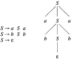
A simple e x a m p l e is the set of parse trees such as the one in Figure 1, for a g r a m m a r of palindromes. It is intuitively clear that the l a n g u a g e is not regular: the g r a m m a r symbols to the left of the spine f r o m the root to E " c o m m u n i c a t e " w i t h those to the right of the spine. More precisely, the prefix of the i n p u t u p to the p o i n t w h e r e it meets the final n o d e c of the spine d e t e r m i n e s the suffix after that point, in such a w a y that an u n b o u n d e d q u a n t i t y of symbols f r o m the prefix n e e d to be t a k e n into account.

(3)

Nederhof Experiments with Regular Approximation

S--',a S a S-->b S b S---~ ~

S

a S a

Y \

b S b

Figure 1

Grammar of palindromes, and a parse tree.

Definition

A g r a m m a r is s e l f - e m b e d d i n g if there is some A E N such that A --+* c~Afl, for some a ¢ e a n d f l ¢ e .

If a g r a m m a r is not self-embedding, this m e a n s that w h e n a section of a spine in a p a r s e tree repeats itself, t h e n either n o g r a m m a r symbols occur to the left of that section of the spine, or n o g r a m m a r symbols occur to the right. This p r e v e n t s the " u n b o u n d e d c o m m u n i c a t i o n " b e t w e e n the t w o sides of the spine exemplified b y the p a l i n d r o m e grammar.

We n o w p r o v e that g r a m m a r s that are not s e l f - e m b e d d i n g generate regular languages. For an arbitrary grammar, w e define the set of r e e u r s i v e n o n t e r m i n a l s as:

B

N = {A E N I Ag]}

m

We d e t e r m i n e the partition N" of N consisting of subsets N1, N2 . . . . , Nk, for some k > 0, of m u t u a l l y recursive nonterminals:

H = { N 1 , N 2 . . . . , N k }

N I U N 2 U . . . U N k = N Vi[Ni 7L O] Vi, j[i • j =~ Ni N Nj = 0]

a n d for all A, B E N:

3i[A E Ni A B @ Nil - ~oQ, fll, O~2,fl2[a ---~* alBfll A B ---+* c¢2Afl2],

We n o w define the function recursive f r o m N" to the set {left, right, self, cyclic}. For l < i K k :

recursive(Ni) -- left, if ~LeftGenerating(Ni) = right, if LeftGenerating(Ni) -- self, if LeftGenerating(Ni) = cyclic, if -,LeftGenerating(Ni)

/x RightGenerating(Ni) /x ~RightGenerating(Ni) /x RightGenerating(Ni) /x ~RightGenerating( Ni )

w h e r e

[image:3.468.34.174.49.167.2]

(4)

When

recursive(Ni) = left, Ni

consists of only left-recursive nonterminals, which does not mean it cannot also contain right-recursive nonterminals, but in that case right recursion amounts to application of unit rules. When

recursive(Ni) = cyclic,

it is

only

such unit rules that take part in the recursion.

That

recursive(Ni) = self,

for some i, is a sufficient and necessary condition for the grammar to be self-embedding. Therefore, we have to prove that if

recursive(Ni) E

{left, right, cyclic},

for all i, then the grammar generates a regular language. Our proof

differs from an existing proof (Chomsky 1959a) in that it is fully constructive: Fig- ure 2 presents an algorithm for creating a finite automaton that accepts the language generated by the grammar.

The process is initiated at the start symbol, and from there the process descends the grammar in all ways until terminals are encountered, and then transitions are created labeled with those terminals. Descending the grammar is straightforward in the case of rules of which the left-hand side is not a recursive nonterminal: the subautomata found recursively for members in the right-hand side will be connected. In the case of recursive nonterminals, the process depends on whether the nonterminals in the corresponding set from H are mutually left-recursive or right-recursive; if they are both, which means they are cyclic, then either subprocess can be applied; in the code in Figure 2 cyclic and right-recursive subsets

Ni

are treated uni- formly.

We discuss the case in which the nonterminals are left-recursive. One new state is created for each nonterminal in the set. The transitions that are created for terminals and nonterminals not in

Ni

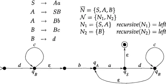
are connected in a w a y that is reminiscent of the construction of left-corner parsers (Rosenkrantz and Lewis 1970), and specifically of one construction that focuses on sets of mutually recursive nonterminals (Nederhof 1994, Section 5.8).

An example is given in Figure 3. Four states have been labeled according to the names they are given in procedure

make~fa.

There are two states that are labeled qB. This can be explained by the fact that nonterminal B can be reached by descending the grammar from S in two essentially distinct ways.

The code in Figure 2 differs from the actual implementation in that sometimes, for a nonterminal, a separate finite automaton is constructed, namely, for those nonterminals that occur as A in the code. A transition in such a subautomaton m a y be labeled by another nonterminal B, which then represents the subautomaton corresponding to B. The resulting representation is similar to extended context-free grammars (Purdom and Brown 1981), with the exception that in our case recursion cannot occur, by virtue of the construction.

The representation for the running example is indicated by Figure 4, which shows two subautomata, labeled S and B. The one labeled S is the automaton on the top level, and contains two transitions labeled B, which refer to the other subautomaton. Note that this representation is more compact than that of Figure 3, since the transitions that are involved in representing the sublanguage of strings generated by nonterminal B are included only once.

(5)

l e t K = O, A = O, s = fresh_state, f = fresh_state, F = { f } ;

make_fa( s, S, f ) .

p r o c e d u r e makeffa(qo, a, ql): i f a = e

t h e n l e t A = A U {(q0,e, ql)} e l s e i f a = a, s o m e a E ,U t h e n l e t A = A U {(q0, a, ql)}

e l s e i f a = Xfl, s o m e X E V, fl C V* s u c h t h a t IflI > 0 t h e n l e t q = fresh_state;

makeffa(qo, X , q);

makeffa( q, t , ql )

e l s e l e t A = a; (* a m u s t consist of a single n o n t e r m i n a l *) i f t h e r e e x i s t s i s u c h t h a t A C Ni

t h e n f o r e a c h B E Ni d o l e t qB = fresh_state e n d ; if recursive(Ni) = left

t h e n f o r e a c h ( C - + X I ' . ' X m ) E P s u c h t h a t C E N i A X 1 , . . . , X m ~ N i

d o make_fa(qo, X I " . X m , qc )

e n d ;

f o r e a c h (C --+ DX1 ... X,~) C P s u c h t h a t

C , D ~ Ni A X 1 , . . . , X m ~ Ni

d o make ffa( qD , X I " " X,~ , qc )

e n d ;

l e t A = A U {(qA, e, ql)}

e l s e (* recursive(g,) C {right, cyclic} *)

f o r e a c h ( C - + X 1 . . . X m ) E P s u c h t h a t C E N i A X 1 , . . . , X m ~ N i

d o make_fa(qc, X 1 . . .

Xm,

ql)

e n d ;

f o r e a c h (C --~ X I ".. X m D ) E P s u c h t h a t

C, D E Ni A X I , . . . , X m ~ Ni

d o makc_fa(qc, X I ".. X m ,

qD)

e n d ;

l e t A = A U {(qo, e, qa)}

e n d

e l s e f o r e a c h (A -+ fl) C P d o make_fa(qo,fl, ql) e n d (* A is n o t recursive *) e n d

e n d e n d .

p r o c e d u r e fresh_state():

create some o b j e c t q such t h a t q ~ K ; l e t K = K U { q } ;

r e t u r n q e n d .

Figure 2

(6)

S --* Aa

A --* SB

A ~ Bb

B --* Bc

B ---* d c

qB

Figure 3

N = { S , A , B }

]kf : {N1, N2}

N1 = {S,A} recursive(N1) = left N2 -- {B} recursive(N2) = left

__qA a d

Application of the code from Figure 2 on a small grammar. S

Figure 4

B

... 1

c

i i i I

, , . d ~ (~) ,

f w - w = i

qB I

The automaton from Figure 3 in a compact representation.

torial explosion that takes place u p o n n a i v e c o n s t r u c t i o n of a single n o n d e t e r m i n i s t i c finite a u t o m a t o n . 1

A s s u m e w e h a v e a list of s u b a u t o m a t a A1 . . . Am that is o r d e r e d f r o m lower-level to higher-level a u t o m a t a ; i.e., if a n a u t o m a t o n Ap occurs as the label of a transition of a u t o m a t o n Aq, t h e n p < q; Am m u s t be the start s y m b o l S. This o r d e r is a n a t u r a l result of the w a y that s u b a u t o m a t a are c o n s t r u c t e d d u r i n g o u r d e p t h - f i r s t t r a v e r s a l of the g r a m m a r , w h i c h is actually p o s t o r d e r in the sense that a s u b a u t o m a t o n is o u t p u t after all s u b a u t o m a t a o c c u r r i n g at its transitions h a v e b e e n o u t p u t .

O u r i m p l e m e n t a t i o n constructs a m i n i m a l d e t e r m i n i s t i c a u t o m a t o n b y r e p e a t i n g the following for p = 1 , . . . , m :

.

M a k e a c o p y of Ap. D e t e r m i n i z e a n d m i n i m i z e the copy. If it h a s f e w e r transitions labeled b y n o n t e r m i n a l s t h a n the original, t h e n replace Ap b y its copy.

Replace each transition in Ap of the f o r m (q, Ar, q') b y (a c o p y of)

a u t o m a t o n Ar in a s t r a i g h t f o r w a r d way. This m e a n s that n e w e-transitions c o n n e c t q to the start state of Ar a n d the final states of Ar t o qt.

[image:6.468.53.327.69.209.2] [image:6.468.50.364.71.342.2]

(7)

3. Again d e t e r m i n i z e a n d m i n i m i z e Ap a n d store it for later reference.

The a u t o m a t o n obtained for Am after step 3 is the desired result.

4. Methods of Regular Approximation

This section describes a n u m b e r of m e t h o d s for a p p r o x i m a t i n g a context-free gram- m a r b y m e a n s of a finite a u t o m a t o n . Some p u b l i s h e d m e t h o d s d i d not m e n t i o n self- e m b e d d i n g explicitly as the source of n o n r e g u l a r i t y for the language, a n d suggested that a p p r o x i m a t i o n s s h o u l d be applied globally for the complete grammar. W h e r e this is the case, w e a d a p t the m e t h o d so that it is m o r e selective a n d deals w i t h self-embedding locally.

The a p p r o x i m a t i o n s are integrated into the construction of the finite a u t o m a t o n from the grammar, w h i c h was described in the p r e v i o u s section. A separate incarnation of the a p p r o x i m a t i o n process is activated u p o n finding a n o n t e r m i n a l A such that A E Ni a n d recursive(Ni) = self, for some i. This incarnation t h e n o n l y pertains to the set of rules of the f o r m B --* c~, w h e r e B E Ni. In other w o r d s , n o n t e r m i n a l s not in Ni are treated b y this incarnation of the a p p r o x i m a t i o n process as if they w e r e terminals.

4.1 Superset Approximation Based on RTNs

The following a p p r o x i m a t i o n was p r o p o s e d in N e d e r h o f (1997). The p r e s e n t a t i o n here, however, differs substantially f r o m the earlier publication, w h i c h treated the ap- p r o x i m a t i o n process entirely on the level of context-free grammars: a s e l f - e m b e d d i n g g r a m m a r was t r a n s f o r m e d in such a w a y that it was n o longer self-embedding. A finite a u t o m a t o n was then obtained from the g r a m m a r b y the algorithm discussed above.

The presentation here is b a s e d on recursive transition n e t w o r k s (RTNs) (Woods 1970). We can see a context-free g r a m m a r as an RTN as follows: We introduce two states qA a n d q~ for each n o n t e r m i n a l A, a n d m + 1 states q0 . . . qm for each rule A --* X1 .. • Xm. T h e states for a rule A ~ X 1 . . . X m are c o n n e c t e d w i t h each other a n d

to the states for the left-hand side A b y one transition (qA, c, q0), a transition (qi-1, Xi, qi) for each i such that 1 < i < m, a n d one transition (qm, e,q~A). (Actually, some epsilon transitions are a v o i d e d in o u r i m p l e m e n t a t i o n , b u t w e will not be c o n c e r n e d w i t h such optimizations here.)

In this way, w e obtain a finite a u t o m a t o n with initial state qA a n d final state q~ for each n o n t e r m i n a l A a n d its defining rules A --* X1 • • • Xm. This a u t o m a t o n can be seen as one c o m p o n e n t of the RTN. The complete RTN is obtained b y the collection of all such finite a u t o m a t a for different nonterminals.

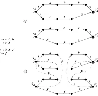
An a p p r o x i m a t i o n n o w results if w e join all the c o m p o n e n t s in one big a u t o m a t o n , and if w e a p p r o x i m a t e the usual m e c h a n i s m of recursion b y replacing each transition (q, A, q') b y t w o transitions (q, c, qA) a n d (q~, e, q'). The construction is illustrated in Figure 5.

(8)

(b)

a B b

(a)

d

A

e

qB Y ' ~

; i

=

i

~

'B

A---~ a B b

>t~

q

A---~c A

" ' " ~ " ~

f

B - - - ~ d A e

B--~ f

(c)

a b

~ ~ t /

Figure 5

Application of the RTN method for the grammar in (a). The RTN is given in (b), and (c) presents the approximating finite automaton. We assume A is the start symbol and therefore

qA

becomes the initial state and q~ becomes the final state in the approximating automaton.

For the sake of presentational convenience, the a b o v e describes a construction w o r k i n g o n the c o m p l e t e grammar. H o w e v e r , o u r i m p l e m e n t a t i o n applies the construction separately for each n o n t e r m i n a l in a set

Ni

such that

recursive(Ni) = self,

w h i c h leads to a separate s u b a u t o m a t o n of the c o m p a c t r e p r e s e n t a t i o n (Section 3).

See N e d e r h o f (1998) for a variant of this a p p r o x i m a t i o n that constructs finite trans- ducers rather t h a n finite automata.

We h a v e f u r t h e r i m p l e m e n t e d a p a r a m e t e r i z e d version of the RTN approximation. A state of the nondeterministic a u t o m a t o n is n o w also associated to a list H of length IHI strictly smaller than a n u m b e r d, w h i c h is the p a r a m e t e r to the m e t h o d . This list represents a history of rule positions that were e n c o u n t e r e d in the c o m p u t a t i o n leading to the present state.

M o r e precisely, w e define an i t e m to be an object of the f o r m [A ~ a • fl], w h e r e

A ~ aft

is a rule from the grammar. These are the same objects as the "dot- ted" p r o d u c t i o n s of Earley (1970). The dot indicates a position in the r i g h t - h a n d side.

[image:8.468.85.408.46.363.2]

(9)

H w i t h 0 < [HI < d that represents a series of positions in rules that c o u l d h a v e b e e n i n v o k e d before reaching I or A, respectively. More precisely, if w e set H = / 1 . . . In, t h e n each Im (1 < m < n) s h o u l d be of the f o r m [Am ~ olin • Bmflm] a n d for 1 < m < n w e s h o u l d h a v e Am -- Bm+l. F u r t h e r m o r e , for a state qiH w i t h I = [A --* a • fl] w e d e m a n d A = B1 if n > 0. For a state qAH w e d e m a n d A -- B1 if n > 0. (Strictly speaking, states qAH a n d qrH, w i t h [HI < d - 1 a n d I = [A --+ a • fl], will o n l y be n e e d e d if AIH ] is the start s y m b o l in the case IH[ > 0, or if A is the start s y m b o l in the case H = c.)

The transitions of the a u t o m a t o n that pertain to terminals in r i g h t - h a n d sides of rules are v e r y similar to those in the case of the u n p a r a m e t e r i z e d m e t h o d : For a state qIH with I of the f o r m [A ~ a • aft], w e create a transition (q~H, a, qi,H), w i t h I' = [A ~ aa • fl].

Similarly, w e create epsilon transitions that connect left-hand sides a n d r i g h t - h a n d sides of rules: For each state qAa there is a transition (qAH, e, qIH) for each item I = [A --* • a], for some a, a n d for each state of the f o r m qI,u, w i t h I' = [A ~ a •], there is a transition ( q F a , c, q~H).

For transitions that pertain to n o n t e r m i n a l s in the right-hand sides of rules, w e n e e d to m a n i p u l a t e the histories. For a state qIH w i t h I of the f o r m [A ~ a • Bfl], w e create t w o epsilon transitions. One is (qIH, c, qBn,), w h e r e H ' is defined to be I H if [IH[ < d, a n d to be the first d - 1 items of I H , otherwise. Informally, w e e x t e n d the history b y the item I representing the rule position that w e h a v e just c o m e from, b u t the oldest i n f o r m a t i o n in the history is discarded if the history b e c o m e s too long. The second transition is (q'BH,, ~, q~'H), w i t h I' = [A --* a B • fl].

If the start s y m b o l is S, the initial state is qs a n d the final state is q~ (after the s y m b o l S in the subscripts w e find e m p t y lists of items). N o t e that the p a r a m e t e r i z e d m e t h o d w i t h d -- 1 concurs w i t h the u n p a r a m e t e r i z e d m e t h o d , since the lists of items t h e n r e m a i n empty.

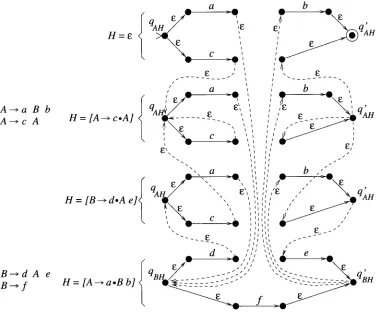
An e x a m p l e w i t h p a r a m e t e r d -- 2 is given in Figure 6. For the u n p a r a m e t e r i z e d m e t h o d , each I = [A --* a • fl] c o r r e s p o n d e d to one state (Figure 5). Since reaching A can h a v e three different histories of length shorter t h a n 2 (the e m p t y history, since A is the start symbol; the history of c o m i n g f r o m the rule position given b y item [A -~ c • A]; a n d the history of c o m i n g f r o m the rule position g i v e n b y item [B ~ d • Ae]), in Figure 6 w e n o w h a v e three states of the f o r m qI~ for each I -- [A ~ a • fl], as well as three states of the f o r m qA~r a n d q~H"

The h i g h e r w e choose d, the m o r e precise the a p p r o x i m a t i o n is, since the histories allow the a u t o m a t o n to simulate part of the m e c h a n i s m of recursion f r o m the original grammar, a n d the m a x i m u m length of the histories c o r r e s p o n d s to the n u m b e r of levels of recursion that can be simulated accurately.

4.2 Refinement of RTN Superset Approximation

We rephrase the m e t h o d of Grimley-Evans (1997) as follows: First, w e construct the a p p r o x i m a t i n g finite a u t o m a t o n according to the u n p a r a m e t e r i z e d RTN m e t h o d above. T h e n an additional m e c h a n i s m is i n t r o d u c e d that ensures for each rule A --~ X1 • .. Xm separately that the list of visits to the states q o , . . • • qm satisfies some reasonable criteria: a visit to qi, with 0 < i < m, s h o u l d be followed b y one to qi+l or q0. The latter option a m o u n t s to a n e s t e d incarnation of the rule. There is a c o m p l e m e n t a r y condition for w h a t s h o u l d p r e c e d e a visit to qi, w i t h 0 < i < m.

(10)

A ~ a B b

A ~ c A

B---,'d A e

B--->f

Figure 6

a

c

/

a

H = [A----> c . A l q A ~ _ . . . g ~',

x _, _a I I _,,

H = [B-->d.A el qA e',,

b

, E

b

i ,

, ,, .. ..

b "

,,'"

\ - q A .

d " ,,, , Z e _

qB Q~___

H = [A --~ a . B b] - - 5 . . "'L qBH

Application of the parameterized RTN method with d = 2. We again assume A is the start symbol. States qm have not been labeled in order to avoid cluttering the picture.

f i r m e d b y o u r o w n experiments, the n o n d e t e r m i n i s t i c finite a u t o m a t a resulting f r o m this m e t h o d m a y be quite large, e v e n for small g r a m m a r s . The e x p l a n a t i o n is that the n u m b e r of such histories is exponential in the n u m b e r of rules.

We h a v e refined the m e t h o d w i t h respect to the original publication b y a p p l y i n g the construction separately for each n o n t e r m i n a l in a set Ni such that recursive(Ni) = self.

4.3 Subset Approximation b y Transforming the Grammar

Putting restrictions on spines is a n o t h e r w a y to obtain a regular language. Several m e t h o d s can be defined. The first m e t h o d w e p r e s e n t investigates spines in a v e r y detailed way. It eliminates f r o m the l a n g u a g e o n l y those sentences for w h i c h a sub- d e r i v a t i o n is required of the f o r m B --~* aBfl, for some a ~ ¢ a n d fl ~ e. The m o t i v a t i o n is that such sentences do not occur f r e q u e n t l y in practice, since these s u b d e r i v a t i o n s m a k e t h e m difficult for p e o p l e to c o m p r e h e n d (Resnik 1992). Their exclusion will therefore not lead to m u c h loss of coverage of typical sentences, especially for simple application domains.

[image:10.468.50.426.51.363.2]

(11)

We are given a g r a m m a r G = (E,N, P, S). The following is to be p e r f o r m e d for each set Ni E A f such that recursive(Ni) = self.

. For each A E Ni a n d each F E 2 (Nix2~l''}), a d d the following nonterminal to N.

• A F .

2. For each A E Ni, a d d the following rule to P. • A---~A 0.

. For each (A --* o~0A1o~1A2... C~m-lAmCrm) E P such that A, A1 . . . . ,Am E Ni and no symbols from c~0 .. . . , am are members of Ni, a n d each F such that (A, (l, r}) ~ F, a d d the following rule to P.

a F _{o~0A 1 o q . . . A m O~m,}F1 Fm _{where, for 1 G j _< m,}

- - F j = {(B, Q U C ~ U ~ F ) I (B,Q) E F'};

F' = F U {(A, 0)} if -~3Q[(A,Q) E F], a n d F' = F otherwise;

- - • = 0 if c~0AlC~l...Aj-I~j-1 = c, a n d ~ = {l} otherwise; - - QJr = 0 if o/.jaj+lOLj+l...AmOL m = £ , a n d QJr = {r}

otherwise.

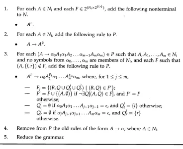
[image:11.468.38.406.86.387.2]

4. Remove from P the old rules of the form A --* c~, where A E Ni. 5. Reduce the grammar.

Figure 7

Subset approximation by transforming the grammar.

was generated. Similarly, r E Q indicates that something to the right was generated. If Q = {l, r}, then we have obtained a derivation B --** c~Afl, for some c~ ~ c a n d fl ~ ~, a n d further occurrences of B below A should be blocked in order to avoid a derivation w i t h self-embedding.

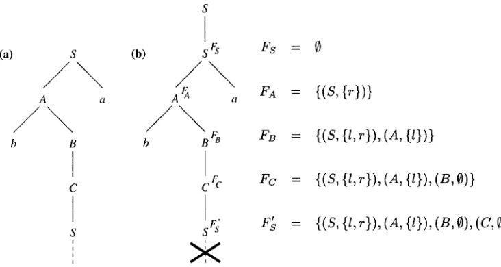
A n example is given in Figure 8. The original g r a m m a r is implicit in the depicted parse tree on the left, a n d contains at least the rules S --+ A a, A --, b B, B -* C, a n d C --* S. This g r a m m a r is self-embedding, since w e have a subderivation S --~* bSa. We explain h o w FB is obtained from FA in the rule A ~ --* b B r'. We first construct F' = {(S, {r}), (A, 0)} from FA = {(S, (r})} b y a d d i n g (A, 0), since no other pair of the form (A, Q) was already present. To the left of the occurrence of B in the original rule A --* b B we find a n o n e m p t y string b. This m e a n s that we have to a d d l to all second components of pairs in F', which gives us FB = {(S, (l, r}), (A, {l})}.

(12)

s

(a) s (b) s Fs F s =

A a a

/ \

FB

b B b B 'B

I

C ~ F c F c =

5 ' ' - -

s

X

0

{(S, {l, r}), (A, {/})}

{(S, {l, r}), (A, {/}), (B, 0)}

{(S, {l, r}), (A, {/}), (B, 0), (C, 0)}

Figure 8

A parse tree m a self-embedding grammar (a), and the corresponding parse tree in the transformed grammar (b), for the transformation from Figure 7. For the moment we ignore step 5 of Figure 7, i.e., reduction of the transformed grammar.

offending subderivation S --** c~Sfl has been found, further completion of the parse tree is blocked: the transformed g r a m m a r will n o t have a n y rules w i t h left-hand side

S {(S'{I'r})'(A'{I})'(B'O)'(C'O)}.

In fact, after the g r a m m a r is reduced, a n y parse tree that is

constructed can no longer even contain a n o d e labeled b y S {(s'U'r})'(a'{O)'(B'°)'(c'°)}, or a n y nodes w i t h labels of the form A r such that (A, {l,r}) c F.

One could generalize this approximation in such a w a y that not all self-embedding is blocked, b u t only self-embedding occurring, say, twice in a row, in the sense of a subderivation of the form A --** a l A f l l --+* oqol2Afl2fll. We will not do so here, because already for the basic case above, the transformed g r a m m a r can be h u g e d u e to the high n u m b e r of nonterminals of the form A F that m a y result; the n u m b e r of such nonterminals is exponential in the size of Ni.

We therefore present, in Figure 9, an alternative approximation that has a lower complexity. By parameter d, it restricts the n u m b e r of rules along a spine that m a y generate something to the left a n d to the right. We do not, however, restrict pure left recursion a n d pure right recursion. Between t w o occurrences of an arbitrary rule, we allow left recursion followed b y right recursion (which leads to tag r followed b y tag rl), or right recursion followed b y left recursion (which leads to tag l followed b y tag lr).

[image:12.468.50.416.54.249.2]

(13)

We are given a g r a m m a r G = (G, N, P, S). The following is to be p e r f o r m e d for each set Ni C .IV" such that recursive(Ni) = self. T h e v a l u e d stands for the m a x i m u m n u m b e r of u n c o n s t r a i n e d rules along a spine, possibly alternated w i t h a series of left-recursive rules followed b y a series of right-recursive rules, or vice versa.

1. For each A c Ni, each Q E { T, l, r, It, rl, 3_ }, a n d each f such that 0 < f < d, a d d the following n o n t e r m i n a l s to N.

• AQ,f.

2. For each A E Ni, a d d the following rule to P.

• A ---+ A T'0.

3. For each A E Ni a n d f such that 0 G f G d, a d d the following rules to P. • A T , f ___+ Al,f.

• ATd: __+ Ar,f.

• A i d ---+ Alr,f. • Ar,f ---, A~l,/.

• Atr,f __+ A ± , d .

• Arl,f ___+ A ± , f .

4. For each (A -+ Ba) ~ P such that A , B c Ni a n d no symbols f r o m ~ are m e m b e r s of Ni, e a c h f such that 0 < f G d, a n d each Q E {r, lr}, a d d the following rule to P.

• AQd ~ BQ/a.

5. For each (A --+ c~B) E P such that A , B E Ni and no symbols f r o m c~ are m e m b e r s of Ni, e a c h f such that 0 G f < d, a n d each Q c {l, rl}, a d d the following rule to P.

• A q d ~ c~BQ,f.

6. For each (A -~ o~0AloqA2... O~m-lAmC~m) C P such that A, A1 . . . Am E Ni a n d n o symbols from s0 . . . C~m are m e m b e r s of Ni, a n d each f such that 0 < f G d, a d d the following rule to P, p r o v i d e d m = 0 v f < d.

• A ± / - - - 4 c~0Alq-d+lc~l AT,f+1 . . . ~ l m ' O L m .

7. R e m o v e from P the old rules of the f o r m A ~ c~, w h e r e A E Ni. 8. R e d u c e the grammar.

Figure 9

A simpler subset approximation by transforming the grammar.

(14)

S

S !T,O

(a) / ~

(b)!r,O

So\

A a ' a

rl, O

b B b B rl'O

:o

t t

[image:14.468.52.244.49.288.2]

t t

Figure

10

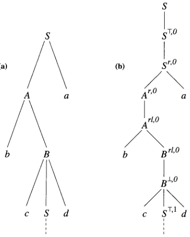
A parse tree in a self-embedding grammar (a), and the corresponding parse tree in the transformed grammar (b), for the simple subset approximation from Figure 9.

Figure 10 (b) is no longer possible, since no nonterminal in the transformed grammar would contain 1 in its superscript.

Because of the demonstrated increase of the counter f , this transformation is guar- anteed to remove self-embedding from the grammar. However, it is not as selective as the transformation we saw before, in the sense that it m a y also block subderivations that are not of the form A --** ~Afl. Consider for example the subderivation from Figure 10, but replacing the lower occurrence of S by any other nonterminal C that is mutually recursive with S, A, and B. Such a subderivation S ---** b c C d a would also be blocked by choosing d = 0. In general, increasing d allows more of such derivations that are not of the form A ~ " o~Afl but also allows more derivations that are of that form.

The reason for considering this transformation rather than any other that eliminates self-embedding is purely pragmatic: of the m a n y variants we have tried that yield nontrivial subset approximations, this transformation has the lowest complexity in terms of the sizes of intermediate structures and of the resulting finite automata.

In the actual implementation, we have integrated the grammar transformation and the construction of the finite automaton, which avoids reanalysis of the grammar to determine the partition of mutually recursive nonterminals after transformation. This integration makes use, for example, of the fact that for fixed Ni and fixed f , the set of nonterminals of the form A , f , with A c Ni, is (potentially) mutually right-recursive. A set of such nonterminals can therefore be treated as the corresponding case from Figure 2, assuming the value right.

(15)

4.4 Superset Approximation through Pushdown Automata

The distinction between context-free languages and regular languages can be seen in terms of the distinction between p u s h d o w n automata and finite automata. Pushdown automata maintain a stack that is potentially unbounded in height, which allows more complex languages to be recognized than in the case of finite automata. Regular approximation can be achieved by restricting the height of the stack, as we will see in Section 4.5, or by ignoring the distinction between several stacks when they become too high.

More specifically, the method proposed by Pereira and Wright (1997) first constructs an LR automaton, which is a special case of a p u s h d o w n automaton. Then, stacks that m a y be constructed in the course of recognition of a string are computed one by one. However, stacks that contain two occurrences of a stack symbol are iden- tified with the shorter stack that results by removing the part of the stack between the two occurrences, including one of the two occurrences. This process defines a congruence relation on stacks, with a finite number of congruence classes. This congruence relation directly defines a finite automaton: each class is translated to a unique state of the nondeterministic finite automaton, shift actions are translated to transitions labeled with terminals, and reduce actions are translated to epsilon transitions.

The method has a high complexity. First, construction of an LR automaton, of which the size is exponential in the size of the grammar, m a y be a prohibitively ex- pensive task (Nederhof and Satta 1996). This is, however, only a fraction of the effort needed to compute the congruence classes, of which the number is in turn exponential in the size of the LR automaton. If the resulting nondeterministic automaton is determinized, we obtain a third source of exponential behavior. The time and space complexity of the method are thereby bounded by a triple exponential function in the size of the grammar. This theoretical analysis seems to be in keeping with the high costs of applying this method in practice, as will be shown later in this article.

As proposed by Pereira and Wright (1997), our implementation applies the approximation separately for each nonterminal occurring in a set

Ni

that reveals self- embedding.

A different superset approximation based on LR automata was proposed by Baker (1981) and rediscovered by Heckert (1994). Each individual stack symbol is now translated to one state of the nondeterministic finite automaton. It can be argued theoret- ically that this approximation differs from the unparameterized RTN approximation from Section 4.1 only under certain conditions that are not likely to occur very often in practice. This consideration is confirmed by our experiments to be discussed later. Our implementation differs from the original algorithm in that the approximation is applied separately for each nonterminal in a set

Ni

that reveals self-embedding.

A generalization of this method was suggested by Bermudez and Schimpf (1990). For a fixed number d > 0 we investigate sequences of d top-most elements of stacks that m a y arise in the LR automaton, and we translate these to states of the finite automaton. More precisely, we define another congruence relation on stacks, such that we have one congruence class for each sequence of d stack symbols and this class contains all stacks that have that sequence as d top-most elements; we have a separate class for each stack that contains fewer than d elements. As before, each congruence class is translated to one state of the nondeterministic finite automaton. Note that the case d = 1 is equivalent to the approximation in Baker (1981).

(16)

4.5 Subset Approximation through Pushdown Automata

By restricting the height of the stack of a p u s h d o w n automaton, one obstructs recognition of a set of strings in the context-free language, a n d therefore a subset approximation results. This idea was proposed b y K r a u w e r a n d des Tombe (1981), L a n g e n d o e n a n d Langsam (1987), a n d P u l m a n (1986), a n d was rediscovered b y Black (1989) a n d recently b y Johnson (1998). Since the latest publication in this area is more explicit in its presentation, we will base our treatment on this, instead of going to the historical roots of the method.

One first constructs a modified left-corner recognizer from the grammar, in the form of a p u s h d o w n automaton. The stack height is b o u n d e d b y a low number; Johnson (1998) claims a suitable n u m b e r w o u l d be 5. The motivation for using the left-corner strategy is that the height of the stack m a i n t a i n e d b y a left-corner parser is already b o u n d e d b y a constant in the absence of self-embedding. If the artificial b o u n d i m p o s e d b y the approximation m e t h o d is chosen to be larger t h a n or equal to this natural b o u n d , then the approximation m a y be exact.

Our o w n i m p l e m e n t a t i o n is more refined t h a n the published algorithms m e n t i o n e d above, in that it defines a separate left-corner recognizer for each nonterminal A such that A E Ni a n d recursive(Ni) = self, some i. In the construction of one such recognizer, nonterminals that do not belong to Ni are treated as terminals, as in all other m e t h o d s discussed here.

4.6 Superset Approximation by N-grams

A n approximation from Seyfarth a n d Bermudez (1995) can be explained as follows. Define the set of all terminals reachable from nonterminal A to be ~A = {a I 3c~, iliA --** o~afl]}. We n o w approximate the set of strings derivable from A b y G~, w h i c h is the set of strings consisting of terminals from GA. Our i m p l e m e n t a t i o n is m a d e slightly more sophisticated b y taking ~A to be {X ] 3B, c~,fl[B E Ni A B ~ oLXfl A X ~

Ni]},

for each A such that A E Ni a n d recursive(Ni) = self, for some i. That is, each X E ~A is a terminal, or a nonterminal not in the same set Ni as A, b u t i m m e d i a t e l y reachable from set Ni, t h r o u g h B E Ni.

This m e t h o d can be generalized, inspired b y Stolcke a n d Segal (1994), w h o derive N-gram probabilities from stochastic context-free grammars. By ignoring the probabilities, each N = 1, 2, 3 . . . . gives rise to a superset approximation that can be described as follows: The set of strings derivable from a nonterminal A is approximated b y the set of strings al . . . an such that

• for each substring v = ai+l . . . ai+N (0 < i < n -- N ) w e have A --+* w v y , for some w a n d y,

• for each prefix v = al . . . ai (0 < i < n) such that i < N w e have A -** vy, for some y, a n d

• for each suffix v = ai+l . . . an (0 < i < n) such that n - i < N w e have a ---~* wv, for some w.

(Again, the algorithms that w e actually i m p l e m e n t e d are more refined a n d take into account the sets Ni.)

(17)

5. Increasing the Precision

The methods of approximation described above take as input the parts of the grammar that pertain to self-embedding. It is only for those parts that the language is affected. This leads us to a w a y to increase the precision: before applying any of the above methods of regular approximation, we first transform the grammar.

This grammar transformation copies grammar rules containing recursive nonterminals and, in the copies, it replaces these nonterminals b y new nonrecursive nonterminals. The new rules take over part of the roles of the old rules, but since the new rules do not contain recursion and therefore do not pertain to self-embedding, they remain unaffected by the approximation process.

Consider for example the palindrome grammar from Figure 1. The RTN method will yield a rather crude approximation, namely, the language {a, b}*. We transform this grammar in order to keep the approximation process away from the first three levels of recursion. We achieve this by introducing three new nonterminals S[1], S[2] and S[3], and by adding modified copies of the original grammar rules, so that we obtain:

S[1] S[2] S[3] S

The new start symbol is S[1].

a S [ 2 ] a ] bS[2] b I ¢ a S [ 3 ] a ] bS[3] b I c

a S a l b S b i c a S a i b S b i e

The new grammar generates the same language as before, but the approximation process leaves unaffected the nonterminals S[1], S[2], and S[3] and the rules defining them, since these nonterminals are not recursive. These nonterminals amount to the upper three levels of the parse trees, and therefore the effect of the approximation on the language is limited to lower levels. If we apply the RTN method then we obtain the language that consists of (grammatical) palindromes of the form ww R, where

w E {¢, a, b} U {a, b} 2 U {a, b} 3, plus (possibly ungrammatical) strings of the form w v w R,

where w E {a, b} 3 and v E {a, b}*. (w R indicates the mirror image of w.)

The grammar transformation in its full generality is given by the following, which is to be applied for fixed integer j > 0, which is a parameter of the transformation,

and for each Ni such that recursive(Ni) = self.

For each nonterminal A E Ni we introduce j new nonterminals All] . . . A~]. For

each A --, X 1 . . . X m in P such that A E Ni, and h such that 1 ~ h < j, we add

A[h] --* X ' I . . . X " to P, where for 1 < k < m:

X~k = Xk[h + 1] if X k E Ni /X h < j

= Xk otherwise

Further, we replace all rules A --* X1 . . . Xm such that A ~ Ni by A --* X~ ... X~m, where for 1 < k < m:

X~ -- Xk[1] i f X k E N i

= Xk otherwise

If the start symbol S was in Ni, we let S[1] be the new start symbol.

(18)

550 500 450

• 400

-5 350 ._N_ 300 250

E 200 E

150 100 50 0 0

I I I I I I

50 100 150 200 250 300 350

corpus size (# sentences)

E 180

160

140

120

100

80

60

40

20

0

5 10 15 20 25 30

length (# words)

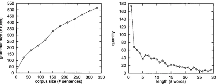
Figure 11

The test material. The left-hand curve refers to the construction of the grammar from 332 sentences, the right-hand curve refers to the corpus of 1,000 sentences used as input to the finite automata.

6. Empirical Results

In this section we investigate empirically how the respective approximation methods behave on grammars of different sizes and how much the approximated languages differ from the original context-free languages. This last question is difficult to answer precisely. Both an original context-free language and an approximating regular language generally consist of an infinite number of strings, and the number of strings that are introduced in a superset approximation or that are excluded in a subset approximation m a y also be infinite. This makes it difficult to attach numbers to the "quality" of approximations.

We have opted for a pragmatic approach, which does not require investigation of the entire infinite languages of the grammar and the finite automata, but looks at a certain finite set of strings taken from a corpus, as discussed below. For this finite set of strings, we measure the percentage that overlaps with the investigated languages.

For the experiments, we took context-free grammars for German, generated automatically from an HPSG and a spoken-language corpus of 332 sentences. This corpus consists of sentences possessing grammatical phenomena of interest, manually selected from a larger corpus of actual dialogues. An HPSG parser was applied on these sentences, and a form of context-free backbone was selected from the first derivation that was found. (To take the first derivation is as good as any other strategy, given that we have at present no mechanisms for relative ranking of derivations.) The label occurring at a node together with the sequence of labels at the daughter nodes was then taken to be a context-free rule. The collection of such rules for the complete corpus forms a context-free grammar. Due to the incremental nature of this construction of the grammar, we can consider the subgrammars obtained after processing the first p sentences, where p = 1, 2, 3 . . . 332. See Figure 11 (left) for the relation between p and the number of rules of the grammar. The construction is such that rules have at most two members in the right-hand side.

[image:18.468.54.423.52.195.2]

(19)

51 and 60 words. In most cases however such long strings are in fact composed of a number of shorter sentences.

Each of the 1,000 sentences were input in their entirety to the automata, although in practical spoken-language systems, often one is not interested in the grammaticality of complete utterances, but tries to find substrings that form certain phrases bearing information relevant to the understanding of the utterance. We will not be concerned here with the exact way such recognition of substrings could be realized by means of finite automata, since this is outside the scope of this paper.

For the respective methods of approximation, we measured the size of the compact representation of the nondeterministic automaton, the number of states and the number of transitions of the minimal deterministic automaton, and the percentage of sentences that were recognized, in comparison to the percentage of grammatical sentences. For the compact representation, we counted the number of lines, which is roughly the sum of the numbers of transitions from all subautomata, not considering about three additional lines per subautomaton for overhead.

We investigated the size of the compact representation because it is reasonably implementation independent, barring optimizations of the approximation algorithms themselves that affect the sizes of the subautomata. For some methods, we show that there is a sharp increase in the size of the compact representation for a small increase in the size of the grammar, which gives us a strong indication of how difficult it would be to apply the method to much larger grammars. Note that the size of the compact representation is a (very) rough indication of how much effort is involved in determinization, minimization, and substitution of the subautomata into each other. For determinization and minimization of automata, we have applied programs from the FSM library described in Mohri, Pereira, and Riley (1998). This library is considered to be competitive with respect to other tools for processing of finite-state machines. When these programs cannot determinize or minimize in reasonable time and space some subautomata constructed by a particular method of approximation, then this can be regarded as an indication of the impracticality of the method.

We were not able to compute the compact representation for all the methods and all the grammars. The refined RTN approximation from Section 4.2 proved to be quite problematic. We were not able to compute the compact representation for any of the automatically obtained grammars in our collection that were self-embedding. We therefore eliminated individual rules by hand, starting from the smallest self- embedding grammar in our collection, eventually finding grammars small enough to be handled by this method. The results are given in Table 1. Note that the size of the compact representation increases significantly for each additional grammar rule. The sizes of the finite automata, after determinization and minimization, remain relatively small.

(20)

Table 1

Size of the compact representation and number of states and transitions, for the refined RTN approximation (Grimley-Evans 1997).

Grammar Size Compact Representation # of States # of Transitions

10 133 11 14

12 427 17 26

13 1,139 17 34

14 4,895 17 36

15 16,297 17 40

16 51,493 19 52

17 208,350 19 52

18 409,348 21 59

19 1,326,256 21 61

Table 2

Size of the compact representation and number of states and transitions, for the superset approximation based on LR automata following Pereira and Wright (1997).

Grammar Size Compact Representation # of States # of Transitions

35 15,921 350 2,125

44 24,651 499 4,352

47 151,226 5,112 35,754

50 646,419 ? ?

Below, w e refer to the u n p a r a m e t e r i z e d a n d p a r a m e t e r i z e d a p p r o x i m a t i o n s b a s e d o n RTNs (Section 4.1) as RTN a n d RTNd, respectively, for d = 2,3; to the subset a p p r o x i m a t i o n f r o m Figure 9 as Subd, for d = 1, 2, 3; a n d to the second a n d third m e t h o d s f r o m Section 4.4, w h i c h w e r e b a s e d o n LR p a r s i n g following Baker (1981) a n d B e r m u d e z a n d Schimpf (1990), as LR a n d LRd, respectively, for d = 2, 3. We refer to the subset a p p r o x i m a t i o n b a s e d o n left-corner p a r s i n g from Section 4.5 as LCd, for the m a x i m a l stack height of d = 2, 3, 4; a n d to the m e t h o d s discussed in Section 4.6 as Unigram, Bigram, a n d Trigram.

We first discuss the c o m p a c t r e p r e s e n t a t i o n of the n o n d e t e r m i n i s t i c automata. In Figure 12 w e use t w o different scales to be able to represent the large v a r i e t y of values. For the m e t h o d Subd, the c o m p a c t r e p r e s e n t a t i o n is of p u r e l y theoretical interest for g r a m m a r s larger t h a n 156 rules in the case of Sub1, for those larger t h a n 62 rules in the case of Sub2, a n d for those larger t h a n 35 rules in the case of Sub3, since the minimal deterministic a u t o m a t a c o u l d thereafter n o longer be c o m p u t e d w i t h a reasonable b o u n d o n resources; w e s t o p p e d the processes after t h e y h a d c o n s u m e d o v e r 400 megabytes. For LC3, LC4, RTN3, LR2, a n d LR3, this was also the case for g r a m m a r s larger t h a n 139, 62, 156, 217, a n d 156 rules, respectively. The sizes of the c o m p a c t representation seem to g r o w m o d e r a t e l y for LR a n d Bigram, in the u p p e r panel, yet the sizes are m u c h larger t h a n those for RTN a n d U n i g r a m , w h i c h are indicated in the l o w e r panel.

[image:20.468.52.356.98.224.2] [image:20.468.48.359.281.346.2]

(21)

Nederhof Experiments with Regular Approximation

r'~

E

O o

7 0 0 0 0 0

6 0 0 0 0 0

5 0 0 0 0 0

4 0 0 0 0 0

3 0 0 0 0 0

2 0 0 0 0 0

1 0 0 0 0 0

0

i i ] ; ; / i i

, / ! /' LC4

! / / ," LR3--x---.

i [ / ., R T N 3 - ~

i I i ," L C 3

i [ i " LR2 . . .

! / j Trigram -~'---

, / ; LC2 -e---

i / i R T N 2

i / / LR - + --

:t ] / Bigram-E3---

~: ~ ;'

~ /'

! /" / / 4-

/ ," ,4- ... + ....

" / ' / ' ~ 4-"""

,' / . - " _..+ ... 4- ...

' ~-~ "" - - - - E 3 - . . . E } . . . E } - - - - n . . . . - - ' -

- - . . . 1 . . . I I I I I I

50 100 1 5 0 2 0 0 2 5 0 3 0 0 3 5 0 4 0 0 4 5 0 5 0 0 5 5 0 g r a m m a r size

2 0 0 0 0

1 5 0 0 0

"3

&

1 0 0 0 0

o

5 0 0 0

IJ

:/

/" / /" / /.' ,.'

,; ,.: ,"

i ... ,'

,,..,' ...." ,,,'

/

,,: ,,, ..,..

.: ....

z ~ ,'" . .. " ~ /

... ,' . ...' .-

...- ,,• y~..- " ' " " ' ' , , , ~ ::'~ ...

0 50 1 0 0 1 5 0 2 0 0

Figure 12

Size of the compact representation.

R T N 2 .-a-- L C 2 - e - - LR - + --' Bigram -~--- S u b 3 -x . . . .

S u b 2 "a ... Sub1 -~ ...

R T N Unigram -~,---

....

.,0.

I I I I I I

2 5 0 3 0 0 3 5 0 4 0 0 4 5 0 5 0 0 5 5 0 g r a m m a r size

[image:21.468.35.387.50.589.2]

(22)

1 0 0 0 0

9 0 0 0

8 0 0 0

7 0 0 0

6 0 0 0

5 0 0 0

4000

3 0 0 0

2000

1000

0

Sub2 ..A ... L C 4 - 8 - - Sub1 --~ ... L C 3 - x - - R T N 3

L C 2 - e - -

f

/

j

/

[ / /

~ ~ ~ i

100

° ~ - ' ~ - ~ ~

0 2 0 0 3 0 0 4 0 0 5 0 0 6 0 0

g r a m m a r size

100 , , , , ,

L C 3 R T N 3

L R 3 --x- -- L C 2 - e - -

x R T N 2

8 0 ,,,,,," TrigramLR2 -.~--~----

LR - + -- RTN - B ~ Bigram -a--

~ - - ~ - Unigram -~---

60 .~¢"

/

40

: ~ ~ d~3._-.D . D - - - [ ] ' - - - • . . . ~E]" * . . . [ ] . . . -

2 0 " ~" --e-- "<>

. . e - . . . e . . . -e . . . ~ . . .

0 i i i i i

0 100 2 0 0 3 0 0 4 0 0 5 0 0 6 0 0

[image:22.468.51.397.56.579.2]

g r a m m a r size

Figure 13

Number of states of the deterrninized and m i n i m i z e d automata.

(23)

(Figure 12) are much larger. It should therefore be concluded that the "sophistication" of LR parsing is here merely an avoidable source of inefficiency.

The numbers of transitions for the respective methods are given in Figure 14. Again, note the different scales used in the two panels. The numbers of transitions roughly correspond to the storage requirements for the automata. It can be seen that, again, Trigram, LR, RTN, Bigram, and Unigram perform well.

The precision of the respective approximations is measured in terms of the percentage of sentences in the corpus that are recognized b y the automata, in comparison to the percentage of sentences that are generated b y the grammar, as presented by Fig- ure 15. The lower panel represents an enlargement of a section from the upper panel. Methods that could only be applied for the smaller grammars are only presented in the lower panel; LC4 and Sub2 have been omitted entirely.

The curve labeled G represents the percentage of sentences generated by the grammar. Note that since all approximation methods compute either supersets or subsets, a particular automaton cannot both recognize some ungrammatical sentences and reject some grammatical sentences.

Unigram and Bigram recognize very high percentages of ungrammatical sentences. Much better results were obtained for RTN. The curve for LR would not be distin- guishable from that for RTN in the figure, and is therefore omitted. (For only two of the investigated grammars was there any difference, the largest difference occurring for grammar size 217, where 34.1 versus 34.5 percent of sentences were recognized in the cases of LR and RTN, respectively.) Trigram remains very close to RTN (and LR); for some grammars a lower percentage is recognized, for others a higher percentage is recognized. LR2 seems to improve slightly over RTN and Trigram, but data is available only for small grammars, due to the difficulty of applying the method to larger grammars. A more substantial improvement is found for RTN2. Even smaller percentages are recognized by LR3 and RTN3, but again, data is available only for small grammars.

The subset approximations LC3 and Sub1 remain very close to G, but here again only data for small grammars is available, since these two methods could not be applied on larger grammars. Although application of LC2 on larger grammars required relatively few resources, the approximation is very crude: only a small percentage of the grammatical sentences are recognized.

We also performed experiments with the grammar transformation from Section 5, in combination with the RTN method. We found that for increasing j, the intermediate automata soon became too large to be determinized and minimized, with a bound on the memory consumption of 400 megabytes. The sizes of the automata that we were able to compute are given in Figure 16. RTN+j, for j = 1, 2, 3,4, 5, represents the (unparameterized) RTN method in combination with the grammar transformation with parameter j. This is not to be confused with the parameterized RTNd method.

(24)

9 0 0 0 0

8 0 0 0 0

7 0 0 0 0

6 0 0 0 0

5 0 0 0 0 o

4 0 0 0 0

3 0 0 0 0

2 0 0 0 0 100OO 0

0

z~

100 2 0 0 3 0 0 4 0 0 5 0 0 g r a m m a r size

i

S u b 2 --~ ... L C 4 Sub1 --~ ...

L C 3 L C 2 R T N 2

I

6 0 0

5 0 0 0

4 0 0 0 -

0000 /

/!

'

2 0 0 0 - /

/ -

. / / ' / ' /';'"

. 1 3 - - - _ D - / ";Y" _ . . . ~ - . . . 43"-

1 0 0 0 I I .:..i~ ..- .... (3 . . . .

. D -''0

L C 3 - x - - - R T N 3

L R 3 --x- -- L C 2 - e ~ R T N 2 T r i g r a m -~---

L R 2 -~,- -- L R - ÷ -- R T N B i g r a m - B - - U n i g r a m -~- --

0 1 0 0 2 0 0 3 0 0 4 0 0 5 0 0

g r a m m a r size

Figure 14

Number of transitions of the determinized and minimized automata.

6 0 0

7. C o n c l u s i o n s

[image:24.468.47.395.44.589.2]

(25)

Nederhof Experiments with Regular Approximation

1 0 0 8 0 -o 6O

&

oo

4 0 0 0 2 0

Unigram -4- -- Bigram -[]-- , e - - - ~ Trigram -x--.- ,,' R T N ( L R ) - ~ - - e- . . . ¢, -- --e- -- -~- . . . '~ RTN2G -~---~a-- . . ' L C 2 - e - -

• 1 3 - * - £ 3 ,.O . . . ~" ~3 . . . (3" "'" 13 . . . E l - - - - [ ] ' - ' -

[ ] . . . Ey •

/ , - _ . l q _ _ _ +

/' ,' 4 . . - I

6 , ~ ' 0 0 . _ . - - - e - - ~ O 0

• C] / /

i" I I

1 0 0 2 0 0 3 0 0 4 0 0 5 0 0 6 0 0 g r a m m a r size

5'

,[::

4

"E