Real-Time Internet-Based Teleoperation
Ehsan Kamrani
Electrical Engineering Department, Ecole Polytechnique de Montreal, Montreal, Canada Email: [email protected]
Received July 2,2012; revised August 2, 2012; accepted August 9, 2012
ABSTRACT
Internet-based teleoperation employs robots and internet a two breakthrough technologies to manipulate robots from distance for different applications. Variable and unknown time delay dynamics of internet is the main obstacle for real- time teleoperation via internet. In this paper the internet delay dynamics and its characteristics have been studied based on the measurement in different nodes. Then a black-box model for end-to-end internet delay dynamics has been de- veloped using system identification and Auto-Regressive eXogeneous (ARX) model. Our experimental studies show a regular periodic behaviour in long-term intervals of internet delay variation and also confirm the accuracy and reliabil- ity of our theoretical and modelling derivations. This paper also introduces a novel multivariable control method for real-time telerobotic operations via Internet. Random communications delay of the Internet can cause instability in real- time closed-loop telerobotic systems. When a single identification model is used, it will have to adapt itself to the oper- ating condition before an appropriate control mechanism can be applied. Slow adaptation may result in a large transient error. As an alternative, we propose to use a Multiple Model framework. The control strategy is to determine the best model for the current operating condition and activate the corresponding controller. We propose the use of Multi-Model Adaptive Control Theory and Multivariable Wave prediction method to capture the concurrency and complexity of Internet-based teleoperation. The results confirm the efficiency of the proposed technique in dealing with constant and variable delay dynamics of internet.
Keywords: Teleoperation; Delay Dynamic; Internet; Modelling and Simulation; Wave Prediction; Robot Control
1. Introduction
Robotics and Internet industry can be considered as one of the most important specification of the technology improvement today. The concept of teleoperation has been around for awhile. It involves remote control of a plant or machine from far distance via a medium envi- ronment. Generally remote control of a plant or machine from far distance and via a medium environment is called teleoperation. The distance can vary from tens of centi- metres (micromanipulation) to millions of kilometres (space applications). Teleoperation takes several forms and can he done via any communication medium. Re- cently, the main focus has been on teleoperation via the Internet. Motivated by the availability, widespread access, and low cost of the Internet, many researchers have fo- cused on the Internet-based teleoperation. Since the Internet introduces random communication delays, sev- eral challenges and difficulties, such as loss of transpar- ency, and de-synchronization in real-time closed-loop telerobotic systems, may arise.
In order to meet these challenges, a general and effi- cient modeling and analysis tool for the Internet delay needs to be developed. Several techniques have been
proposed to compensate for this effect, such as time for- ward observer developed for a supervisory control over the Internet [1,2], position-based force-feedback [3], and wave variable based techniques [4].
Using independent of delay (IOD) technique [5], the stability achieves by degrading transparency especially while the delay increases. The methods which need the knowledge of the remote robot [2-6] are not applicable due to probability of the remote plan uncertainties. More- over their stability may be depended on the accuracy and reliability of the available information from remote plant. Anderson and Spong [6,7] proposed using wave-vari- ables for stable teleoperation in a time constant delay. The wave-based technique was more intuitively and phy- sically developed by Slotine [8] and later was extended for variable time-delay teleoperations [9-12].
measurement in different nodes and developed a realistic black-box model for internet delay dynamics associated with internet communication link using system identify- cation. This model then has been applied in a novel multi-model adaptive control platform in conjunction with wave-prediction and passivity technique.
As a consequence, in this paper the internet dynamics and its main parameters are introduced in Section 2. In Section 3 the internet delay dynamics are studied, meas- ured and modelled for control and telepperation applica- tions. The wave variable, smith predictor and nonlinear adaptive control techniques are introduced and imple- mented in Sections 4-6. A multi-model adaptive control system is also designed and implemented in Section 7 for stable real-time teleoperation with time varying internet dynamics.
2. Dynamics of the Internet
2.1. Description of Internet Based on Its QoS Parameters
Internet communication technology has changed our communicational practices and it is almost available everywhere with low cost. Using internet as a communi- cation link for remote operations will widely spreads the application of teleopeartion systems with highest acces- sibility, ease of use and low cost [2,20]. Remote envi- ronments limit access to power and telecommunication resources needed by telerobot systems. Mobile robots applied for teleoperation applications (e.g. telesurgery) most provide real-time access to the remote plans with a stable closed-loop control [21], regardless of their loca- tion, environment and internet delay dynamics [3]. However the variable and random dynamic behaviour of internet time-delay impedes transparent and real-time teleoperations over internet [4,22]. In order to overcome this limitation, a general and reliable model of the inter- net delay dynamics and a stable control system platform to manipulate teleoperator via this communication link are required.
It is very important to have a deeply understand the end-to-end internet delay dynamics as it directly affects on the quality of service (QoS) [23,24] in real-time ap- plications. It also enable design and develop an efficient teleoperation control system for both real-time and off- line applications. The queuing theory has been applied widely as a powerful tool to analyze both packet-switch- ed and circuit-switched networks. Nevertheless, due to its limitations, the queuing theory is not proper for network delay dynamics analysis. Several measurement-based studies imply that the end-to-end packet time delay in the Internet is quite dynamic [5-7] and many works also have been published describing the end-to-end packet time delay [8,9,25-27] and the end-to-end path specifications
[10,26].
In a study on end-to-end packet delay and packet loss in the Internet using small UDP probe packets [5], the correlation between the actual packet delay and the packet loss is examined. In [10], the routing behaviour of the Internet has been analyzed using measurements of about 40,000 end-to-end trace route results. The delay dynamics of the Internet have been analyzed in [7] based on measurements of about 20,000 TCP data transfers. The loss and delay characteristics of a transmission link are also presented using end-to-end multicast measure- ments in [9]. In [11], the Internet delay is measured and analyzed at 3 sample nodes in the Internet at random instances, but no description of the delay dynamics is provided. The above studies all are limited to the study of statistical behaviour of the end-to-end packet delays or path characteristics, however the end-to-end packet delay dynamics of the Internet, which are very critical for real- time stable teleoperation via internet have not been in- vestigated yet. Several measurement-based studies have also been applied for black-box modeling of the internet traffic [12-15]. In [12], a traffic model for wide-area TCP traffic has been proposed by characterizing several dis- tributions of different parameters, such as the number of transferred bytes and the packet inter-arrival time. A fast algorithm to construct a Circulant Modulated Rate Proc- ess (CMRP) for traffic modeling also has been offered in [13]. The CMRP and auto-regressive moving average (ARMA) have been used in [14] to model the internet traffic.
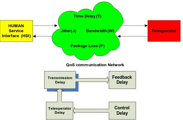
Here we have analyzed the internet delay dynamics based on the measurements and developed an ARX black-box model for internet delay dynamics. This model can be used, in particular, to design an efficient delay based teleoperation control system using the optimal control theory. The ARX model is simple, easy to handle, useful in the domain of control theory, and its coeffi- cients are easily determined with minor computations. The main parameters describing internet performance in terms of QoS [16] includes: time-delay, Jitter, Bandwidth and Packet-loss (Figure 1). To improve the performance, the time delays need to be minimized. The impact of other parameters can be reduced using existing methods, which usually involve a trade-off with the time delay. So, the QoS improvement in general involves minimization of the time delay, which is our main concern at this re- search work.
2.2. Time Delay
Time Delay (T)
Jitter(J) Bandwidth (W)
Package Loss (P)
Teleoperator
HUMAN Service Interface (HSI)
QoS communication Network
Transmission Delay
Feedback Delay
Teleoperator Delay
[image:3.595.154.446.84.276.2]Control Delay
Figure 1. Block diagram of teleoperation system in a QoS network and delay in teleoperation systems.
tion is show. This is because of the delay in the system. There is always delay in the remote operation system. And each part has some delay. The digital systems in- crease the delay in the remote operation system. Accord- ing to Shannon’s law, the measuring frequency should be move than two times of the highest frequency. In systems with long delay, the remote operation performs in a “move and wait” manner. When the delay applies to a signal accidentally, the signal become a module signal and the move delay for this frequency, the move similar- ity to a modulate signal. This modulate signal can cause instability in system.
Time delay defines as the average required time by a packet in the communication link to travel from the sender to the receiver. The internet time delay includes the queuing, processing and propagation delay inspired by switches, and communication links. The main QoS parameter is the time delay, because applying any tech- nique affecting on improvement of other parameters usu- ally involves a trade-off with delay. Furthermore to im- prove the performance, at the end the delay need to be minimized. So improvement of QoS in internet-based teleoperation in general involves minimization of the time delay. Applying any technique which decreases the time delay or its effects on the stability of the system will improve the whole system performance and efficiency.
2.3. Jitter
The random queuing delay in the communication link and network devices is an important part of the end-to- end time-delay. Due to these varying delays within the network, the travel time for a packet can vary from a packet to a packet. This phenomenon is called jitter. It is assumed that the end-to-end time delay is given by:
, with jitter J representing a maximum value of
deviation, represented in Figure 2(a).
In Figures 2(b) and (c), the master and slave position are shown, respectively with and without jitter for two different master signal frequencies. In general if the maximum jitter is smaller than half width of the strobe impulse of the digital-to-analog-converter (DAC), it will have no effect on the signal. However, usually it is great- er than that. The distortion caused by jitter introduces high frequency noise and possible destabilization in the system [18]. By employing reconstruction filters [19] the destabilizing effect of jitter can resolved [25-27]. Other applied techniques for jitter compensation includes: de- laying play-out, prefacing each chunk with a timestamp, and prefacing each chunk with a sequence number [16].
2.4. Band Width
The Bandwidth (BW) which also refers to as the net bit rate or channel capacity, defines the maximum data transmission rate in a communication link. It specifies the maximum throughput of the physical communication path. Internet bandwidth can be thought of as an elec- tronic byway that connects the Internet to the computer. Increasing bandwidth allows more traffic to flow, in- creasing speed. For teleoperation systems, the BW de- pends on the applied protocol and also the resolution and sampling rate of the force and position signals. Teleop- eration is BW-sensitive [3], so the required BW for data transmission including the protocol overhead should be reduced. In UDP, the protocol overhead is smaller com- paring to TCP and also using UDP, a consistent sample rate can be gained with lower fluctuations [25-27].
2.5. Packet Loss
Packet loss or increasing time delay in teleoperation sys- tem may result in a buffer under-run at the receiver side 1
(a)
(b)
(c)
Figure 2. The slave position in response to the master signal (dash-dotted) with fixed delay (dashed-blue) and with jitter (solid-red) according to the delay shown in (c).
and destabilize the whole control system [28-30]. Usu- ally the packet loss is due to the over-loading of the net- work which causes dropping the packet by network de- vice. It depends on the applied queuing technique and load in the network node. Using UDP offers lower packet loss and is preferred [26,31,32]. However some tech- niques such as forward error correction (FEC) which
offers redundancy in sent packets are also applied for packet loss compensation [26].
3. Dynamics of Internet Time-Delay
3.1. Experimental Determination of Time Delay: Delay Dynamics in Real Internet
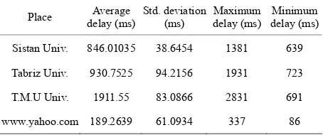
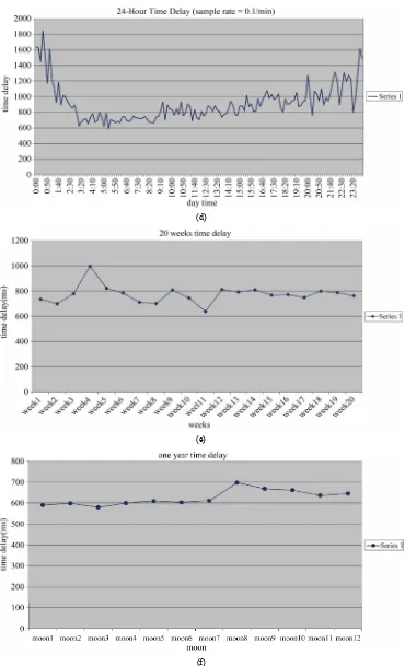
[image:4.595.58.288.87.602.2] [image:4.595.310.537.641.736.2]Experimental data were collected for the typical time delays encountered by the data packets between the host and the client. In these experiments the host PC and the client PC were connected to the different local area net- works (LANs) on the Tarbiat Modarres, Sistan and Tabriz Universities in Iran. The delays within the net- work, the travel time for a packet can time delay was measured using the Visual Route [2] Utility. Visual Route combines essential networking utilities, including Trace Route, ping, WHOIS, and reverse DNS, to deter- mine precisely where and how traffic is flowing on an Internet connection, and provides a geographical map of the route and the performance of each segment. We have measured the delay for a number of Internet nodes in different geographical locations in Iran as well as another international node for different time intervals. Statistical results are shown in Table 1. Figure 3 shows the varia- tions in the delay during a 24-hour period with sampling at 1 min intervals. Here the time-delay for a number of Internet nodes in different geographical locations in Iran has been measured as well as another international node for different time intervals. The results are summarised in Table 1.
Moreover, we have also measured the delay between two given nodes (denoted by IP1 and IP2) and also be- tween these two and other nodes identified in Table 2. The measurement results are shown in Table 2. The variations in the delay during a 24-hour period with sam- pling at 1 min intervals are shown in Figure 3. The Fig- ure 4 shows the same, but for a sampling interval of 10 minutes. Figures 3(a)-(d) show the measured delay dur- ing one month with sampling intervals of 12 and 24 hours, respectively. The measured delay for 20 weeks and for one year period with sampling intervals of one week and one month also are depicted in Figures 3(e) and (f), respectively. Measurements in each interval have
Table 1. Measured delay dynamic characteristics in differ- ent distributed internet nodes.
Place delay (ms)Average Std. deviation (ms) delay (ms)Maximum delay (ms)Minimum
Sistan Univ. 846.01035 38.6454 1381 639
Tabriz Univ. 930.7525 94.2156 1931 723
T.M.U Univ. 1911.55 83.0866 2831 691
(a)
(b)
da
y 1
da
y 2
da
y 3
da
y 4
da
y 5
da
y 6
da
y 7
da
y 8
da
y 9
da
y 10
da
y 1
1
da
y 12
da
y 13
da
y 14
da
y 15
da
y 16
da
y 17
da
y 18
da
y 19
da
y 20
da
y 21
da
y 22
da
y 23
da
y 24
da
y 25
da
y 26
da
y 27
da
y 28
da
y 29
da
y 30
(d)
(e)
[image:6.595.114.484.79.688.2](f)
(a)
(b)
Figure 4. The round trip time (RTT) during a week for a sample link in NLANR Active Measurement Project [26] (a) and the return-levels (RLs) for five different return periods (b) [19].
Table 2. (a) The average and Std. deviation of the delay between master and slave; (b) The maximum and the minimum of the delay between master and slave.
(a)
Delay (ms) Delay Std. Dev. (ms) Place
IP1 IP2 IP1 IP2
Sistan Univ. 781 896 34 48
Tabriz Univ. 812 937 38 62
T.M.U Univ. 950 1112 53 61
www.yahoo.com 102 136.5 23 41
(b)
Max. Delay (ms) Min. Delay (ms) Place
IP1 IP2 IP1 IP2
Sistan Univ. 832 956 701 712
Tabriz Univ. 896 972 613 663
T.M.U Univ. 1003 1418 659 701
www.yahoo.com 139 191 97 102
been done independent from other intervals. It is evident in Figure 3 that the 24-hour delay dynamics is periodic, such that the delay in the early hours and the late hours
[image:7.595.57.288.83.351.2]of the day is high, and decreasing in between during the day. For longer sampling intervals, we do not see the significant instantaneous delay variations; which called blackouts; that are present in measurements for shorter sampling intervals. This is an illusion, and can lead to instability in the system if the said blackouts are ignored. We also note that despite the chaotic nature of the Inter- net delays, it is a cyclic phenomenon with a period of 24 hours.
Figure 4 shows that the Round Trip Time (RTT) for a sample link in one week, taken from the NLANR Active Measurement Project (AMP). It has a cyclic nature simi- lar to our measurements [26].
The return-level parameter presented in [19] is a value which expected to occur exactly once during each return period. The statistical result of the return-level parameter are plotted in Figure 4 for five different return periods. Referring to our internet delay measurement results, a regular cyclic behaviour is observed despite of the ir- regular and chaotic nature of the internet time-delay dy- namics. Here also abrupt and significant changes in delay dynamics are evident. However several works proposed for making the teleoperation system robust against time- delay variations [14-21], non of these techniques are able to cover these abrupt significant variations.
3.2. End-to-End Internet Time-Delay Dynamics: An Internet Time-Delay Black-Box Model
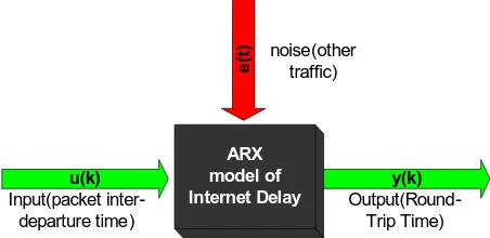
The end-to-end packet delay dynamics is modeled as a SISO (Single-Input-Single-Output) system. The input is the inter-departure times between packets leaving the source, and the output is an end-to-end packet delay measured at the destination. We use the Auto-Regressive eXogenous (ARX) model and determine its coefficients using system identification approach (Figure 5).
Since the ARX is a linear time-invariant model, it cannot rigorously capture the non-linearity of the packet delay dynamics. Nevertheless, the ARX model is applied in many control engineering problems, because non-lin- earity around a stable operating point can be well ap- proximated by a linear system.
e(
t)
ARX model of Internet Delay
u(k) y(k)
Output(Round-Trip Time) Input(packet
inter-departure time)
noise(other traffic)
[image:7.595.58.287.455.687.2] [image:7.595.309.535.598.708.2]The input of this system is the inter-departure times between packets leaving the source, and the output is an end-to-end packet delay measured at the destination. Ef- fects of other traffic and communication link such as the packets coming from other hosts are also modeled as noise in the ARX model. Due to the non stationary char- acteristics of the aggregated network traffic [27], in order to reduce non-stationarity of noise, instead of end-to-end packet delay itself, we use the end-to-end packet delay variation. The input to the ARX model is the inter-de- parture time (u[k]). In unilateral teleoperation applica-
tions, this is constant and determined by the control fre- quency. Therefore, given a constant input, the predicted output (end-to-end packet delay) would also become constant after the transient period. Therefore, the dy- namic model may appear to be unrelated for teleopera- tion applications, but in bilateral teleoperation, which is the main focus of our modeling applications, the model can be used.
However even in a unilateral teleoperation we can use random inter-departure times in order to address the de- lay effects on system dynamics. As the input to the sys- tem, we use a packet inter-departure time from the source,
i.e., the interval between two consecutive packet trans-
missions from the source. Use of the packet inter-depar- ture time is straightforward since, as suggested by the queuing theory, it directly affects the end-to-end packet delay. On the contrary, as the output from the system, we use an end-to-end packet delay variation measured by the destination, i.e., the difference in two consecutive end-
to-end packet delays.
Our approach of a black-box modeling using the ARX model is distinctive from other black-box approaches for modeling network traffic using the AR (Auto-Regressive) model or the ARMA (Auto-Regressive Moving Average) model [15,19,20,27].
3.3. Black-Box Modeling Using ARX Model
Here we have modeled the internet dynamics based on its delay dynamics as a single-input-single-output (SISO) system and the end-to-end packet delay dynamics are used to describe the dynamics of this SISO system. We use the ARX model and determine its coefficients using system identification techniques [23]. The ARX model has the input whereas either the AR model or the ARMA model does not have any input. In other words, only the ARX model provides us with how the past input data affects the future output data.
Nevertheless, the ARX model is a linear time-invariant model, therefore it cannot significantly capture non- linearity of the packet delay dynamics. However, the non-linear dynamical systems operating around a stable point can be well approximated by a linear system [21],
and the ARX model can be applied effectively to this system and to similar various control engineering prob- lems. Figure 5 illustrates the fundamental concept of using the ARX model for modeling the packet delay dy- namics.
The input to the ARX model is a packet inter-depar- ture time from the source, and the output from the ARX model is an end-to-end packet delay variation measured by the destination. Effects of other traffic (i.e., packets
coming from other hosts) are modeled as the noise. To determine the coefficients of the ARX model, a few sets of input and output data are collected from simulation using NS2 [22] and our own measurements.
u k as input and y
By considering k as output
data at slot k, the ARX model for this system can be
written as:
1 1 1 1 1 2 1 a a b b d n n n nA q y k B q u k n e k
A q a q a q
B q b b q b q
(1)
where e k
1 q
is un-measurable disturbance (i.e., noise),
and 1
1
q u k u k
is the delay operator;
i.e.,
n
n
. The numbers a and nb are the orders of respective polynomials. The number d is the number of delays from the input to the output. For brevity, we use as:
n n na, ,b d
(2)
u k and y
In this paper, k
a b
correspond to the
k-th packet inter-departure time and the k-th end-to-end
packet delay variation. All coefficients of the polynomi- als, n and n, are parameters of the ARX model, and are to be determined from the input and the output data using system identification.
The system identification problem for the ARX model is formulated as a minimization problem, where the cost function is given by a loss function [23]. Only the outline are shown in this paper, and interested readers are re- ferred to [23] for more detail. Let be a vector of all
coefficients and
k nab n
T 1, , na, , ,1 nb
a a b b
be a vector of all past out- puts and inputs, respectively. Then:
1 , , ,
1 , , a
d d b
k y k y k n
u k n u k n n
Using (1), the output from the ARX model y kˆ
is:
ˆ T
y k k (3)
The loss function , N
VN Z is defined as the sum of all squared prediction errors for the N input and output
2 ˆ y k 1 1 , N N N k V ZN y k
N
(4)
where Z is the past input and output data defined as:
1 , 1 , ,N
,
Z u y
ˆ
u N y N (5)
The solution N that minimizes the above loss func- tion is easily obtained by the least square method:
1ˆ T N k k k k
1 1 N Nk y k
(6)
The simulation model consists of 10 source-destina- tion pairs and a single bottleneck link. The exponential distribution is used as justified in [23]. The average transmission rate of UDP packets is set to 203 Kbit/s. Other simulation parameters are: the packet size is fixed at 2000 bytes, the bottleneck link bandwidth is 1.3 Mbit/s, the propagation delay of the bottleneck link is 1.8 ms, and propagation delays of access links range from 0.5 to 2 ms. We consider two cases: 1) each host sends only UDP packets and 2) each host sends both UDP and TCP packets.
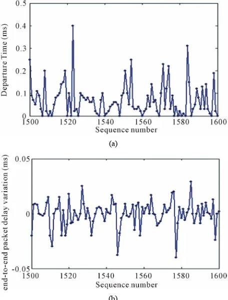
Figures 6 and 7 show the inter-departure time u k
and the end-to-end packet delay variation y k for the
UDP and the UDP + TCP cases, respectively. The end-
(a)
(b)
Figure 6. (a) The Packet inter-departure time and (b) end-to-end packet delay variation
(a)
(b)
Figure 7. (a) Packet inter-departure time and (b) end- to-end packet delay variation
u k
y k
in UDP + TCP case.
y
to-end packet delay variation k is measured, and the model output
u k
y k in UDP case.
y k is the simulated output from the ARX model:
T
y k k
where,
1 , , ,
1 , ,
a
d d b
k y k y k n
u k n u k n n
However, choosing different values for elements can effectively change the result of modeling, but the ARX model can correctly model the end-to-end packet delay dynamics if is chosen appropriately.
We choose 20, 20,1 for the UDP and UDP + TCP cases to minimize the AIC (Akaike’s Information Theoretic Criterion) [23-25]. The AIC is defined as:
2
AIC Log 1 , N
N
n
V Z
N
(7)
a b
n n n
where n is the number of unknown parameters, i.e.,
[image:9.595.59.287.399.698.2]end packet delay dynamics is modeled by the ARX model.
Of all data collected in previous section, we use the input and output data of 100 packets (1500 ≤ k < 1600)
for coefficients determination and model validation. As an example, when
6,6,1
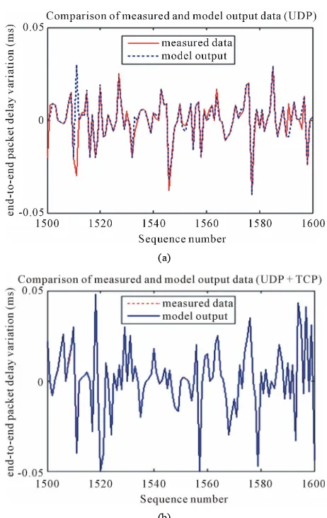
, coefficients of the ARX model and their standard deviations are shown in Table 3(a) (the UDP case) and 3(b) (the UDP + TCP case). Figures 8 and 9 compare the measurements and the model output for 20, 20,1
in the UDP case, and in the UDP + TCP case, respectively. It is evident that in both cases, the model output y kˆ
and the measure-ment y k
slightly differ. This is because the measuredend-to-end packet delay variation is disturbed by other unknown traffic not included in the model output y kˆ
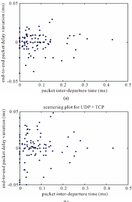
.To observe the correlation between u k
and y k
5
a a6
, scatter plots for the input and the output data of 1,000 packets are shown in Figures 10(a) and (b) for the UDP case and the UDP + TCP case, respectively. We note a weak negative correlation between the inter-departure time and the end-to-end packet delay variation. In spite of such a weak correlation, the ARX model can accu- rately capture the end-to-end packet delay dynamics. We have also have used this model to develop and verify teleoperation systems under various Internet delays. The experimental results confirm the accuracy and usefulness of our theoretical derivations [28,29].
4. Nonlinear Adaptive Control
[image:10.595.307.538.79.445.2]The important point in the remote operation system is the
Table 3. Coefficients and std. deviations of the ARX model for UDP case (a) and UDP + TCP (b).
(a)
1
a a2 a3 a4
Coefficient 0.261 0.248 0.282 0.136 0.053 0.231
Std. Dev. 0.112 0.115 0.114 0.111 0.108 0.013
1
b b2 b3 b4 b5 b6
Coefficient 0.004 0.021 0.282 0.0007 0.011 0.019
Std. Dev. 0.016 0.015 0.016 0.016 0.015 0.013
(b)
1
a a2 a3 a4 a5 a6
Coefficient 0.107 0.129 0.018 0.052 0.029 0.11
Std. Dev. 0.105 0.106 0.108 0.107 0.107 0.103
1
b b2 b3 b4 b5 b6
Coefficient 0.008 0.026 0.007 0.012 0.028 0.03
Std. Dev. 0.027 0.025 0.026 0.025 0.024 0.02
(a)
[image:10.595.58.286.495.735.2](b)
Figure 8. The comparison of measured end-to-end delay variation data y k and model output data y k for (a)
ˆ
UDP case, and (b) UDP + TCP case.existing of time delay with the path. Because in the internet the delay for send is different with receive one, so in systems of bi lateral in internet, there will be two variables T2(t) and T1(t). Such delay in system makes the
control difficult and decreases the workability. In order to decrease the effects of delay, the mentioned time in the remote operation, there have been done some works. In 1957 Mr. Smith presented a new approach called smith’s approach [14] for the above problem. In 1989, Anderson and song presented the distribution and passivity theory. In 1977, Jacouz and Niemeyer [6] used the wave variable approach in sending remote signals and they used passiv- ity theory for stability of the systems. In 1999, Park and Chow [23] used the sliding mode for designing the con- trols in the remote operation systems. Finally, in 2000, Elhaj et al. [23] proposed an “event oriented approach”
for the remote operation systems.
(a)
[image:11.595.58.289.83.458.2](b)
Figure 9. The error between measured end-to-end delay data y k
and model output y k for (a) UDP + TCP, ˆ
and (b) UDP case.remote slave manipulator (slave site). The human opera- tor controls the local master manipulator to drive the slave in order to perform a given task remotely (Figure 11).
The system must be completely “transparent” so that the human operator could feel as if he/she is able to di- rectly manipulate the remote environment. Instead of perfect force tracking, the overall teleoperation system should behave as a free-floating mass plus linear damper specified by the control and scaling parameters. Hung, Marikiyo and Tuan in [17] used the concept of a virtual manipulator to design a nonlinear control scheme that guarantees the asymptotic motion (velocity/position) tracking and has a reasonable force tracking performance even in when the acceleration, the values of dynamic parameters of manipulators as well as the models for human operator and the environment are not available. In the absence of friction and other disturbances, dynamic
(a)
[image:11.595.309.537.84.431.2](b)
Figure 10. scatter plots for input and output data in (a) UDP case, and (b) UDP + TCP case.
MASTER + SLAVE
Virtual master manipulato
r m m,X
X Xs,.Xs
man
F Fext
as F am
F
d F
Figure 11. Block diagram of the adaptive control system.
models of the master and the slave manipulators are:
e
,
,
am mam xm m m xm m m m xm m
as xt xs s s xs s s s xs s
F F M q X C q q X g q
F F M q X C q q X g q
(8) If the followings are achieved
,m s as ext
X t X t F F (9)
[image:11.595.311.536.476.593.2]d d p d
5.2. Passivity
interface. This requires knowledge of the manipulator acceleration, which in practice, is difficult to obtain. Moreover, there is a trade-off between motion tracking performance, force tracking performance, and system stability for a master-slave teleoperation system. In order to improve the performance, we increase the degree of freedom of the control system by utilizing a “virtual master manipulator”. This manipulator is described by the following dynamic model
d d d
F MM X K X K X
T T
m U Ut tV Vt t
[image:12.595.337.538.182.269.2](10)
Figure 8 shows the block diagram of the overall teleop- eration system using the virtual master manipulator.
5. Wave Variables
5.1. Definition of Wave Variables
The wave variables concept was proposed originally in [7,8] by Anderson and Spong, for teleoperators with communications delays. The concept of wave variables is based on a more general framework of passivity and was motivated by the case of scattered operators. For ease of reference, we repeat the basic mathematical formulations for the wave variables method using power flow as:
PX F (11)
in which the F and X denote force and velocity respect-
tively and U and V are incidental and reflected wave
variables in Figures 12 and 13. U and V can be calcu-
lated from power parameters (F and X) as:
, bX F U 2 2 bX F V b b
(12)
in which the parameter b is a positive constant depends
only on network and communication link characteristics. For a bilateral teleoperation of forced reflected sys- tems, the transmission process can be defined as:
,
s m
m s
U t T
V t T
0 E
U tV t (13)
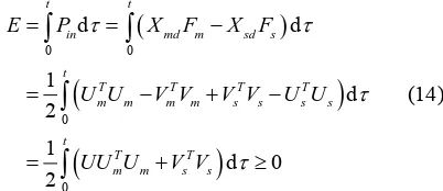
Transforming the power parameters into wave variables will affects on the system passivity. Using transmission process formula (13) in power flow relation (11) and with assuming the initial energy state 0 , the overall energy of communication link during signal transmission between master-slave will be calculated as:
where T is a constant time delay, and the m and s also
represents respectively the master and slave side of the waves. Here however the system is stable for any time delay (T), but the system performance decreases signifi-
cantly proportional to the time-delay in communication link.
0 0 0 0 d d 1 d 21 d 0
2
t t
in md m sd s
t
T T T T
m m m m s s s s
t
T T
m m s s
E P X F X F
U U V V V V U U
UU U V V
(14)where, Xmd and Xsd are the desired velocities of the mas- ter and the slave, respectively. The system is passive in- dependent of the delay T. This means the applied trans-
formation makes the wave variables robust against time-delay (constant delays). However this is gained at the cost of significant performance degradation for long delays. Using an observer or predictor in communication link may improve the efficiency at variable and long time-delays [12].
6. Smith Predictor
6.1. Structure of Smith Predictor
A very effective time delay compensation method is to use the Smith Predictor [13-15] as shown in Figure 14,
in which C s
P s
ˆP s
is the controller, is the plant that includes communication delay, is the plant model, and P sˆ
is the plant model without the time delay.Since the control signal is delayed, the same delay is ac-
+ m F s F + Delay Delay b 2b
2b s Fs
b 2 U b F U b 2 s s m X m U Us
m V Vs
s
[image:12.595.309.538.519.607.2]X
Figure 12. Transformation from power parameters to wave variables [5].
[image:12.595.111.484.650.721.2]
C(s) + P(s)
+ + (s) Pˆ (s) Pˆ_
e e
[image:13.595.309.537.80.360.2] r d y V u
Figure 14. Smith predictor block diagram.
counted for in the controller to coordinate the feedback with system dynamics. The Smith Predictor works poorly unless the delay is precisely known [16].
6.2. The Multivariable Smith Predictor
However the Smith Predictor is typically used for Single- Input-Single-Output (SISO) systems, here we have ex- tended the concept of smith predictor to be applied in a multivariable system. Considering P s
and P sˆ
12 22 e e e , e e T S T S s s
1ˆ
PC I PC
as transfer matrices:
11 21 11 12 21 22 11 12 21 22 ˆ T S Ts T SP s P
P s
P s P
P s P s
P s
P s P s
(15)
So the closed-loop system can be defined as follow:
cl
P s (16) This shows that similar to the SISO system, in multi- input-multi-output (MIMO) systems also the delay can be also removed from the control loop.
6.3. Wave-Based Prediction and Regulation
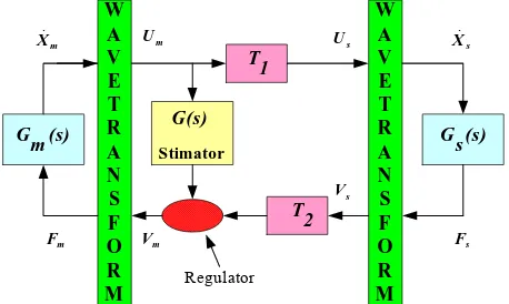
In order to overcome the limitations affected by using wave variables or smith predictor and to use their advan- tages at the same time, Munir [12] proposed a system includes the combination of smith predictor and wave- variables (we call it wave-predictor). Two different im- plementation schemes of this wave prediction technique are depicted in Figures 15(a) and (b). To preserve the properties of the stability and tracking, we have added additional features to the communication channel as shown in Figure 16.
7. The Wave-Variable Based Multi-Model
Adaptive Control System (MMACS)
Switching control systems are mainly proper to describe the abrupt and significant changes of dynamic systems. These variations may be due to the failure of the compo- nent, disturbances, change in subsystem interconnections,
(a)
(b)
Figure 15. Prediction inside the wave domain (a) and an alternative implementation (b).
m
F Fs
m
X Um Us
[image:13.595.59.285.83.191.2]m V s V s X W A V E T R A N S F O R M (s) m G 1 W A V E T R A N S F O R M T 2 T G(s) (s) s G Stimator Regulator
Figure 16. Block diagram of the wave-based communication system with prediction and regulation.
environment changes and repairs [18-21]. When a single identification model is used, it will have to adapt itself to the operating condition before appropriate controls can be taken. If the environment changes suddenly, the original model (and hence the controller) is no longer valid.
If the adaptation is slow, it may result in a large tran- sient error. However, if different models are available for different operating conditions, then suitable controllers corresponding to each condition can be devised in ad- vance.
[image:13.595.309.538.403.540.2]
1 Controller 2 Controller N Controller
1 Model 2 Model
N Model
1
u 2 u
N
u
y
1
~
y
2
~y
N
y
~
1 e
2
e
N
e
(a)
[image:14.595.126.470.81.458.2](b)
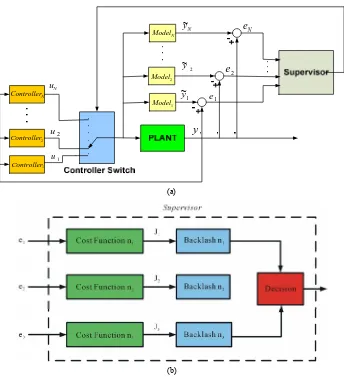
Figure 17. Multi-model adaptive control system and the supervisor operation.
instant, and activates the corresponding controller. This structure is based on N models which have been devel- oped at various points across the operating range of the process.
A controller is designed for each model, using the Dio- phantine pole-placement algorithm. A supervisor as shown in Figure 17(b) compares the output errors for each one of the N models. A discrete equivalent of the performance index is given in (17), for the th model:
i
e2
M exp
e2
i i
1
i i
j
J k k
j kj
(17)
Expansion of this controller for the master-slave teleoperation was proposed in [22], where the best model for the current operating condition is identified and the corresponding controller either in the master or in the slave is activated. The block diagram of this proposed control system is shown in Figure 18. Here we have used the ARX model for the communication delay, and ob- tained its parameters using a system identification ap- proach; and studied its performance under abrupt
changes in the time delay using simulation and analysis. The stability of the proposed MMAC system [30] will preserved by: limJ ki
0. In a Linear Time Invariant(LTI) Multi-Model Adaptive Control (MMAC) system, the end result is a conventional adaptive model, i.e. there
exists a time t1 then after tt1 we have J ti
and the switching stops. Hence, for a LTI MMAC, the closed loop system is BIBO stable [31].
This technique has been applied to control a simple teleoperation system and its behaviour for a constant delay and also a time-varying delay on the communica- tion link between the plant and the controller has been studied.
Figure 19(a) shows the system output using ordinary wave prediction method. In the output of our proposed method (Figure 19(b)) we note that the proposed control system is more robust with minim overshoot.
Figures 19(c) and 20 show the step responses for ordi- nary and proposed control methods, when time delay changed abruptly from 700 msec to 2100 msec at t = 50.
Figure 18. Proposed multi-model adaptive control system block diagram for teleoperation via the internet.
(a) (b)
(c)
Figure 19. The step response of the system while using traditional wave-variable prediction technique (a), using proposed MMACS technique (b), and comparing the traking response of these two techniques in abrupt time-delay variation (c).
has a satisfactory response with small fluctuations. Fig- ure 21(a) shows the tracking response without wave pre-
[image:15.595.60.538.315.661.2]the environment’s parameters.
In order to examine the tracking efficiency of the pro- posed control, the system tracking response without wave pr
oper platform in this paper. ediction, with wave prediction and also with proposed control system in constant time delay (2 sec) are depicted in Figures 22(a)-(c). Here we have also examined dif- ferent configuration of wave variable block combined with the MMAC system. Two different structures are implemented as depicted in Figures 23(a) and (b). Simu- lation results of the control signals using wave variables and estimator in constant and also in variable (1 ± 0.02 sec) delays are shown in Figures 24 and 25 for these configurations. Comparing these plots show that the se- cond configuration (placing MMAC between master and slave) introduces a more efficient characteristics.
8. Conclusion and Future Works
The dynamics of internet as a possible pr for real-time teleoperation were addressed
[image:16.595.62.539.342.707.2]The internet delay dynamics were introduced as a main
Figure 20. comparision of the traking response of the pro- posed technique with the ordinary wave-based prediction technique in abrupt time-delay variation (at t = 200 s) shows the robustness and efficiency of the proposed method.
(b) (a)
(c)
wave prediction (a) and the system output tracking response with l system (c) in variable time delay (1 ± 0.02 sec).
Figure 21. System tracking response without wave predict-
(a) (b)
(c)
Figure 22. (a) System tracking response without wave predictio ) system output tracking response with wave prediction and (c) the system tracking response with proposed control syste constant time delay (2 sec).
n (b m in
[image:17.595.60.541.83.505.2](a)
[image:17.595.108.489.548.717.2][image:18.595.60.539.84.286.2]
(a) (b)
Figure 24. Simulation of the control signals using wave va s and estimator (Figure 20(a)) in constant delay (a) and in variable (1 ± 0.02 sec) delay (b).
riable
(a)
Figure 25. Position tracking in proposed augmented structu gure 20(b)) in constant delay (a) and in variable (1 ± 0.02 sec delay (b).
ased teleoperation. Characteristics of the internet delay
with these time delay variation. We note that the pro-
response with small fluctuations. The results indicate the (b)
re (Fi )
QoS parameter to define the constraints for internet- posed multi-model control strategy has a satisfactory b
dynamics were extracted using delay measurement in several real internet nodes. Using measurement results a block-box model for internet delay dynamics were in- troduced and applied for modelling internet dynamics in web-based teleoperation system. We showed a regular cyclic behaviour in despite of the irregular and chaotic nature of the internet time-delay dynamics, and also abrupt and significant changes in delay dynamics. In or- der to overcome the limitation of the previously proposed works to deal and describe this abrupt variation, we de- veloped a new adaptive control system which fully adapt
usefulness of our proposed approach particularly for abrupt variations of the environment’s parameters. This structure can also be combined with the wave variable method, the Smith predictor method, and a combination of the two in linear and/or nonlinear controllers, time- based and/or non-time based controllers and other suit- able types of controllers, so that the most fitting control- ler can be utilized depending on the circumstances.
9. Acknowledgements
[image:18.595.60.537.327.527.2]Prof. M. Sawan, Prof. A. R. Sharafat and Prof. H. R. Mo- meni.
REFERENCES
evice for Micro-Manipulation,” International Journal of Robotics and Automation, Vol. 26, No. 3, 2011, pp.
247-254. doi:10.2316
[1] K. Houston, A. Sieber, C. Eder, O. Vittorio, A. Menciassi and P. Dario, “A Teleoperation System with Novel Haptic D
/Journal.206.2011.3.206-3224
[2] H.-J. Liu and K.-Y. Young, “Applying W ave-Variable-Based Sliding Mode Impedance Control for Robot Tele- operation,” International Journal of Robotics and Auto- mation, V. 26, No. 3, 2011, pp. 296-304.
doi:10.2316/Journal.206.2011.3.206-3440
[3] K. Brady and T. J. Tarn, “Internet-Based Remote Teleop- eration,” Proceedings of IEEE International Conference of Robotics and Automation, Leuven, 16-20 May 1998,
pp. 65-70.
[4] T. J. Tarn and K. Brady, “A Framework for Time-Delayed Telerobotic Systems,” P
the Control of
roceedings o
ystem in Teleoperation,”
Robotics Research, Vol. 17, No. 4, 1998, pp f IFAC Robot Control, Nantes, 3-5 September 1997, pp.
599-604.
[5] N. Hung, T. Marikiyo and H. Tuan, “Nonlinear Adaptive Control of Master-Slave S
trol Engineering Practice, Vol. 11, 2003, pp. 1-10.
[6] R. Oboe and P. Fiorini, “A Design and Control Environ- ment for Internet Based Telerobotics,” International
Journal of .
433-499. doi:10.1177/027836499801700408
[7] G. Niemeyer and J. E. Slotine, “Using Wave Variables for System Analysis and Robot Control,” Proceedings o
sactions on f IEEE International Conference of Robotics and Automa- tion, Albuquerque, 20-25 April 1997, pp. 1619-1625. [8] R. J. Anderson and M. W. Spong, “Bilateral Control of
Teleoperators with Time Delay,” IEEE Tran Automatic Control, Vol. 34, 1989, pp. 494-501. doi:10.1109/9.24201
[9] R. J. Anderson, “SMART Class Notes,” Intelligent Sys-tems & Robotics Center, Sandia National Laboratories
ol, Vol .
ence of Robotics and Automation,
Leu-me-Varying Communication
De-ased Teleoperation
on Systems Design Using Augmented Wave-Vari-
, No. 6, 1980, pp. 937-949.
,
. Livermore, 1994.
[10] G. Niemeyer and J. E. Slotine, “Stable Adaptive Teleop-eration,” IEEE Transactions on Automatic Contr
36, 1991, pp. 152-162
[11] G. Niemeyer and J. E. Slotine, “Toward Force-Reflecting Teleoperation over the Internet,” Proceedings of IEEE In- ternational Confer
ven, 16-20 May 1998, pp. 1909-1915.
[12] Y. Yokokohji, T. Imaida and T. Yoshikawa, “Bilateral Teleoperation under Ti
lay,” Proceedings of IEEE/RSJ International Conference of Intelligent Robots and Systems, Vol. 3, 1999, pp. 1854-
1859.
[13] S. Munir and W. J. Book, “Internet-B
Using Wave Variables with Prediction,” IEEE/ASME Tran- sactions on Mechatronics, Vol. 7, No. 2, 2002, pp. 124- 133.
[14] S. Ganjefar, H. R. Momeni and F. Janabi-Sharifi, “Tele-
operati
ables and Smith Predicator Method for Reducing Time- Delay Effects,” Proceedings of International Symposium on Intelligent Control, Vancouver, 27-30 October 2002,
pp. 27-30.
[15] J. M. Smith, “Closer Control of Loops with Dead Time,”
Chemical Engineering Progress, Vol. 53, No. 5, 1957, pp.
217-219.
[16] Z. Palmor, “Stability Properties of Smith Dead-Time Compensator Controllers,” International Journal of Con- trol, Vol. 32
doi:10.1080/00207178008922900
[17] W. J. Book and M. Kontz, “Teleoperation of a Hydraulic Forklift from a Haptic Manipulator over the Internet,”
upervisory Con-tion and Closed-Loop
on Auto-
George W. Woodruff School of Mechanical Engineering, Georgia Institute of Technology, Atlanta, 2003.
[18] E. Mosca and T. Agnoloni, “Switching S trol Based on Controller Falsifica
Performance Inference,” Dipartimento di Sistemi Infor-matica, Universita di Firenze, Firenze, 2002.
[19] K. S. Narendra and J. Balakrishnan. “Adaptive Control Using Multiple Models,” IEEE Transactions
matic Control, Vol. 42, No. 2, 1997, pp. 171-187. doi:10.1109/9.554398
[20] K. S. Narendra, J. Balakrishnan and M. K. Ciliz, “Adap- tation and Learning Using Multiple Models, Switching, and Tuning,” IEEE Control Systems Magazine, Vol. 15,
No. 3, 1995, pp. 37-51. doi:10.1109/37.387616
[21] L. Chen and K. S. Narendra, “Nonlinear Adaptive Contro Using Neural Network
l s and Multiple Models,” Scientific
ration via
via Inter-
g System Identification,” Proceed-
rani, A. Ramazani and F. Monteiro,
“Teleopera-omeni and A. R. Sharafat, “A Novel
and A. R. Sharafat, “Model- ing Internet Delay Dynamics for Teleoperation,” Procee-
Systems Company Inc., Woburn, and Center for Systems Science, Yale University, New Haven, 2001.
[22] E. Kamrani, H. R. Momeni and A. R. Sharafat, “A Multi- Model Adaptive Control System for Teleope
Internet,” Proceedings of the IEEE International Confer- ence on Control Applications, Taipei, 2-4 September
2004, pp. 1336-1340.
[23] E. Kamrani, “Control of Teleoperation Systems
net: Robustness against Delay,” Master’s Thesis, Science in Electrical Engineering, Faculty of Engineering, Tehran, 2005.
[24] E. Kamrani and M. H. Mehraban, “Modeling Internet Delay Dynamics Usin
ings of the 2005 IEEE International Conference on Indus- trial Technology (ICIT2006), Mumbai, 15-17 December
2006, pp. 716-721. [25] E. Kam
tion via Internet with Time-Varying Delay,” Proceedings of the 13th IEEE International Conference on Electronics, Circuits and Systems (ICECS 2006), NICE, 10-13 De-
cember 2006, pp. 736-739. [26] E. Kamrani, H. R. M
Adaptive Control System for Stable Teleoperation via Internet,” Proceedings of 2005 IEEE Conference on Con- trol Applications, Toronto, 28-31 August 2005, pp. 1164- 1169.
dings of 2005 IEEE Conference on Control Applications
(CCA 2005), Toronto, 28-31 August 2005, pp. 1528-1533. doi:10.1109/CCA.2005.1507349
[28] H. R. Karampoorian and E. Kamrani, “Modeling Internet Delay Dynamics: Comparative Study,” Proceeding of the
orld Applied Sciences
ol. 34, No. 2,
p. 4010-4015. 4th IASTED Asian Conference on Communication Sys-
tems and Networks (AsiaCSN’07), Phuket, ACTA Press,
Anaheim, 2007, pp. 233-238.
[29] M. Ghanbari and E. Kamrani, “Optimal Control of Robot through Internet,” International W
[32]
Journal, Vol. 6, No. 5, 2009, pp. 702-710.
[30] X. Y. Gu and W. Wang, “On the Stability of a Self-Tun- ing Controller in the Presence of Bounded Disturbances,”
IEEE Transactions on Automatic Control, V
1989, pp. 211-214.
[31] G. C. Goodwin and K. S. Sin, “Adaptive Filtering: Pre-diction and Control,” Prentice Hall, Englewood Cliffs, 1984.
S. Hirche and M. Buss, “Packet Loss Effects in Passive Telepresence Systems,” Decision and Control, Vol. 4,