Abstract— This paper extends the sequential growing and pruning radial basis function (GAP-RBF) to cater for on-line identification of non-linear systems. Some desired modifications on the growing and pruning neurons criteria have been proposed for the original GAP-RBF to make it more suitable for on-line identification. The unscented kalman filter (UKF) has been proposed as a new learning algorithm for GAP-RBF neural network. Moreover, a variable forgetting factor strategy has been included in the UKF algorithm to keep the parameter estimation routine more active in time-varying dynamics. Simulation results show the superiority of the modified GAP-RBF (MGAP-RBF) neural network being learned with the UKF algorithm.
Index Terms— Adaptive on-line identification, GAP-RBF, MRAN, EKF, UKF.
I. INTRODUCTION
Many engineering applications need a suitable model structure, within which a good model is to be found, for a compact and accurate description of the dynamic behavior of the system under consideration. These models are used for simulations, predictions, analysis of the system’s behavior, design of model-based controllers, and so forth. Radial Basis Function (RBF) networks have been popularly used in many applications in recent times due to their ability to approximate complex nonlinear mappings directly from the input-output data with a simple topological structure and ease of implementation of dynamic and adaptive network architecture. In practical on-line applications, sequential learning algorithms are generally preferred over batch learning algorithms as they do not require retraining whenever a new data is received.
Manuscript received July 22, 2007.
M. R. Jafari is with the Automation and Instrumentation Department, Petroleum University of Technology, Tehran, Iran (e-mail: [email protected]).
T. Alizadeh is with the Automation and Instrumentation Department, Petroleum University of Technology, Tehran, Iran (e-mail: [email protected]).
M. Gholami is with the Automation and Instrumentation Department, Petroleum University of Technology, Tehran, Iran (e-mail: [email protected]).
A. Alizadeh is with Bonab Faculty of Engineering, University of Tabriz, Tabriz, Iran (e-mail: [email protected]).
K. Sahalshoor is with the Automation and Instrumentation Department, Petroleum University of Technology, Tehran, Iran (e-mail: [email protected]).
However, selection of a learning algorithm for an on-line application is critically dependent on its accuracy and speed. In recent years different methods like [1], [2] and [3] have been proposed in which sequential learning algorithms are used. A significant contribution to sequential learning was made by Platt [4] by proposing RAN in which hidden neurons were added sequentially based on the novelty of the new data. One important point to be noted in all of these sequential algorithms is that they do not link the required learning accuracy directly to the algorithm. Instead, they all have various thresholds which have to be selected using exhaustive trial and error studies. This issue of specifying the various thresholds based on the needed accuracy has been raised in MRAN for determining the inactive neurons, but the required learning accuracy was implemented in GAP-RBF [5] networks more clearly. The enhanced growing criterion proposed in the GAP-RBF algorithm will ensure that a neuron will not be added if it is insignificant to the overall performance of the network, even though it may make contribution to the single latest input data. GAP-RBF has much less computational complexity and requires less memory. Also GAP-RBF in comparison with RAN, RAN-EKF and MRAN has very few parameters for which one needs to select values for. The self-generating structure and low computational complexity of GAP-RBF make it one of the best candidates for on-line identification of complex systems with poor prior dynamic’s knowledge.
This paper focuses on the GAP-RBF and MRAN algorithms. The usual EKF learning algorithm has been upgraded to the UKF learning algorithm. An exponential forgetting factor strategy has been included in the UKF learning algorithm in order to enable it for tracking any possible time-varying dynamic changes. To make the neurons growing and pruning procedure more adapted to the on-line identification applications, the corresponding criteria have been modified. The rest of this paper is organized as follows. Section 2 describes GAP-RBF neural network briefly. Section 3 presents UKF learning algorithm. Section 4 describes the problems in the original GAP-RBF neural network and presents a modified GAP-RBF (MGAP-RBF) neural network. Section 5 presents performance comparison for the original GAP-RBF and its modified version on benchmark problems. Section 6 summarizes the resulting conclusions.
On-line Identification of Non-Linear Systems
Using an Adaptive RBF-Based Neural Network
II. GAP-RBFNEURAL NETWORK
GAP-RBF uses the Gaussian RBF network (GRBF) model. The network output vector f(xn), which approximates the
desired output vector yn, are described as follows:
∑
= = K k n k k n x x f 1 ) ( )( α φ (1) where
α
k is it’s connecting weight to the output neuron, and)
(
n kx
φ
denotes a response of the kth hidden unit to the inputs xn ;φ
k(
x
n)
is a Gaussian function given by:⎟ ⎟ ⎠ ⎞ ⎜ ⎜ ⎝ ⎛ − − = 2 2 exp ) ( k k n n k x x σ µ
φ (2)
where
µ
k andσ
k are the center and width of the Gaussian function respectively, and.
denotes the Euclidean norm.The sequential learning algorithm for GAP-RBF networks, defines a notion of significance for the hidden neurons, and a growing and pruning criterions for on-line adjusting of the network size.
A. GAP-RBF Learning Algorithm
During the sequential learning process, a series of training samples (
x
i,
y
(
x
i)
); (i = 1,2,...) are randomly drawn and presented one by one to the network. Each training sample would trigger the action of adding a new hidden neuron, pruning the nearest hidden neuron, or adjusting the parameters of the nearest hidden neuron, based on only the significance of the nearest hidden neuron to the training sample. This is in contrast with the MRAN learning algorithm in which all the neurons will be checked for adding, pruning and adjusting purposes. The significance of the kth hidden neuron k is defined as [5]:)
(
)
8
.
1
(
)
(
X
S
k
E
k l k sigα
σ
=
(3)Given the set of all hidden neurons in A, the center of the nearest hidden neuron is cr, the input is x and the nearest hidden
neurons are defined as:
⎭
⎬
⎫
−
=
−
∨
∈
⎩
⎨
⎧
=(
))
min
(
)
(
|
,...,1 K i
i r r
r
c
A
x
c
x
c
µ
(4)Like MRAN and EMRAN, the GAP-RBF network begins with no hidden neurons. As new observations are received during the training, some of them may initiate new hidden neurons according to the growing criterion. An enhanced growing criterion for new observation (xn,yn), to make the growing
process smooth is:
⎪
⎪
⎪
⎩
⎪
⎪
⎪
⎨
⎧
>
−
>
>
−
min min)
(
)
8
.
1
(
e
X
S
e
c
x
e
e
c
x
n l r n n n r nκ
ε
(5)If these conditions are satisfied, then a new K+1 neuron will be added and the parameters associated with the new hidden neuron are taken as follows:
⎪
⎩
⎪
⎨
⎧
−
=
=
=
+ + + r n K n K n Kc
x
x
c
e
κ
σ
α
1 1 1 (6)where en= yn - f(xn) and cr is the centre of the nearest hidden
neuron to xn. As the training carries on, some of the new
observations may trigger the learning algorithm to prune some hidden neurons.
The pruning criterion based on the new observation (xn ,yn) is:
min
)
(
)
8
.
1
(
)
(
e
X
S
k
E
k l ksig
=
<
α
σ
(7)where S(X) is the estimated size of the input range.
If the average contribution made by the kth neuron in the whole range X is less than the expected accuracy emin and the kth
neuron is insignificant; then the kth neuron can be removed. If no neuron adds or prunes, the nearest neuron will be adjusted with the EKF or UKF algorithm.
The complete description of the GAP-RBF learning algorithm [5] can be summarized as follows:
Given an approximation error emin, for each observation
(xn ,yn), where
l n
x
∈
ℜ
, do1. compute the overall network output
∑
=⎟⎟
⎠
⎞
⎜⎜
⎝
⎛
−
−
=
K k k n k k nx
x
f
1 2 21
exp
)
(
µ
σ
α
(8)where K is the number of hidden neurons.
2. calculate the parameters required in the growth criterion
)
(
)
1
0
(
},
,
max{
max minn n n n n
x
f
y
e
=
−
<
<
=
ε
γ
ε
γ
ε
(9)apply the criterion for adding neurons
If
e
n>
e
min andx
n−
µ
nr>
ε
n andmin
)
(
/
)
8
.
1
(
x
e
nS
X
e
l nr
n
−
µ
>
κ
allocate a new hidden neuron K + 1 with
adjust the network parameters
α
nr,
µ
nr,
σ
nr for the nearest neuron only, using the EKF algorithm.Check the criterion for pruning the hidden neuron: If
(
1
.
8
)
nr/
S
(
X
)
e
minl
nr
α
<
σ
, remove the nearest (nrth)hidden neuron and do the necessary changes in the EKF algorithm.
III. UNSCENTED KALMAN FILTER (UKF)
The inherent flaws of the EKF are due to its linearization approach for calculating the mean and covariance of random variables which undergoes a non-linear transformation. As shown in [2], [6] and [7], the UKF addresses these flaws by utilizing a deterministic “sampling” approach to calculate mean and covariance terms. This approach results in approximations that are accurate to the third order (Taylor series expansion) for Gaussian inputs for all nonlinearities.
For non-Gaussian inputs, approximations are accurate to at least the second-order [2]. Whereas, the linearization approach of the EKF results only in first order accuracy.
Consider the non-linear system, described by (11). The UKF algorithm can be derived by the following steps:
k k k k k k k k
v
x
h
y
w
u
x
f
x
+
=
+
=
+)
(
)
,
(
1 (11) 1. Initialize with:]
)
ˆ
)(
ˆ
[(
]
[
ˆ
0 0 0 0 0 0 0 Tx
x
x
x
P
x
x
−
−
Ε
=
Ε
=
(12) fork
∈
{
1
,...,
∞
}
, (E[.] denote the expected value). 2. Calculate the sigma points:⎥
⎥
⎦
⎤
⎢
⎢
⎣
⎡
−
+
=
− − − − −−1
ˆ
k 1ˆ
k 1 k 1ˆ
k 1 k 1k
x
x
γ
P
x
γ
P
χ
(13)3. Time update:
[
1 1]
* 1
|k−
=
k−,
k−k
F
χ
u
χ
(14)∑
= −
−
=
Li k k i m i k
W
x
2 0 * 1 | , ) (ˆ
χ
(15)[
] [
]
∑
= − − − −−
=
L−
−
+
i w T k k k i k k k i c i
k
W
x
x
R
P
2 0 * 1 | , * 1 | , )(
χ
ˆ
χ
ˆ
(16) where w
R
is process noise covariance, and⎥
⎥
⎦
⎤
⎢
⎢
⎣
⎡
−
+
=
− − − − −− k k k k k
k
k
x
x
γ
P
x
γ
P
χ
| 1ˆ
ˆ
ˆ
(17)]
[
| 1 1| −
=
−Υ
kkh
χ
kk (18)∑
= −
−
=
LΥ
i k k i m i k
W
y
2 0 1 | , ) (ˆ
(19) 4. Measurements update equations:[
] [
]
v L i T k k k i k k k i c i yy
W
y
y
R
P
k
k
=
∑
Υ
−
Υ
−
+
= − − − − 2 0 1 | , 1 | , )
(
ˆ
ˆ
(20) where v
R
is process noise covariance, and⎥
⎥
⎦
⎤
⎢
⎢
⎣
⎡
−
+
=
− − − − −− k k k k k
k
k
x
x
γ
P
x
γ
P
χ
| 1ˆ
ˆ
ˆ
(21)[
] [
]
∑
= − − −−
−
Υ
−
=
L i T k k k i k k k i c i yx
W
x
y
P
k k 2 0 1 | , 1 | , )(
ˆ
ˆ
χ
(22)1
−
=
Κ
kP
xkykP
ykyk (23))
ˆ
(
ˆ
ˆ
=
−+
Κ
−
−k k k k
k
x
y
y
x
(24)T k y y k k
k
P
P
k kP
=
−−
Κ
Κ
(25)IV. THE MODIFIED GAP-RBFNEURAL NETWORK AND THE
MODIFIED UKFLEARNING ALGORITHM
The proposed modifications can be described in two sections. First, changes in the GAP-RBF algorithm and second on the UKF learning method.
A. The Modified GAP-RBF Neural Network
In order to have smoothly output response and avoid oscillation, the mechanism of adding and pruning should be allowed to change smoothly. The rate of adding or pruning of neurons can be controlled with threshold values of en and
ε
n. Selection of these values depends on the complexity of the system, input data for identification and the required accuracy for the model. But the most important and effective factor is the persistent exciting (PE) of the input data. If the input data have enough degree of PE, smooth and accurate output can be obtained with suitable adjusting of the threshold values, but if the inputs do not be PE, which may happen for instance in the case of closed-loop identification, then the threshold values can not help and hence modification on adding and pruning rules will be necessary.In on-line identification, it should be better to change the adding strategy in such a way that, the rate of adding neurons increased in the beginning of the identification process, and as the identification process continues on, the rate of adding neurons decreased. In the original algorithm [5], and its applications [1], [5] and [8], neurons are added hardly in the start of the modeling process. This causes large errors in the start of the algorithm and hence the learning EKF or UKF techniques can not estimate the relevant parameters. As the rate of neuron creation can be controlled with
ε
n, an exponential function is proposed to be used in order to increaseε
n as follows:)
1
)(
(
/ min maxmin
ε
ε
τε
ε
n ne
−−
−
+
=
(26)Another problem is due to oscillation in the number of created neurons that can cause big errors in the identification results. This oscillation will be occurred in on-line identification, when the numbers of neurons that are created are small and the inputs data have small degree of PE, too. The effects of mentioned problem can be reduced with changing the pruning criteria by adding a new pruning factor (
β
) as follows:min
)
(
/
)
8
.
1
(
σ
nr lα
nrS
X
<
β
e
(27) where0
<
β
≤
1
.B. The Modified UKF Algorithm
In on-line identification, learning algorithms should be fast. However, to accomplish this objective, the initial value of the covariance matrix can not be set at large value because this option will produce large error and hence the neural network output will oscillate and consequently can not be converged when other samples are received. Besides small initial value of the covariance matrix has another bad effect. This slows down the identification process, which is not acceptable in the on-line applications. In order to be able to track any dynamic changes efficiently, learning algorithms should be fast enough to be converged in a few number of iterations. A factor, called as
η
, is proposed to be used in the UKF algorithm which acts as the forgetting factor concept in the usual recursive least squares (RLS) algorithm.When the GAP-RBF toggles to adjust the parameters,
η
is reset to the initial value, and then it changes exponentially in such a way that the final value is reached in a few number of iterations. As a consequence, the modified equation is as follows:k T k y y k k
k
P
P
k kP
=
(
−−
Κ
Κ
)
/
η
(28) where)
1
)(
1
(
/1
1
η
δη
η
tk k
k
e
− −
−
+
−
−
=
,0
<
η
k≤
1
(29)where t is the time duration that is spent during which the GAP-RBF toggles to the UKF learning algorithm. t is then reset to zero when the GAP-RBF algorithm is exited from the UKF.
δ
is the parameter that controls the rate of changing inη
.V. SIMULATION RESULTS
In this section, the identification capabilities of the modified GAP-RBF neural network with the modified UKF learning algorithm are tested on a benchmark problem. The resulting performances are compared with the original GAP-RBF neural network being estimated with both the EKF and UKF learning algorithms.
A. Nonisothermal Continues Stirred Tank Reactor (nonisothermal CSTR)
The process is a nonisothermal CSTR with an irreversible
reaction (A
→
B) which consists of two nonlinear ordinary differential equations, given by [9]:),
(
)
exp(
)
(
0t
RT
E
C
k
C
C
V
q
dt
dC
c A
A Af
A
=
−
−
−
φ
(30)
)
(
)
(
exp
1
)
(
)
exp(
)
(
)
(
0T
T
t
C
q
hA
q
V
C
C
t
RT
E
C
C
k
H
T
T
V
q
dt
dT
cf h
pc c c
p pc c
c p
A f
−
×
⎥
⎥
⎦
⎤
⎢
⎢
⎣
⎡
⎟
⎟
⎠
⎞
⎜
⎜
⎝
⎛
−
−
+
−
∆
−
+
−
=
φ
ρ
ρ
ρ
φ
ρ
(31)
where
)
(
t
h
φ
fouling coefficient)
(
t
c
φ
deactivation coefficientA
C
effluent concentration, ( the controlled variable) cq
coolant flow rate, (the manipulated variable) q feed flow rate, disturbanceAf C
feed concentration f
T
feed temperature cfT
coolant inlet temperatureThe remaining model parameters together with the operating conditions are presented in Table 1.
This CSTR has a time-varying characteristic given by: A
h h
d
t
h
t
h
h
=
φ
(
)
×
=
(
1
−
α
)
whereα
h=
0
.
01
is fouling constant.The free parameters have been fixed in all the experiments as follows in order to be able to compare and analyze the experiments results at the same conditions:
=
max
ε
0.1,ε
min=
0.01,κ
=
0.85,γ
=
0.995 and emin=0.001.In order to make the picture of the performed simulation experiments more real, two distinct white noises with variance of 0.01 have been added to the original dynamics in (30) and (31) to simulate as the process noises. Since the effluent concentration (CA) has been assumed as the process output, a white noise with variance of 0.01 has also been added to it as the measurement noise.
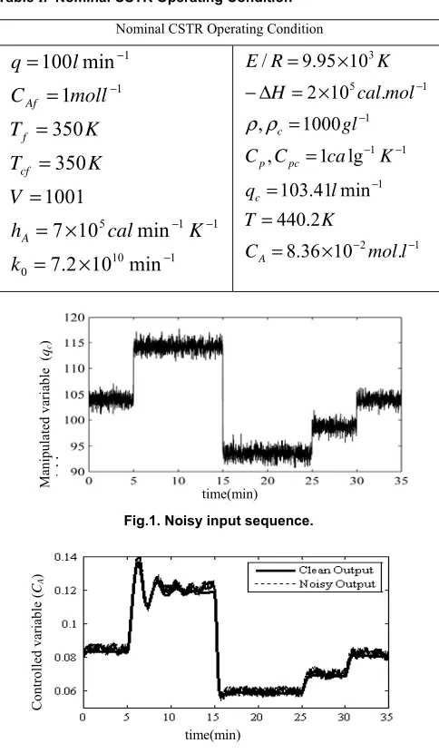
Table І. Nominal CSTR Operating Condition
Nominal CSTR Operating Condition
1 10 0
1 1 5
1 1
min
10
2
.
7
min
10
7
1001
350
350
1
min
100
− − − −
−
×
=
×
=
=
=
=
=
=
k
K
cal
h
V
K
T
K
T
moll
C
l
q
A cf f Af
1 2
1 1 1 1
1 5
3
. 10 36 . 8
2 . 440
min 41 . 103
lg 1 ,
1000 ,
. 10 2
10 95 . 9 /
− −
− − − −
−
× = =
= = =
× = ∆ −
× =
l mol C
K T
l q
K ca C C
gl mol cal H
K R
E
A c
pc p
c
ρ
ρ
Fig.1. Noisy input sequence.
Fig. 2. Real (noisy) and clean CSTR output
[image:5.595.315.515.85.691.2]The obtained process output response has been illustrated in Fig.2 together with a non-real noise-free process output response for the demonstration purposes.
The complete identification results for different performed experiments with GAP-RBF and MGAP-RBF algorithms have been shown in Fig. 3. In Fig. 3 (a-c) vertical axis is output concentration (CA) and in Fig. 3 (d-f) the vertical axis is the
number of created neurons.
(a)
(b)
(c)
(d)
(e)
(f)
Fig. 3. Approximated network output and neuron updating progress. (a)-(c) GAP-EKF, GAP-UKF, MGAP-UKF output networks respectively. (d)-(f) neuron updating progress of mentioned networks.
Ma
nipulate
d v
aria
ble (
qc
)
ariab
le
time(min)
time(min)
C
ontrolled var
iable (
CA
)
time(min)
Output (
CA
)
Output (
CA
)
time(min)
O
utput
(
C
)
time(min)
N
um
be
r of
N
eurons
time(min)
N
um
be
r of
N
eurons
time(min)
time(min)
Nu
m
ber o
f
N
[image:5.595.47.289.91.506.2] [image:5.595.63.257.624.746.2]The results demonstrate the superiority of the proposed MGAP-RBF-UKF algorithm with respect to other algorithms in terms of the following two main objectives:
1. Network model accuracy in terms of Integral of Squared Error (ISE) measure.
2. Network model structure simplicity or compactness of number of neurons.
Table ІІ. Performance Comparison of Different Neural Networks
Type of NN ISE
GAP-EKF 0.2057
GAP-UKF 0.1646
MGAP-UKF 0.0276
VI. CONCLUSIONS
Two different types of adaptive neural networks, i.e. GAP-RBF with EKF and UKF learning algorithms and MGAP-RBF have been utilized for on-line identification of non-linear systems. In this paper, this original network structure has been modified in order to enable their applications for on-line identification purposes. The basic contributions can be summarized as follows:
• Modification in neuron creation criterion. • Modification in neuron pruning criterion.
Furthermore, the learning mechanisms MGAP-RBF have been enriched with the UKF algorithm. The proposed learning algorithm has also been included with a forgetting factor strategy in order to increase it’s alertness to track any dynamic changes efficiently. The proposed on-line identification techniques have been implemented on non-linear CSTR and Mackey-Glass time-series. The analysis of the resulting outcomes indicates the following observations:
• The main benefit of the GAP-RBF-based identification algorithms is that any desired accuracy requirement can directly be introduced in the algorithm by defining a significance quality measure for the quality of each neuron. • The GAP-RBF-based identification algorithms have a
lower degree of computational complexity due to the fact that only the nearest neuron parameters should be updated during each learning phase. However their tuning parameters are higher and more sensitive to the threshold initialization values.
• The UKF learning algorithm leads to better accuracy of the results in comparison with the EKF one due to utilization of a deterministic sampling approach to calculate mean and covariance terms. The UKF learning algorithm performs better in the face of contaminating noise. However, its computational complexity is higher than EKF. As a result, the proposed MGAP-RBF neural network with the UKF learning algorithm using the developed forgetting factor strategy gives the best performance. This achievement can mainly be expressed in terms of the resulting accuracy and simplicity of the network-model structure.
REFERENCES
[1] Huang G.B., Saratchandran P., and Sundararajan N., “A generalized growing and pruning RBF (GGAP-RBF) neural network for function approximation,” IEEE Trans. Neural Networks, vol. 16, No. 1, January 2005.
[2] Julier S. J. and Uhlmann J. K., “A New Extension of the Kalman Filter to Nonlinear Systems,” in Proc. of AeroSense: The 11th Int. Symp. A.D.S.S.C., 1997.
[3] Nishida K., Yamauchi K., Omori T., “An On-line Learning Algorithm with Dimension Selection using Minimal Hyper Basis Function Networks”, SICE Annual Conference in Sapporo, August 4-6, 2004. [4] Platt J., “A resource-allocating network for function interpolation,”
Neural Computat., vol. 3, pp. 213–225, 1991.
[5] Huang G.-B., Saratchandran P., and Sundararajan N., “An efficient sequential learning algorithm for Growing and Pruning RBF (GAP-RBF) networks” IEEE Transactions on systems, man, and cybernetics, part B, vol. 34, No. 6, December 2004.
[6] Wan E. A. and van der Merwe R., “The Unscented Kalman Filter for Nonlinear Estimation,” in Proc. of IEEE Symposium 2000 (AS-SPCC), Lake Louise, Alberta, Canada, Oct. 2000.
[7] Wan E., van der Merwe R., and Nelson A. T., “Dual Estimation and the Unscented Transformation,” in Neural Information Processing Systems MIT Press 12, pp. 666–672, 2000.
[8] Wang Y., Huang G.-B., Saratchandran P., and Sundararajan N., “Time Series Study of GGAP-RBF Network: Predictions of Nasdaq Stock and Nitrate Contamination of Drinking Water,” Proceedings of International Joint Conference on Neural Networks, Montreal, Canada, July 31 - August 4, 2005.