Composing instrument control dynamics

Composing Instrument Control Dynamics

Dylan Menzies

Zenprobe Technologies

dylan zenprobe com

www.zenprobe.com/os

The expression gestural mapping is well imbedded in the language of instrument designers,

describing the function from interface control parameters to synthesis control parameters. This

function is in most cases implicitly assumed to be instantaneous, so that at any time its output

depends only on its input at that time. Here more general functions are considered, in which the

output depends on the history of input, especially functions that behave like physical dynamic

systems, such as a damped resonator. Acoustic instruments are rich in dynamical behaviour.

Introducing dynamics at the control stage of an electronic instrument can help compensate for lack

of dynamics in later non-physical synthesis stages. A broadening of the function space offers new

aesthetic possibilities for composing instruments. Examples are presented to illustrate the new

design/composition mode as well as practical techniques. In this context, it is suggested that the

word mapping be updated with the more descriptive expression dynamic control processing.

1 Introduction

Two technology classes have dominated electronic musical instrument design, interface and

synthesis. Increasingly attention has been focused on the bridge between these. Gestural Mapping

synthesis parameters. The main focus of research has been on identifying suitable matches between

interface control parameters and synthesis parameters. Beyond this, cross coupling or mixing of

interface parameters has been explored as a way to complicate and enrich the control process by

several authors (Garnett and Goudeseune, 1999; Hunt, Wanderley and Kirk, 2000; Menzies 1995a;

Menzies 1999). See Fig 1.

Figure 1

It seems that the adoption of the word mapping has perpetuated a vague and overly

simplistic view of instrument design. The main deficiency is that mapping strongly suggests an

instantaneous function. The output depends on the input at that time. A process in which the output

depends on the history of the input parameters can instead be termed a dynamical process

. The

generalized mapping can now be referred to more precisely as dynamic control processing.

Note that we shall not use the usual musical meaning of dynamic, meaning volume or

energy, although there is a connection in that the volume of an acoustic instrument is often very

clearly a dynamical variable. The original mathematical use of term dynamics was to describe the

motion of a physical system acting under Newton's Laws. To distinguish dynamics 'similar' to this

from dynamics in general we shall call it physical dynamics.

A secondary problem is that mapping excludes random variables, which by definition are

not interface parameters. A process taking on random variables can be called a stochastic process.

So the most general bridge-process is a stochastic dynamical process. Chadabe (Chadabe, 2002)

also notes his dissatisfaction with 'mapping' principally because it does not allow for

1 _{A process depending on future input, is not meaningful in a real-time instrument! For post-processing it could be} useful, for example in time-reversed echoes.

interface _{many to} synthesis interface synthesis

function

many few to function

deterministic, ie stochastic, processing. However, even very simple dynamical systems can exhibit

complex, even chaotic behaviour, that is perceived as random by the human observer. The classic

but familiar example is the dripping tap. For an introduction see, for example (Hilborn, 2000). One

of our goals is to show that deterministic behaviour in the bridge-process need not prevent

perceptual complexity, if dynamics are used. Chadabe's virtual performers constitute a stochastic

dynamical system, since the output depends on previous events and random variables. The virtual

players are loosely-coupled to the real player's actions. In contrast, the kind of dynamics that shall

be explored here shall be close-coupled and physical, as they are in an acoustic instrument. This

provides an alternative approach.

This paper first attempts to justify the use of quasi-physical dynamic control processing by

examining dynamic human interaction and control, in everyday situations and then in the context of

performing an acoustic instrument. The concept of perceptual dynamics in instruments is identified

and then broken into components. Practical considerations of dynamical synthesis are made, and

some dynamical elements are then collected together. Finally some examples are provided of

simple instruments designed using the dynamic control processing approach. The overall goal is to

extract some of the inherent dynamical feel of acoustic instruments whilst freeing up creative

possibilities for composing new instruments.

The concepts and methods in this paper were introduced in (Menzies 1995a; Menzies 1999).

as part of a general exploration of instrument properties. The recent growth of interest in interactive

instrument design, as evidenced for instance, by NIME and the present focus by Organised Sound,

has created an excellent platform for their discussion.

Our lives are rich with physical dynamic experience. When we move a limb or manipulate an

object, we are bound by physical laws. Our brains are well adapted to achieving control objectives

in spite of inertia, friction and gravity. The most primitive variable that we control is force. Via

motor neurons and muscle-chemistry the brain controls the force that a muscle exerts. When we

move our hand the muscle forces are controlled expertly using visual and internal-pressure

feedback, so that we are hardly even aware of the process (Thompson and Floyd, 2000). At each

time the position of the hand depends on the history of force control. Moving an external object we

must adapt the control process to include the mass of the new object, and we become more

conscious of the dynamical interaction, and the dynamical properties of the object.

Dealing with dynamics is not only a daily necessity, but also a recreation. Physical sports all

demand a high degree of dynamic control. The athlete pushes the dynamical control of their own

bodies. The soccer player is an expert in the dynamics of the football as well as their body. A

Snooker player’s performance is determined mostly by how well they can control the dynamics of

several balls at once. The race car driver's objective is simple, but to win he must understand fully

the dynamics of his car and the track. Closely related to music is dancing, which can be viewed as

the art of body control dynamics.

genetic or learned is a separate matter, but for the purpose of instrument design it is important to

realize that we have it.

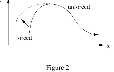
Paradoxically, dynamics can help in achieving some specific control tasks, as well as

hindering others. If the desired system trajectory happens to be one requiring little control input,

then we just have to ensure the initial conditions are good, and make small adjustments during the

trajectory. We are 'riding the system' rather than fighting it. If the initial conditions are bad, then

some initial substantial effort may be required, but after that it is back to small adjustments. Fig 2

illustrates this effect in a general parameter space, {x,y} that might represent position for example.

Figure 2

A simple example is making an object accelerate downwards. We just have to let the object fall

under gravity. Another example is walking. Our legs swing like pendulums, with adjustments so

that we don't trip.

Dynamics can also help by reducing control 'noise'. Since it is the integration of force over

time that is important for causing changes is velocity, short inadvertent spikes of force have a

minimal effect on the trajectory. See Fig 3.

forced

unforced y

x

force

time time

force

3 Perceptual Dynamics in Acoustic Instruments

Acoustic instruments have there own rich dynamics, which are again the result of the Newton's

Laws acting in complicated ways with electric and gravitational forces. Instrument dynamics cover

a broad frequency range. At the top of the range are the audio frequencies. A pure note is a

perceptually static object despite the rapid pressure oscillations, so it is important to differentiate

between the physical dynamics that may yield high frequencies and the perceptual dynamics of

quantities that can be perceived to vary. Such quantities are usually subdivided into pitch, volume

and timbre. The latter is, of course, a catch-all for anything that is not pitch or volume. Depending

on the details of the quantity perceived, the frequency range available for perceived dynamics

extends up to around 50Hz. At higher frequencies we can no longer capture the contour of the

varying quantity and a transition to a new static perception occurs. A common expression used to

describe acoustic instruments is 'liveliness'. This is an almost subconscious reference to perceptual

dynamics. Just as dynamics enriches the recreational activities of the previous section, so it does to

acoustic instruments.

The overall dynamic behaviour of an instrument can be broken down into two main stages;

the dynamics of the interface and the acoustic dynamics of pressure and tension waves, shown in

Fig 4.

Figure 4

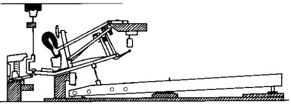
The piano action provides a good example of interface dynamics. The inertia of the hammer and

the escape mechanism combine to create the 'feel' of the keyboard, see Fig 5.

interface dynamics

Figure 5

This dynamics has several subtle consequences. It allows the player to create a wide variety of

strike velocities from small finger movements, since the final velocity is proportional to the impulse

applied by the finger. This is the area under the finger force / time graph shown in Fig 6.

Figure 6

Timing is improved by virtue of the denoising effecting discussed in the previous section. Fast

repeats are possible because the hammer does not return immediately, and can restart a hit from a

short distance away from the string. Because the dynamics of the interface are relatively slow, they

are perceptually relevant.

Acoustic dynamics yields frequencies well above the perceptual range, but also within the

perceptual range. The following list attempts to seperate out different aspects of acoustic dynamics,

but it is by no means exhaustive, and the boundaries are often unclear.

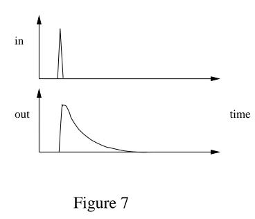
Decay dynamics

Perhaps the simplest examples of dynamics are the volume decays of struck instruments, see Fig 7.

Figure 7

As the different frequency components decay at different rates so the spectral contour and timbre

change during the decay also. Decay dynamics also apply in continuously controlled instruments,

immediately following a period of control, for example when a bow leaves a string.

Beating and related dynamics

Even signals that contain only frequencies above the perceptual upper limit, in the pure spectral

domain, can evoke perceived frequencies. A simple example is the beating of two similar

frequencies. In the sound of a piano note a host of complex timbral dynamics can be heard,

resulting from beating and sympathetic interactions between strings.

Onset dynamics

in

Instruments with which the player interacts continuously for the duration of the note expose richer

dynamics than event based instruments such as percussion. In the continuous case the onset of a

note is a critical period, as the instrument progresses through a turbulent dynamical transition to a

'steady state' oscillation. During the transition the player must respond quickly to the available

indicators of instrument state, the sound and vibration history, in order to guide the instrument to

the desired state. The brevity of the period makes the task all the more challenging.

Locking

The instrument can enter different states that will have a lasting effect on the subsequent note,

independent of the way the input develops. This is a general property of nonlinear dynamical

systems called Mode-locking. An example is register shifting, whereby the output frequency of an

instrument flips by an interval and remains locked into that shift. For instance, overblowing on a

windinstrument can cause an octave rise, which holds as the pressure is reduced. For the most part

locking effects are more subtle than a register change, amounting to a change of timbre.

Evolution Dynamics

During the course of a note played with continuous control, the perceptual features vary smoothly,

but control is still dynamically filtered in subtle ways. For instance, the energy within the

instrument takes time to rise and fall and establish equilibrium as the blowing or bowing strength

changes.

Microunpredictability

in the dynamics of the instrument, as confirmed by the simplified physical models that recreate

these effects.

Macrounpredictability

Many continuously controlled instruments can be driven to state of gross chaotic behaviour

characterized noisy, rapidly fluctuating tones. An example is the vocalized saxophone style in

which vocal sounds interact directly with vibrations in the saxophone. There is a fine line here

between timbre and dynamics.

This section has exposed a variety of physical dynamical effects and challenges that face players of

acoustic instruments. Players learn to achieve these difficult control tasks using the same innate

mechanisms required to deal with everyday dynamics. This is why incorporating physical dynamics

into instruments is a good idea, but one easily overlooked because dynamic control is so much

second nature.

4 Existing Physical Dynamics In Electronic Instruments

Close-coupled physical dynamics has already entered into electronic instrument design in several

ways, as a consequence of emulating acoustic instruments.

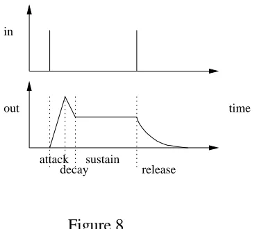
4.1 Dynamic Envelopes

Figure 8

A single event, a key depression, sets the trajectory of a note on course. A key release event makes

the envelope jump towards the release section (To simulate piano dynamics, the sustain section is

removed). This is a simple case because the output only depends on discrete events rather than a

continuum. The envelope is a simple model of keyboard dynamics.

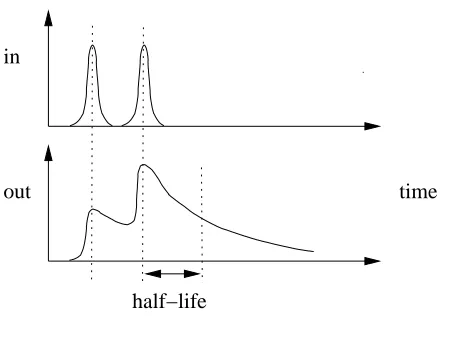
4.2 Effects Processing

Effects processing is a common way of adding dynamical behaviour. It is added at the end of the

signal chain rather than the beginning. A note played into an echo processor for example, produces

a stream of decaying notes. The output at any time depends on previous input events, see Fig 9.

in

time out

decay release

attack sustain

in

The popularity of a range of abstract effects processors is possibly as much due to their dynamical

effect as the immediate timbral effect. While effects offer possibilities for creative design of

dynamics, this is limited by the fact that the effects act at the end of the instrument signal chain

where there are only a few available connections, and not within it, see Fig 10. Also effects

necessarily operate at audio rate, so the computational cost is significant.

Figure 10

4.3 Physical modeling

The advent of physical modeling introduced all the dynamic qualities of acoustic instruments into

the electronic arena. By default, the interface controls connect directly to the synthesizer. The

design process hasn't forced us to acknowledge the importance of dynamics, they have just

appeared as a natural consequence of the modeling process. The 'liveliness' present in acoustic

instruments is inherited.

Physical modeling comes in various forms. Accurate waveguide models seek to simulate

the propagation of sound waves in an object, including critical regions of nonlinear interaction

(Smith, 1992). Matching a waveguide structure to an existing instrument is a demanding task. A

given structure is only capable of a certain range of behaviour. Identifying a structure that will

realize some arbitrary imagined dynamics is intractable in most cases.

Physically inspired modeling models bulk motion in instruments such as shakers, by

making physically reasonable assumptions about the overall sonically relevant behaviour without

worrying about detailed behaviour (Cook, 97). If the bulk dynamics are modeled accurately this

allows the details of interaction sounds to be explored, and is particularly effective when

accompanied by a graphical rendering of the bulk system (Menzies, 99). Fig 11 shows a screenshot

of a system of rigid bodies.

Figure 11

The outer ball can rotate but its centre is fixed, the midsized ball is controlled via an invisible

spring by the mouse. All balls have different resonant properties. It is also possible to model the

acoustic dynamics itself in a semi-physical way, for example using noise for diffuse resonance

(Menzies, 2002)

4.4 Data driven modelling

real instrument. In performance, the output of the clusters mixes short basis samples to generate the

output. Using this approach Schoner has succeeded in producing recognizable, if not hi-fidelity,

string synthesis (Schoner, Cooper, Douglas and Gershenfeld, 1999). This is a promising area for

development, especially if the captured dynamics can be analyzed into perceptually meaningful

'subdynamics', so that they can be creatively transformed.

5 Composing Dynamics

The case for dynamics in instruments has been made. Existing dynamics in electronic instruments

has been reviewed. Now we turn to new practical design processes for adding control processing

dynamics to an interface-synthesis system in which the synthesis component has little or no

inherent perceptual dynamical properties. The following discussion will not assume much technical

knowledge, but hopefully it will also be of interest to the experienced reader by being cast in the

context of instrument control dynamics. Additional background material can be found in

introductory books on filters, for instance (Oppenheim, Schafer and Buck, 1999).

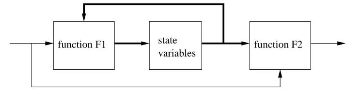
5.1 Linear Filters

the output, and the state variables, are a function of the current input and the state variables, see Fig

12.

Figure 12

Linear dynamical systems, are a subclass with additional properties. They are useful for

modeling a variety of real processes, including physical dynamics, and can be analyzed in depth. In

the language of audio signal processing such systems are more commonly known as linear filters,

and are frequently used as building blocks. In the current context, however, we are interested in

processing control signals rather than audio signals, so the characteristic timescale is larger, and the

bandwidth smaller. A general linear filter can be realized by choosing the state variables to be

recent input and output samples, lagging behind the current sample by fixed amounts. The

functions in Fig 12 are constrained to be linear. If only inputs are chosen then the system is

described as finite impulse response otherwise infinite impulse response. The familiarity of linear

filters will be an aid to their deployment in control processing.

We have already observed that the acoustic dynamics of instruments is often characterized

by non-linearities imbedded within a linear system, so we should question whether non-linearities

should be introduced into the control processing. In this introductory study we shall only consider

linear processing. Interesting results can be hoped from this because the timescale of the processing

is, by design, the same as the human player interacting with it, so the player takes on the role of an

important non-linear interacting element, from the global player-instrument system viewpoint.

state variables

Linear filters can be classified by their order, or how far backwards in time the state

variables extend in their simplified input, output form. Here we consider just first and second order

filters. To aid comprehension, and avoid the technical language of z-transforms, the filters will not

necessarily be constructed in their purest and most efficient form. This doesn't matter because the

computational demands of signal processing at low bandwidth are small compared the demands of

audio rate signal processing in the synthesis section. We shall be more concerned with the details of

the time domain behaviour than would be the case for audio signal processing. Hence filters with

similar frequency responses may have quite different effects as control processors.

5.2 Implementation

There are many ways to implement control filters. Max-related systems have become very popular

for real-time music applications, primarily because of the user-friendly graphical interface. On the

other hand programming languages such as C and C++ offer the greatest flexibility and efficiency.

We shall take the comparatively unpopular middle route of using Csound, which offers several

advantages. Csound is free and available on many platforms, requires modest resources and has a

common multichannel audio interface. The script language is flexible enough to build filter

structures compactly, and enables rapid development. It also means that specific code can be

quoted within this document. One minor draw back is that the real-time capability has been grafted

on to a batch style architecture, so workarounds are sometimes required.

In theory it would be convenient to use the built-in audio filters for control processing.

Unfortunately it is usually found that the filters don't function correctly, if at all, at the low

Depending on what we wish to do, it may be worth upsampling the processed control signal

to improve the final audio output quality. For instance, if a control has a large effect on output

amplitude then up-sampling will reduce zipper noise. Frequency stepping is less noticeable, but

may be worth improving by upsampling.

5.3 A Control Dynamics Kit

The aim here is to present a collection of practical techniques for dynamic control processing. It is

in no way designed to be exhaustive, but rather illustrative of the methods involved. In the

following code snippets, global variables are used so that values can be passed between

instruments, and so that values are retained between performance passes.

is the control time

step, and should be set to

, the inverse of the control sampling rate. The code should reside in a

Csound instr that is active for the duration of the performance, which normally means switching on

from within the score. Time responses to various signals are used to illustrate the dynamics.

1

order Differentiator

This is the simplest useful linear filter for control processing. It outputs the rate of change of the

input, see Fig 13.

in

It has the special property of being point-local. Local means that the output only depends on a

finite stretch of input history. This is true in general for finite impulse response filters. Point-local

additionally means that the history dependence is confined to a small fixed number of samples.

The Csound implementation looks like:

gkout = (gkin - gkinold) * kr

gkinold = gkin

The differentiator is useful for calculating the velocity of an interface object such as a bow or

hammer. From this we can infer the energy associated with interactions of the control object.

Because it is point-local its dynamic behaviour is simple. The acceleration can be found by

chaining two differentiators together.

1

order Integrator

The integrator is the inverse to the differentiator, see Fig 14.

Figure 14

2 _{For the more mathematically inclined: The entire history of an infinitely differentiable function is defined by the} derivatives at a point. In the discrete domain, however, calculating the analog of derivatives amounts to knowing the history, so point-local is useful for describing filters with history dependence that shrinks with time step size.

in

Combining them leaves the input unchanged. The integrator is not local, since it is an infinite

impulse response filter. The output depends on the entire history of input. In the following

implementation our state variable

is a delayed output (

could be dropped and

replaced with

providing it is not modifed later on in the code).

gkout1 = gkout

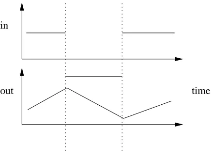
Leaky integrator

In practice the pure integrator is limited in usefulness because the output always grows for positive

input. The leaky integrator is an integrator with an exponential 'drain' added so that the output

decays if no input is present, see Fig 15.

Figure 15

This can model the energy in a resonant object like a string. Energy can be accumulated by

repeated bowing, but ultimately it dissipates.

gkout = (gkin * gkdt) + gkoutold

gkoutold = gkout * gkdecay

Where

and

is the half life of the decay. Note

is not

in

time out

specified as a variable, so that it can be controlled in run time.

1

order Lowpass

We now consider some common filters in their original forms as audio filters. The low pass filter

reduces high frequency content while the lowest frequency content is unchanged, and in fact is the

same as a leaky integrator, but with gain normalized for low frequencies, and a different control

viewpoint (The pure integrator is the low frequency limit of lowpass, with infinite gain at 0Hz). Its

audio implementation in Csound is tone.

gkout = gka * gkin + gkb * gkout1

gkout1 = gkout

For normalization

.

can be controlled directly, or via its relation to the

formal cutoff frequency

kb = 2 - cos(kf*6.282*gkdt)

gkb = kb - sqrt(kb*kb-1.0)

This definition for

is of limited use because the cutoff is not very sharp, but it does at least

provide a way to scale

for differing

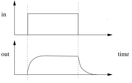
Lowpass intuitively resists change in the input signal, so it provides a simple model for a

physical damping action, see Fig 16.

Figure 16

in

A more accurate model of damping must introduce the notion of acceleration and requires a second

order filter. This is expressed in the resonators below. Lowpass filters can be chained to create

sharper cutoffs, but more ideal filters can be created using other higher-order designs.

Lowpass can also be viewed as a time averaging of the input, so it extracts the large

timescale motion of the input. For sufficiently small

the output converges to the signal offset,

if that exists.

1

order Highpass

The high pass filter attenuates low frequencies. It transmits rapid change well, see Fig 17.

Figure 17

It can be constructed by subtracting the lowpass output from the input. Add :

gkout = gkin - gkout

(a more efficient construction is possible, but efficiency is not very important at control rates). The

highpass is useful for generating signals from sudden changes in the input.

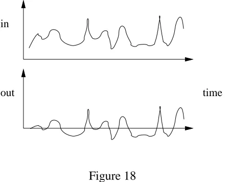
For very low cutoff frequency the highpass is better known as a DC block, which passes all

frequencies unattenuated except the 0Hz or DC offset signal. This is useful for shifting the input so

in

that its time average value is zero, more of a practical than a perceptual-dynamical operation, see

Fig 18.

Figure 18

Resonator

Moving up to second order filters introduces the possibility of oscillation. We consider recursive or

IIR filters whose output depends on the entire history of input, as for the recursive first order filters.

Following the direct form implementation of reson in Csound, we define a control version:

gkout = gkin + ka * gkout1 - kb * gkout2

gkout1 = gkout

gkout2 = gkout1

kca

and

are obtained from the centre frequency

, and bandwidth

as follows:

ka = 4 * kb * cos(kcf * 6.282 * gkdt) / (kb + 1)

Note that numerical errors may cause problems in setting

,

if

is too small compared to kr.

Generally

should be kept to a maximum of 5000, and can be much lower. As the bandwidth is

reduced the filter becomes more resonant and oscillations decay more slowly. Control input which

oscillates near the centre frequency will cause a build up of output oscillations towards a saturation

level, see Fig 19.

in

Figure 19

Resonant-Follower

Resonance can also be approached from a physical viewpoint, and this aids the intuitive

construction of variations on the basic resonator. As an example consider the physical system

shown in Fig 20.

Figure 20

The input control is the position of one end a spring relative to a fixed point. The other end of the

spring is attached to a mass and one end of a damper. The other end of the damper is fixed. The

filter output is the displacement of the mass from its resting position when the input is zero. The

force on the mass depends on the extension/compression of the spring and the velocity of the

damper extension. Without loss of generality take the mass to be 1. In Csound we can integrate the

system to a first approximation with:

in

time out

spring mass damper

gkvel = gkvel + ( (gkin-gkout1)*gkk - gkvel*gkd ) * gkdt

gkout = gkout + gkvel * gkdt

gkout1 = gkout

gkvel

is the velocity,

is the spring constant and

is the damping constant. The step

response is shown in Fig 21.

Figure 21

This is a resonator with DC pass. We call it a resonant-follower to emphasize that the output

follows the input, with added resonance caused by sudden change. It is typical of mechanical

suspension systems that transmit the input but impose resonance and damping as well.

Modified Resonator

The DC component of the resonant-follower can be removed by subtracting the output from the

input. Add:

gkout = gkin - gkout

The step response is shown in Fig 22.

in

Figure 22

This is similar to the resonator step response but with an initial discontinuity. The modified

resonator is equivalent to a resonator and differentiator attached in series, with gain adjustment.

The frequency response does not roll off at high frequencies, so impulses are responded to rapidly

irrespective of the resonant frequency. This feature is exploited in the first example.

Only filters up to 2

order have been considered. This may seem somewhat restrictive, but in

practice a wide range of perceptual dynamics can be approximated well using the filters described.

They have the advantage that the behaviour of each can be clearly understood. Higher order filters

can be built from networks of simpler filters, in a structured way.

6 Example I - Bird

The purpose of the examples is to present complete instruments that use dynamic control

processing, without becoming submerged in synthesis details. To this end we return to the simplest

of instruments, the Theremin, as the starting point. The synthesis section will consist only of a sine

oscillator. The design or compositional elements contributing to the first example are:

a f breath

reed key freq

freq / damping

•

The amplitude and frequency should by effected by output from dynamic control processing.

This should create possibilities for output that the player could not achieve by direct control.

•

The interface is a standard wind controller, such as a Yamaha WX7 / WX11. Use should be

made of the reed pressure sensor.

•

It would be useful if the instrument could be driven to a 'normalized state' where playing keys

produced corresponding scale tones, with no superimposed frequency changes.

•

It would similarly be useful if the instrument could be driven to an 'anti-normalized' state in

which we control the frequency directly and continuously, like the Theremin.

•

The overall aesthetic inspiration is from bird song, the rapid, complex and varied modulation of

simple tones. The effect should be one of intimate rather than loose control, as if the player

were singing directly.

The design process proceeds roughly as follows: To generate frequency modulations, we use a

resonator. But what should drive the resonator? The breath control should be mainly used to control

amplitude, in agreement with the normalization requirement. The staccato nature of bird song

suggests that changes of breath should excite resonant modulation. Using the derived resonator

from the last section we can additionally drive the instrument into an anti-normalized state at low

frequencies, so that breath changes directly control frequency. The remaining piece of the jigsaw is

to use the reed pressure to control the resonant frequency and damping.

Fig 23 shows the overall scheme. The method for controlling the resonant frequency and the

damping is to multiply the time step

by a factor depending on the reed pressure. A tighter

Figure 23

With a tight reed, oscillations die away fast and scales can be played. With a looser reed the

oscillations become slower, and the player interacts dynamically with the oscillations. It is here that

interesting and perceptually unpredictable behaviour can occur. The player has control of the

overall shape of a phrase, but the details of modulation are ever fluid. With a loose reed, breath

drives the frequency directly. By moving rapidly through these regimes the player can achieve a

variety of interesting bird-like performances, that would be impossible without dynamic

processing.

Interesting variations on bird have been made by combining several sine oscillators, each

controlled by slightly different dynamics. The oscillators tend to join and spread according to the

playing conditions, creating chorus like effects and adding more dynamic interest.

7 Example II - Spiro

For the second example we stay with sine modulation, but use a keyboard as the interface. Instead

of using linear filters for dynamic processing we return to the ADSR envelope and wavetable

oscillator, to demonstrate how ‘off the shelf parts’ can be given a new lease of dynamics life. The

ADSR was designed for modeling the volume and filter dynamics of event-based notes. However,

a

f breath

reed

key freq

freq / damping

it also provides a compact dynamical unit for building more general dynamic processing. The

specific criteria this time are:

•

The inspiration is taken from the sustained animal song common in jungles and elsewhere, for

instance by birds and frogs. Cyclic patterns of sound that repeat approximately but never

perfectly.

•

Each key 'contributes' to the output in a different way, and the contribution has dynamical

behaviour.

•

The modulation and pitch wheels can additionally be used to modify the behaviour in some

global way.

These goals are achieved by associating two enveloped oscillators, operating at frequencies in the

perceptual-dynamic range, with each key that has been pressed, one for amplitude and one for

frequency, see Fig 24.

Figure 24

a

f ADSR

The output of the currently active enveloped oscillators is summed to provide the final pitch and

amplitude modulation parameters. Various parameters for the enveloped oscillators, wavetable,

frequency, mode (cycle/oneshot), attack time, decay time, sensitivity to key velocity, are all

selected from tables indexed by the key number. The mod wheel is used to shift the global

oscillator frequencies, while the pitch wheel shifts the final modulation pitch. A simple variation

employs separate amplitude oscillators for right and left channels, so that panning movement

patterns additionally occur.

Csound provides a very efficient structure for implementing this design. A single instrument

definition is accessed by each key that is played, and global variables are used to accumulate the

final modulation parameters (Menzies, 1996). The envelopes are implemented with linenr, which

forces the instrument to remain active after the key is released. This permits a smooth fade of the

effect associated with the key, under the players control.

A variety of tables were generated for experimentation. The most rewarding frequency

range to operate the instrument is just at the point where the patterns of pitches cannot each be

followed exactly but are none the less recognizable from one another. One then perceives a mixture

of dynamics in the sound, possibly resulting from correlations between repeating features. The

effect is analagous to spirograph pattern generators used on some bank notes. As the envelopes

vary the oscillator outputs, so they interact dynamically to create transitional pattern changes in the

output, similar to those heard in nature. A piece, lifeforms, was written combining performances on

bird and spiro, (Menzies, 1996), and has been diffused by the group nerve8 on several occasions.

Conclusion

The motivation for this work has been the belief in the value of dynamical behaviour in

dynamics is important generally, and specifically in the performance of acoustic instruments.

Physical modeling has opened the doors to dynamics, but within certain boundaries. By explicitly

designing perceptually relevant dynamics, a broader more abstract design space is accessible, yet

one still benefiting from dynamics. From a practical viewpoint, the computational costs of

perceptual dynamics are small compared to audio signal processing because of the lower

bandwidth.

Some examples have been given of simple control dynamics processing that yield

compelling results given their simplicity. More generally any dynamical process, whatever its form

or origin, can be considered and transferred to the perceptual band, thus creating a rich field for

experimentation. Of course, the sine generators can be replaced with arbitrarily complex synthesis

units with parameters effecting timbre in many ways. Even physical synthesis units may benefit

from dynamic control preprocessing, by enhancing and modifying aspects of the existing dynamics

that might otherwise be difficult.

Instrument design is foremost an artistic compositional process, but one that is likely to

benefit increasingly from technical proficiency in the abstract manipulation of dynamical systems.

References

Bhushan, N. and Shadmehr, R. 1998. Evidence for learning of a forward dynamic model in human

adaptive control. Journal of Cognitive Neuroscience 5(1), 56--78.

Chadabe, J. 2002. The Limitations of Mapping as a Structural Descriptive in Electronic

Cook, P.R. 1997. Physically Inspired Sonic Modeling (PhISM): Synthesis of Percussive Sounds.

Computer Music Journal, 21(3).

Garnett, G. and Goudeseune, C. 1999. Performance Factors in Control of High-Dimensional

Spaces. Proceedings of the International Computer Music Conference, San Francisco.

Gershenfeld, N. Schoner, B. and Metois, E. 1999. Cluster-Weighted-Modeling for Time Series

Analysis. NATURE, Vol. 397, P. 329-332.

Hilborn, R.C. 2000. Chaos and Nonlinear Dynamics: An Introduction for Scientists and Engineers.

Oxford University Press.

Hunt, A. and Wanderley, M. M. and Kirk, R. 2000. Towards a Model for Instrumental Mapping in

Expert Musical Interaction. Proceedings of the 2000 International Computer Music Conference.

Lennie, P. 1981. The physiological basis of variations in visual latency. Vision Research 21.

Menzies, D. 1995. An Investigation into the Design of Musical Performance Instruments. MSc

report. www.zenprobe.com/dylan/pubs.

Menzies, D. 1995. Bird Csound Instrument code and examples. www.zenprobe.com/os

Menzies, D. 1996. Spiro Csound Instrument code and examples. www.zenprobe.com/os

Menzies, D. 1999. New Performance Instruments for Electroacoustic Music. DPhil thesis.

www.zenprobe.com/dylan/pubs.

Menzies, D. 1999. Physical audio library demos. www.zenprobe.com/dylan/work.

Menzies, D. 2002. Perceptual Resonators For Interactive Worlds. AES 22

International

Conference on Virtual, Synthetic and Entertainment Audio, Helsinki.

Oppenheim, R. W. Schafer, A.V. Buck, J.R. 1999. Discrete-Time Signal Processing (2nd Edition).

Prentice Hall.

Schoner, B. Cooper, C. Douglas, C. and Gershenfeld, N. 1999. Data-driven Modeling of Acoustical

Instruments. Journal for New Music Research, Vol 28(2), 1999.

Smith, J. 1992. Physical modelling using digital waveguides. Computer Music Journal, 16(4):74–

87.