A new method to predict the
aggregate roughness of vegetation
patterns on floodplains
Master Thesis of: M.B.A. ter Haar
Water Engineering & Management University of Twente
Supervisors:
Dr. Ir. J.S. Ribberink
Water Engineering & Management University of Twente
Dr. F. Huthoff
Water Engineering & Management University of Twente
A new method to predict the
aggregate roughness of vegetation
patterns on floodplains
i
SUMMARY
Nowadays rivers are given more room in order to lower the water levels in situations with high discharges. These spaces, called floodplains, are not all year covered with water and thus vegetation will grow on these floodplains. The variety of vegetation is large and different types of vegetation occur on one floodplain. In protecting the land against a possible flood hydraulic model computations play an important role. To be able to do this in an accurate way the characteristics of the river have to be implemented, which also includes the vegetation on a floodplain. This vegetation is modeled as a resistance to the flow.
Due to computational limitations not all small details that describe the river characteristics can be taken into account in the model, for example the roughness patterns. Therefore weighting methods are used to convert multiple roughness values in one cell to one aggregate roughness value that covers the variation in roughness. Currently, the WA-method is the weighting method that is used in the model WAQUA when more than one roughness value is implemented in one grid cell. This method is based on a small number of WAQUA calculations with different roughness patterns. This method predicts an aggregate value independent of the pattern layout and is therefore not always very accurate in predicting the aggregate roughness. The aim of this research is to investigate whether it is possible to create an improved method that takes pattern characteristics into account.
A large series of model calculations with the two dimensional model program WAQUA are carried out to investigate which flow and roughness pattern parameters influence the aggregate roughness of the pattern. WAQUA is a two dimensional model program used for simulation of water movement and transport processes in shallow water and it is based on a vertically averaged approach of the flow field. Different situations are used in the model calculations where the pattern layout, water depth and grid size are varied.
The vegetation pattern layout can be subdivided into parallel oriented patterns, serial oriented and a pattern with multiple square patches (2, 4 and 9) spread over the area. These patterns can be distinguished from each other by the streamlining of the pattern. A parallel pattern has a high streamlining in the flow, followed by the patterns with patches and a serial pattern has a very low streamlining. Furthermore different coverings of rough vegetation on the area are used in the investigation.
The results of these model runs are the aggregate Chézy values that represent the overall flow field. It turns out that the relative serial or parallel direction has a large influence on the aggregate roughness. This can be explained by the existence of flow adaptation processes due to the smooth to rough vegetation transitions. These processes can be divided into two parts: i) a mixing layer along smooth-rough transitions parallel to the flow and ii) flow adaptation behind a smooth-rough patch due to transitions perpendicular to the flow direction. These processes induce an additional roughness on the area, apart from the different roughness of the vegetation. The influences of these mixing layers and adaptation lengths can be expressed as a correction on the aggregate Chézy value. This correction is based on the geometrical lay out of the vegetation pattern.
ii
In order to be able to determine a new prediction method the relations that were found in the results of the model calculations between parameters and aggregate Chézy values are used. The basic principle of the new prediction model is that the parallel function gives an over prediction of the aggregate Chézy value for all pattern types. This already existing parallel function calculates the aggregate Chézy value for situations where the smooth and rough vegetations are parallel oriented in flow direction over the whole area. There is thus an additional roughness that needs to be incorporated in order to reduce the aggregate Chézy value. It is assumed that the mixing layer and the adaptation of the flow are responsible for this additional roughness. These two flow adaptation processes can be expressed as a surface ratio relative to the total area and are the important parameters in the new prediction method. First the parallel patterns are used in order to incorporate the influence of the mixing layers on the area. These pattern types are used for this because in this situation no adaptation of the flow is present and thus the only factor inducing the additional roughness is the mixing layer. When the number of mixing layers is known the additional roughness induced by the mixing layer can be calculated. Next, the additional roughness induced by the adaptation of the flow is determined in the same manner, but this time the vegetation pattern with two patches serial directed was used. This length however is dependent on the width of the rough patch and will thus vary per patch size.
The additional roughness is thus made up of two contributions: i) the influence of the mixing layer, which is expressed as the ratio between the total mixing layer width and the width of the rough vegetation area and ii) the ratio between the free space behind a rough patch and the length of the rough patch. If the adaptation length fits between patches then the adaptation length is used in terms of the free space.
iii
PREFACE
After finishing the bachelor Civil Engineering and Management at the University of Twente, I decided to start with the master course Water Engineering and Management. This thesis forms the completion of my master course at the University of Twente. My research describes a derivation of a new method to predict the aggregate roughness of vegetation patterns on floodplains.
Finishing this thesis would not be possible without the help of my supervisors. Therefore I would like to thank Jan Ribberink and Freek Huthoff for their help and time. During our meetings they gave me constructive feedback and suggestions. Also I would like to thank Jan and Freek for always having time to help me out with my problems.
I also thank my roommates of the graduation room and the employees of the WEM department for the social activities and lunches which were a welcome break from all the hard work. I enjoyed spending my time in the graduation room and the group activities we had, especially the barbeque and the hot potting.
Further I would like to thank my family, friends and especially Bob for all the evening and weekend breaks which were a welcome variation from work.
Marloes ter Haar
v
CONTENTS
SUMMARY ... I
PREFACE ... III
CONTENTS ... V
LIST OF FIGURES AND TABLES ... VII
LIST OF FIGURES... VII
LIST OF TABLES ... IX
1 INTRODUCTION ...1
1.1 BACKGROUND ...1
1.2 FLOODPLAIN ...1
1.3 MODELING VEGETATION ...2
1.3.1Weighted k summation method ...3
1.3.2Weighted average method ...5
1.4 PROBLEM ANALYSIS ...5
1.5 RESEARCH OBJECTIVE AND QUESTIONS ...7
1.6 APPROACH ...7
1.7 OUTLINE OF THE REPORT ...8
2 SHALLOW WATER FLOW MODELING ...9
2.1 GENERAL...9
2.2 SHALLOW WATER EQUATIONS ...9
2.3 GRID ...10
2.4 BOUNDARIES ...11
2.5 EDDY VISCOSITY ...11
3 FLOW ADJUSTMENT PROCESSES ...13
3.1 MIXING LAYER ...13
3.1.1Eddy viscosity ...14
3.1.2Water depth ...16
3.2 ADAPTATION LENGTH ...17
3.2.1Eddy viscosity ...17
3.2.2Water depth and width of rough vegetation ...19
3.3 SERIAL IMPACT ...21
4 WAQUA COMPUTATIONS ...23
4.1 DETERMINING AGGREGATE CHEZY VALUE ...23
4.2 SET UP ...23
vi
4.2.2Parameters of investigation ...24
4.3 RESULTS OVERALL HYDRAULIC ROUGHNESS ...29
4.3.1Water depth ...29
4.3.2Grid size ...30
4.3.3Patterns and coverage ...31
4.3.4Lay out direction ...35
4.4 COMPARISON WITH WA-METHOD ...36
5 A NEW PREDICTION METHOD ...39
5.1 DERIVATION ...39
5.1.1Additional roughness: mixing layer width ...40
5.1.2Additional roughness: flow adaptation behind rough patch ...43
5.1.3Including all pattern types...45
5.2 COMPARISON WITH WA-METHOD ...48
5.3 BEHAVIOUR OF THE MODEL ...49
5.4 BROADER APPLICATION ...51
5.4.1Different patterns ...51
5.4.2Eddy viscosity ...52
5.4.3Roughness ratio ...53
6 DISCUSSION ...55
6.1 MODELING LIMITATIONS ...55
6.2 MODELING CHOICES AND ASSUMPTIONS ...55
7 CONCLUSIONS AND RECOMMENDATIONS...57
7.1 ANSWERS TO RESEARCH QUESTIONS ...57
7.2 RECOMMENDATIONS ...59
8 REFERENCES...61
vii
LIST OF FIGURES AND TABLES
LIST OF FIGUR ES
FIGURE 1:CROSS SECTION OF A RIVER WITH A FLOODPLAIN (TOP: LOW DISCHARGE; BOTTOM: HIGH DISCHARGE). 2 FIGURE 2:ZOOM IN OF AN ECOTYPE MAP OF THE RIVER WAAL AT NIJMEGEN AND BEUNINGEN (RIJKSWATERSTAAT,2010B). 2
FIGURE 3:PARALLEL AND SERIAL FLOW DIRECTION (VAN VELZEN &KLAASSEN,1999) 3
FIGURE 4:RESEARCH MODEL 8
FIGURE 5:LAYER OF WATER IS WATER DEPTH PLUS WATER ELEVATION 10
FIGURE 6:DEFAULT COMPUTATIONAL GRID WITH ARBITRARY OPENINGS 11
FIGURE 7:REPRESENTATION OF THE MIXING WIDTH WHEN THERE IS A TRANSITION FROM SMOOTH TO ROUGH TO SMOOTH. 13 FIGURE 8:ON THE TOP LEFT THE PARALLEL PATTERN IS INCLUDED.THE OTHER THREE FIGURES ARE THE FLOW VELOCITIES [M/S] FOR SITUATIONS WITH AN
EDDY VISCOSITY OF 0.5,5 AND 10 M2/S. 15
FIGURE 9:THE MIXING WITH PLOTTED AGAINST THE EDDY VISCOSITY VALUE. 15
FIGURE 10:ON THE TOP LEFT THE PARALLEL PATTERN IS INCLUDED.THE OTHER THREE FIGURES ARE THE FLOW VELOCITIES [M/S] FOR SITUATIONS WITH
WATER DEPTHS OF 3,5 AND 7 M. 16
FIGURE 11:THE TOP LEFT FIGURE GIVES A ZOOM IN ON THE PATTERN.THE OTHER THREE FIGURES SHOW A ZOOM IN OF THE AREA SHOWING THE FLOW VELOCITIES [M/S] FOR SITUATIONS WITH AN EDDY VISCOSITY OF 0.5,5 AND 10 M2/S. 18
FIGURE 12:THE ADAPTATION LENGTH PLOTTED AGAINST THE EDDY VISCOSITY VALUE. 19
FIGURE 13:THE RESULTS OF THE ADAPTATION LENGTH PLOTTED AGAINST THE WIDTH OF THE ROUGH PATCH FOR THE DIFFERENT WATER DEPTHS. 20 FIGURE 14:THE MEASURED (SOLID LINE) AND THE PREDICTED (DOTTED LINE) ADAPTATION LENGTHS PLOTTED AGAINST THE PATCH WIDTH FOR DIFFERENT
WATER DEPTHS. 21
FIGURE 15:THE WATER DEPTHS IN FLOW DIRECTION, THE GREY DOTTED LINES INDICATE THE STARTING AND END POINT OF THE ROUGH VEGETATION. 22
FIGURE 16:CROSS SECTION OF THE AREA 24
FIGURE 17:CHÉZY VALUE FOR GRASS AND BUSHES FOR VARYING WATER DEPTHS 25
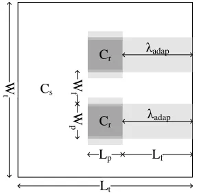
FIGURE 18:FROM LEFT TO RIGHT: TWO PATCHES SERIAL ORIENTED; TWO PATCHES PARALLEL ORIENTED; FOUR PATCHES; NINE PATCHES. 27 FIGURE 19:EXAMPLES OF THE PATTERN LAYOUTS WHERE THE LFBETWEEN IS VARIED PER SITUATION BASED ON THE ΛADAP. 28
FIGURE 20:THE AGGREGATE CHÉZY VALUES OF ALL THE PATTERN TYPES PLOTTED PER WATER DEPTH.FROM LEFT TO RIGHT:3 M,5 M AND 7 M. 30
FIGURE 21:COMPARISON BETWEEN THE RESULTS USING 10 M GRID AND 20 M GRID SIZE 31
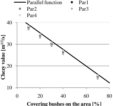
FIGURE 22:THE AGGREGATE CHÉZY VALUES ON AN AREA WITH A PARALLEL PATTERN PLOTTED AGAINST THE COVERING OF BUSHES.THE PATTERN
BELONGING TO PAR1,PAR2 ETC CAN BE FOUND IN APPENDIX V. 32
FIGURE 23:THE AGGREGATE CHÉZY VALUES PLOTTED AGAINST THE NUMBER OF MIXING LAYERS (NΔ). 32
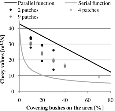
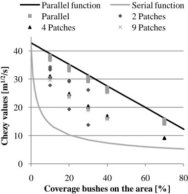
FIGURE 24:AGGREGATE CHÉZY VALUES OF PATTERNS WITH PATCHES PLOTTED WITH THE PARALLEL AND SERIAL FUNCTION. 33 FIGURE 25:THE AGGREGATE CHÉZY VALUES OBTAINED USING A LARGE MODELING AREA PLOTTED AGAINST THE RATIO LFBETWEEN/Λ ADAP.DIFFERENT PATCH
SIZES ARE USED. 34
FIGURE 26:AGGREGATE CHÉZY VALUES OF SERIAL PATTERNS PLOTTED TOGETHER WITH THE SERIAL FUNCTION 35 FIGURE 27:AGGREGATE CHÉZY VALUES OF ALL THE PATTERNS DISCUSSED IN THIS PARAGRAPH PLOTTED AGAINST THE RATIO ∑LP/∑WP WHICH IS THE
DEGREE OF STREAMLINING OF PATTERNS. 35
FIGURE 28:PARALLEL PATTERN WITH DIMENSIONS FOR 10 AND 70 PERCENT COVERING OF ROUGH VEGETATION. 36 FIGURE 29:WITH THE WA-METHOD CALCULATED CHÉZY VALUES PLOTTED AGAINST WITH WAQUA MEASURED CHÉZY VALUES.THE SOLID LINE
INDICATES PERFECT AGREEMENT. 37
FIGURE 30:PLOT WITH THE AGGREGATE ROUGHNESS VALUES OBTAINED WITH WAQUA WITH THE SERIAL AND PARALLEL FUNCTIONS. 39
FIGURE 31:PARALLEL PATTERN SHOWING THE PROPERTIES OF THE PATTERN. 41
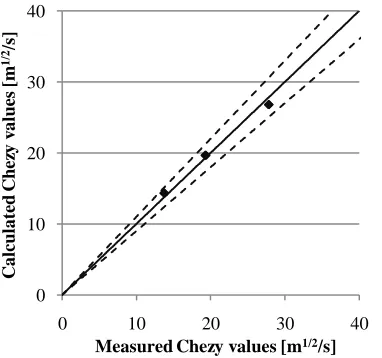
FIGURE 32:CALCULATED CHÉZY VALUES PLOTTED AGAINST THE MEASURED CHÉZY VALUES OF THE PARALLEL PATTERN WITH A WATER DEPTH OF 5M.THE SOLID LINE INDICATES PERFECT AGREEMENT AND THE DOTTED LINES THE 10 PERCENT RANGE. 43 FIGURE 33:PATTERN WITH TWO SERIAL ORIENTED PATCHES.THE PROPERTIES OF THIS PATTERN ARE SHOWN. 43 FIGURE 34:CALCULATED CHÉZY VALUES PLOTTED AGAINST THE MEASURED CHÉZY VALUES OF THE SERIAL ORIENTED PATTERN.THE SOLID LINE INDICATES
viii
FIGURE 35:CALCULATED CHÉZY VALUES PLOTTED AGAINST THE MEASURED CHÉZY VALUES OF ALL THE PATTERNS WITH A WATER DEPTH OF 5M.THE SOLID LINE INDICATES PERFECT AGREEMENT AND THE DOTTED LINES THE 10 PERCENT RANGE. 47 FIGURE 36:COMPARISON OF THE RESULTS OF THE SERIAL PATTERN PREDICTED BY THE NEW MODEL (BLACK POINTS) AND BY THE ALREADY EXISTING SERIAL
FORMULA (GREY POINTS).THE SOLID LINE INDICATES PERFECT AGREEMENT AND THE DOTTED LINES THE 10 PERCENT RANGE. 48 FIGURE 37:COMPARISON OF THE NEW PREDICTION MODEL (BLACK POINTS) AND THE NOW IN USE WA-METHOD (GREY POINTS).THE SOLID LINE
INDICATES PERFECT AGREEMENT AND THE DOTTED LINES THE 10 PERCENT RANGE. 49
FIGURE 38:CHÉZY VALUES BELONGING TO A PARALLEL PATTERN PLOTTED AGAINST THE COVERING OF ROUGH VEGETATION.THE WATER DEPTH,
ROUGHNESS RATIO AND EDDY VISCOSITY VALUE IS VARIED TO INVESTIGATE THE BEHAVIOUR OF THE METHOD. 49 FIGURE 39:CHÉZY VALUES BELONGING TO A PATTERN WITH FOUR SQUARE PATCHES PLOTTED AGAINST THE COVERING OF ROUGH VEGETATION.THE
WATER DEPTH, ROUGHNESS RATIO AND EDDY VISCOSITY VALUE IS VARIED TO INVESTIGATE THE BEHAVIOUR OF THE MODEL. 50 FIGURE 40:COMPARISON OF THE NEW PREDICTION MODEL (BLACK POINTS) AND THE NOW IN USE WA-METHOD (GREY POINTS) FOR OTHER PATTERNS
THAN ARE USED DURING THE DERIVATION OF THE NEW PREDICTION MODEL.THE SOLID LINE INDICATES PERFECT AGREEMENT AND THE DOTTED
LINES THE 10 PERCENT RANGE. 51
FIGURE 41:THE CALCULATED CHÉZY VALUES ARE PLOTTED AGAINST THE MEASURED CHÉZY VALUES WHEN THE EDDY VISCOSITY COEFFICIENT IS 10 M2/S. THE SOLID LINE INDICATES PERFECT AGREEMENT AND THE DOTTED LINES THE 10 PERCENT RANGE. 52 FIGURE 42:COMPARISON OF THE PREDICTION CAPABILITY OF THE NEW MODEL (BLACK DOTS) AND THE WA-METHOD (GREY DOTS) FOR IRREGULAR
PATTERNS CREATED BY VAN VELZEN &KLAASSEN (1999) AND AN EDDY VISCOSITY OF 10 M2/S.THE SOLID LINE INDICATES PERFECT
AGREEMENT AND THE DOTTED LINES THE 10 PERCENT RANGE. 53
FIGURE 43:THE CALCULATED RESULTS PLOTTED AGAINST THE MEASURED RESULTS FOR SITUATIONS WITH A DIFFERENT ROUGHNESS RATIO.THE SOLID LINE INDICATES PERFECT AGREEMENT AND THE DOTTED LINES THE 10 PERCENT RANGE.LEFT FIGURE: Α2 OF 2.62.RIGHT FIGURE: Α2 OF 1.7. 54 FIGURE 44:COMPARISON OF THE PREDICTION CAPABILITY OF THE NEW MODEL (BLACK DOTS) AND THE WA-METHOD (GREY DOTS) FOR PATTERNS
CREATED BY VAN VELZEN &KLAASSEN (1999) AND A DIFFERENT ROUGHNESS RATIO.THE SOLID LINE INDICATES PERFECT AGREEMENT AND THE
DOTTED LINES THE 10 PERCENT RANGE. 54
FIGURE 45:LEFT TOP:24 RANDOMLY PLACED PLOTS WITH 16% COVERAGE, LEFT MIDDLE:5 RANDOMLY PLACED PLOTS WITH 20.8% COVERAGE, LEFT BOTTOM: ONE STRIPE PERPENDICULAR TO THE FLOW DIRECTION WITH 20% COVERING.RIGHT TOP:11 RANDOMLY PLACED PLOTS WITH 16.5%
COVERING, RIGHT MIDDLE: ONE PLOT WITH 16.7% COVERAGE, RIGHT BOTTOM: ONE STRIPE PARALLEL TO THE FLOW DIRECTION WITH 18.75%
COVERAGE (VAN VELZEN &KLAASSEN,1999) 67
FIGURE 46:INFLUENCE PATTERN TREES ON THE CHÉZY VALUE (VAN VELZEN AND KLAASSEN,1999) 69 FIGURE 47:INFLUENCE PATTERN BUSHES ON THE CHÉZY VALUE (VAN VELZEN AND KLAASSEN,1999) 69
FIGURE 48:CONCEPT OF PARALLEL FLOW 71
FIGURE 49:CONCEPT OF SERIAL FLOW 72
FIGURE 50:LAY OUT OF THE PARALLEL PATTERNS. 73
FIGURE 51:CALCULATED CHÉZY VALUES PLOTTED AGAINST THE MEASURED CHÉZY VALUES OF ALL THE PATTERNS WITH A WATER DEPTH OF 3M.THE SOLID LINE INDICATES PERFECT AGREEMENT AND THE DOTTED LINES THE 10 PERCENT RANGE. 83 FIGURE 52:CALCULATED CHÉZY VALUES PLOTTED AGAINST THE MEASURED CHÉZY VALUES OF ALL THE PATTERNS WITH A WATER DEPTH OF 7M.THE
ix
LIST OF TABLES
TABLE 1: RESULTS MODEL RUNS WITH VARYING EDDY VISCOSITY ... 14
TABLE 2:MIXING LAYER WIDTHS BELONGING TO A CERTAIN WATER DEPTH ... 16
TABLE 3:RESULTS IN DISCHARGES FOR MODEL RUNS WITH ONE SQUARE PATCH AND VARYING EDDY VISCOSITY COEFFICIENT. ... 19
TABLE 4:DIMENSIONS IN METERS OF THE SMOOTH SPACE BETWEEN ROUGH PATCHES. ... 27
TABLE 5:DIMENSIONS IN METERS OF THE ROUGH VEGETATION AREAS PER PATTERN TYPE. ... 29
TABLE 6:CHÉZY VALUES FOR GRASS AND BUSHES FOR DIFFERENT WATER DEPTHS. ... 30
1
1
INTRODUCTION
In this chapter an introduction will be given of the problem that is considered in this study. First the background of the study will be shortly explained, in order to give insight in the importance of modeling the characteristics of a river properly. Secondly a short description is given of a floodplain followed by the way in which vegetation on a floodplain is modeled at this moment. After that the problem analysis states what the problems are that are faced when it comes to modeling vegetation. Based on this problem the objective and the research questions are defined and based on these research questions the approach of the study is given. In the final section the outline of the report is presented.
1.1
BACKGROUND
In the last decades the economic growth and the development of urban communities in the Netherlands has resulted in more pressure on free space. To obtain more land for building activities the width of the riverbed has been restricted in order to fulfil the needs. One way to do this is by canalization, by which the river is made more straight and is bounded by dikes. These dikes have been raised during the years in order to keep the area behind the dikes safe against a possible flood. This may result in larger damages after a flood because the water level is higher and the economic value behind the dikes has increased.
Due to climate change the discharge of the rivers will further increase in the future. An option to protect the area within the dikes is to raise the dikes even further, however from a technical point of view this is not an option. Therefore another course has been adopted in the Netherlands: ‘Room for the river’. The trend in this course is to give the river more room to flow in, in order to lower the water levels (Projectorganisatie Ruimte voor de Rivier, 2007).
Different measures can be taken in giving more room to the river. Some of the measures are: lowering the groins, lowering the summer bed, removing obstacles in the floodplain, lowering of the floodplains and widening the floodplain. A great deal of the measures incorporates building or adapting a floodplain, which has to lower the water level. In protecting against a possible flood hydraulic model computations play an important role. The results of the computations are crucial for acceptance or rejection of developments in the river system (Van Velzen et al., 2003). It is thus important to describe the flow over a floodplain accurately in order to design a measure that will lower the water level sufficiently. This modeling can be done with a 2D river model called WAQUA that is used in The Netherlands (Vollebregt et al., 2003 and for some examples see Svašek Hydraulics, 2010).
1.2
FLOODPLAIN
2
Furthermore, by temporary storing more water, the floodplain lowers the water level downstream of that location.
Figure 1: Cross section of a river with a floodplain (top: low discharge; bottom: high discharge).
To get insight in the types of vegetation on a floodplain, maps of ecotypes are used. These charts present the vegetation structure and are obtained from aerial photographs. From these photographs the structure of the different vegetation types are visual distinguished. When interpreting a photo it is not possible to account for every detail on the floodplain. This means that small groups of trees or bushes will not be taken into account in the analysis (Rijkswaterstaat, 2010a & Van Velzen et al., 2003). In figure 2 a part of an ecotype map retrieved from Rijkwaterstaat (2010b) is included from the Waal at Nijmegen and Beuningen in the Netherlands. The land that is shown next to the river represents floodplains. This map shows that different types of vegetation on a floodplain are available for input for model calculations.
Figure 2: Zoom in of an ecotype map of the river Waal at Nijmegen and Beuningen
(Rijkswaterstaat, 2010b).
1.3
MODELING VE GETATION
When a river is modeled the important aspects that can influence the flow in that river needs to be incorporated in the model in order to produce results that are accurate and meaningful. This includes the floodplain, which means that the vegetation on the floodplain needs to be represented in the model input. This vegetation is implemented as a resistance factor in the flow. This resistance is dependent on the height, frontal area, a resistance coefficient and the roughness of the bed (Van Velzen et al., 2003). Different vegetation types will thus induce a different resistance to the flow. Because a variety of vegetation is present on a floodplain, patches with different resistances to the flow are present. This
Summerdike Winterdike
Floodplain
Situation in summer
Summerdike Winterdike
Situation in winter
Grass Wood
3 means that when the floodplain is modeled these varying resistances must be incorporated in the model description.
The resistance due to vegetation is implemented by a roughness parameter. Because it is not possible to account for every detail, grid cells with a certain size are defined. The input in one grid cell needs to be uniform, and thus a roughness variation within the grid cell cannot be represented, and one roughness value is given instead of the pattern. This process of replacing a pattern of roughness values by one roughness value will exclude a degree of accuracy, which is also influenced by the size of the grid cells that is chosen in the model, because the larger the grid cell the higher the chance that there are more vegetation types captured in one cell.
SOBEK and WAQUA are two different flow models that are used in The Netherlands. SOBEK is one dimensional and WAQUA is two dimensional. In SOBEK large cells are used that can represent areas of hundreds of square meters and in WAQUA grid sizes of several square decameters are used (Gao, 2004, RWS-Waterdienst & Deltares 2009a, 2009b) The degree of accuracy that is lost by excluding a roughness pattern is thus also different per flow model that can be used. In order to reduce the inaccuracy, weighting methods weight the pattern of roughness values to one value. In this way the effect of a pattern is captured in one value. In the following sub paragraphs two methods that are designed to do this are explained, first the weighted k summation method and after that the weighted average method which is used in the model WAQUA at this moment.
1.3.1 WEIG H TED K SU MMATIO N ME TH O D
A method to calculate an aggregate Chézy value is presented in Van Velzen & Klaassen (1999). At that time the method ‘weighted k summation method’ (from now on referred to as WKS-method) was used. This method is a variation to the suggested method grid averaging by Van Urk (1983, according to Van Velzen & Klaassen (1999)), in which is recommended to sum the Nikuradse k-values up by area division. It is tried to develop a method to describe the vegetation patterns. For that a distinction is made between serial and parallel flow direction, see figure 3. Van Urk (1983, according to Van Velzen & Klaassen (1999)) concluded that there are large differences between these two types of flow directions. However, it was not possible to point out how the flow resistance due to a patch of trees would be in proportion of the parallel or serial flow situation.
Figure 3: Parallel and serial flow direction (Van Velzen & Klaassen, 1999)
The WKS-method in formula:
[1.1]
With:
kt = Representative k-value of the different vegetation types [m]
kg = Nikuradse value of the basis vegetation [m]
4
kb = Nikuradse value of group(s) of trees/bushes [m]
x = Part of the area covered by trees/bushes [-]
The Chézy value belonging to a certain Nikuradse k-value can be calculated using the following formula (Ribberink & Hulscher, 2008):
[1.2]
With:
C = Chézy value [m1/2/s]
g = Gravitational acceleration [m/s2]
κ = Von Karman constant (0.41) [-]
h = Water depth [m]
kn = Nikuradse value [m]
This WKS-method has two disadvantages; first of all it is never been tested and secondly the influence of grouping of vegetation and the direction to the flow of the vegetation is not taken into account. Van Velzen & Klaassen (1999) tested this method with use of the model program WAQUA and tried to refine this method in order to eliminate these two disadvantages. Three different formulas are deduced, one for parallel flow, one for more spread vegetation and one for one group of trees, these formulas can be found in Appendix I. In the study different patterns were investigated which are characterized by grouping and frontal shape; an aerial view can be found in Appendix II.
The patches in these patterns are covered with rough vegetation and cover approximately twenty percent of the total area. The vegetation roughness of bushes and trees were included as Chézy roughness values of respectively 4.8 m1/2/s and 42.9 m1/2/s and the water depth was kept as constant as
possible at 5 m. The total discharge was the result of the model runs and with this discharge the aggregate Chézy value was calculated using the inverse Chézy formula:
[1.3]
With:
Qwaqua = Discharge [m3/s]
h = Average water depth (5m) [m]
B = Width [m]
∆ h = Difference in height due to the slope [m]
L = Length area [m]
5 covering an equal prediction. The difference in Chézy value between the WKS-line and the result is the deviation of the prediction with the WKS-method for that particular pattern.
1.3.2 WEIG H TED A VERAG E M E T H O D
In Van Velzen et al. (2002) another method is given instead of the WKS-method because with certain vegetation combinations the WKS-method leads to an overestimation of the roughness. The newly proposed method, the weighted average method (from now on referred to as the WA-method), is based on the individual formulas to calculate the Chézy roughness for a serial and a parallel pattern see formulas 1.4 and 1.5 (Ministry of Transport, Public Works and Water Management, 2008). The derivation of these formulas can be found in Appendix IV.
[1.4]
[1.5]
With:
Xi = Area fraction roughness type i [-]
Cri = Chézy value roughness type i [m1/2/s]
Cp = Chézy value for parallel pattern [m1/2/s]
Cs = Chézy value for serial pattern [m1/2/s]
The WA-method used in the model WAQUA when a pattern needs to be converted to a single Chézy value is combined out of these parallel and serial approaches:
[1.6]
With:
Crc = Average Chézy coefficient [m1/2/s]
Cs = Chézy coefficient with serial pattern [m1/2/s]
Cp = Chézy coefficient with parallel pattern [m1/2/s]
φ = Weighting factor [-]
In order to obtain a value for φ , Van Velzen et al. (2002) plotted the line obtained with equation 1.6 in such a way that it went on average as good as possible through the different patterns (1, 2, 3 and 4 as used in Van Velzen & Klaassen, 1999). It turned out that this factor was 0.6. This can be seen in Appendix III where the figures are included. It is also clear from these figures that with a small percentage woods or bushes the Chézy value changes a lot, the gradient is strong, and with a high coverage of rougher vegetation the gradient gets lower.
1.4
PROBLEM AN ALYSIS
6
defined roughness value on the floodplain will result in inaccurate flow properties, such as water level and flow velocity. When a measure has to be designed in order to agree with a certain water level that occurs with a specific return period, these inaccurate results will lead to a measure that is too safe or not safe enough according to the safety requirements.
Van Velzen et al. (2002) stated that the value of 0.6 in the WA-method can only be used when there is a possibility for the flow to redistribute. This means that the flow will follow the route with the lowest resistance and will flow over the areas with a high Chézy roughness value. But no limits are given to point out what is a redistribution of the flow and what not, the range of applicability is thus not very clear. Taking a value of 0.6 for φ means that it is always assumed that sixty percent of the vegetation is oriented serial to the flow direction and forty percent parallel. This is of course not always the case as for example in the patterns that were used in the assessment.
The WA-method is based on a few model runs. In these runs no variation was made in water depth, grid size and vegetation pattern which are all factors that vary from one floodplain to another. These different parameters might have an effect on the combined roughness value in WAQUA because every floodplain is different and the latest developments in airborne laser scanning and spectral remote sensing lead to the development of more precise vegetation maps (Straatsma & Baptist, 2008). When the same grid cell sizes are used as now, but with more precise input information, the WA-method will be used more often to calculate an aggregate roughness value.
Also, experiments revealed that the effective friction factor increases when roughness patterns are present (Van Prooijen, 2004 and Vermaas, 2008). Furthermore in the figures of Van Velzen et al. (2002), in Appendix III, it can be seen that not all the aggregate Chézy values resembling a roughness pattern lay perfectly on the line representing the WA-method, and thus do not correspond to the value that is calculated by the WA-method. A deviation from this WA-method thus means that it will under or overestimate the roughness value. This deviation will eventually lead to a modeled water level in WAQUA that is based on a wrong aggregated roughness value.
If flow over a floodplain is modeled not all the details can be taken into account because of computational limits or the information is not available and if it is available the inclusion of them takes too much time and effort. It is thus necessary to model a floodplain as good as possible with the least input data. A weighing method or some kind of model that can give a good representation of the vegetation pattern is thus needed.
7
1.5
RESEARCH O BJECTIVE AND QUEST IONS
The objective of this study is to get insight in what way patch parameters influence the aggregate roughness of a vegetation pattern and to deduce a method in predicting this aggregate roughness. In order to reach the objective of the study the following question needs to be answered.
How can an improved model for floodplain roughness be developed which incorporates the influence of roughness pattern variation.
The next questions will help to answer the main question:
How can the vegetation pattern be characterized in general parameters that control the aggregate roughness?
How do the water depth and grid size of the model have an influence on the aggregate roughness obtained with the model WAQUA on a floodplain with a pattern of two vegetation types?
What is the deviation of the aggregate roughness value obtained from WAQUA model runs with different patterns of roughness patches compared with the WA-method?
Can an improved roughness prediction method be developed instead of the WA-method by taking into account additional control parameters?
1.6
APPROACH
To achieve the research objectives in paragraph 1.5 the following research approach is used.
The first step is to define different patterns, where geometrical dimensions are considered as characterizations for the vegetation pattern.
When these dimensions are defined the model runs can be made with WAQUA in which the variables water depth and grid size are varied in order to investigate the influence of these variables on the aggregate roughness.
If the results of the model runs are known, an analysis of the aggregate roughness values is made. These values will be compared with the WA-method and ‘serial’ and ‘parallel’ theories and the results of the different patterns are compared with each other in order to find out what the influence of the geometrical dimensions of the pattern is on the aggregate roughness value. Finally it is investigated how a new weighting method can be defined in order to predict the
8
Figure 4: Research model
1.7
OUTLINE OF THE REPORT
In chapter 2 the important aspects for this study of the two dimensional model program WAQUA are presented. Chapter 3 contains the explanation of the flow adaptation processes that take place when there is a smooth to rough transition in bottom roughness. Also the special case of a complete serial pattern, where the total width of the area is covered with rough vegetation, will be shortly explained. After that, in chapter 4, the input description of the model calculations are given and the results of the calculations are presented. The derivation of a new prediction method is given in chapter 5, which is based on the results of the calculations. Chapter 6 gives the discussion and finally, in chapter 7, the conclusions and recommendations of this study are presented.
Vegetation patterns
Different water depths
Different grid sizes
Understanding which parameters influence
the average roughness Insight in the applicability of the weighting methods Predict the average
roughness of a vegetation pattern
before modeling WAQUA
Comparing average Chézy values with
WA-method Comparing average
Chézy values between different
patterns
9
2
SHALLOW WATER FLOW MODELING
The model runs that are performed for this study are executed with WAQUA which is a program part of SIMONA which is provided by Rijkswaterstaat. Not all the features of WAQUA will be explained here, only the features that are important for this study. For a full description see Ministry of Transport, Public Works and Water Management (2008) and Ministry of Transport, Public Works and Water Management (2009b).
2.1
GENERAL
The two-dimensional model program WAQUA is used for simulation of water movement and transport processes in shallow water. It is based in a vertically averaged (two dimensional) approach of the flow field. The system can simulate hydrodynamics in geographical areas which are not
rectangular, and bounded by any combination of closed boundaries (land) and open boundaries (b
of Transport, Public Works and Water Management, 2008). The development started with the work of Leendertse, but the current methods are developed by Stelling in 1983. The model is for example used to schematize the rivers Meuse, Rhine and IJssel for computing the water levels in exceptional circumstances in order to decide on the required height of dikes to reduce the risk of flooding to an acceptable level (Vollebregt et al., 2002).
Rivers with their floodplains are typical examples of shallow water. Flood waves in rivers are often very slowly varying (duration of several days). The propagation speed of flood waves is small, of the same order as the flow velocity. This can be explained by the fact that bottom friction is a dominant effect in this case (Vreugdenhil, 1994).
2.2
SHALLOW WA TER EQ UATI ONS
As discussed above WAQUA is used in flows where the characteristic horizontal length scales (dimensions of the flow domain and wavelength) are much larger than the vertical length scale (water depth). The flows are boundary layer types of flow. Therefore the motion of a fluid particle is mainly horizontal and the accelerations in vertical direction are neglected with respect to the gravity. Thus it is justifiable to neglect the vertical acceleration and advection. Also the vertical component of the Coriolis force and the stress components in the vertical direction may be neglected.
The shallow water equations that are used with a rectangular grid, excluding Coriolis and wind friction, are as follows (Praagman, 2005):
[2.1]
[2.2]
10 With:
u,v = Components of depth mean current [m/s]
ζ = Water elevation above plane of reference (see figure 4) [m] h = Water depth below the plane of reference (see figure 4) [m]
H = h + ζ [m]
g = Acceleration due to gravity [m/s2]
C = Coefficient of Chézy to model bottom [m1/2/s]
ε = Eddy viscosity coefficient [m2/s]
Figure 5: Layer of water is water depth plus water elevation
2.3
GRID
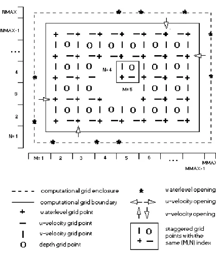
The computational grid that is used in WAQUA is illustrated in figure 6. A grid is laid on the rectangular area, where the square grid space size in meters is chosen, and the number of grid spaces in two dimensions, Nmax and Mmax. Four basic physical properties pertain in each grid space: water level, depth, u-component of velocity and v-component of velocity. During the simulation different time integrals are computed using an ADI staggered time integration method over two half time steps, so not all primary data is available at the same time. At the first half time step the u-velocities and resultant water levels are calculated and also separate v-velocities (explicit). At the second half time step the v-velocities and resultant water levels are calculated together with the separate u-velocities (explicit).
The basis of the WAQUA system is the staggered grid. This implies that the modeling system can be seen as a large number of linked, column shaped, volumes of water. The corners of these volumes are the depth points of the grid. Each volume of water has four sides through which water may flow in or out of the volume (Ministry of Transport, Public Works and Water Management, 2008).
Plane of reference
ζ
11
Figure 6: Default computational grid with arbitrary openings
2.4
BOUNDARIES
At the boundaries of the area information about these boundaries are needed. Two types of boundaries can be distinguished: closed and open boundaries. Closed boundaries are mostly locations that are bounded by land. Open boundaries are boundaries where water is bounded by water.
Open boundaries where river data are given to drive the model are needed. In the case of this study water level boundaries are given in which the water levels are given at the beginning and at the end of the model. In general, the open boundaries feed into the computational grid from just outside. This also implies that the ends of an open boundary do not extend beyond the grid.
2.5
EDDY VISC OSITY
13
3
FLOW ADJUSTMENT PROCESSES
As already discussed in chapter 1, on a floodplain a variety of vegetation is present. This variation creates patches of various vegetation types. When there are patches of rougher vegetation present on an area, there will be transitions in flow velocities, because the water will flow faster above smooth vegetation than above rough vegetation due to the induced resistance. In order to comply with these differences the flow has to adjust itself. These adjustments give rise to processes in the flow around the smooth-rough transitions. These processes induce an additional roughness on the area, on top of the different roughness values of the vegetation. These adjustment processes are handled in this chapter. The adjustments are separated in three parts; i) a mixing layer that is located at the transition parallel to the flow direction, ii) an adaptation length on the lee side of a transition perpendicular to the flow direction and iii) a special situation where it is not possible for the flow to redirect around the rough vegetation, referred to as serial impact. In this chapter these three processes are explained and it is tried to predict the geometrical dimensions of them with use of the model WAQUA.
3.1
MIXING LAYE R
White and Nepf (according to Zong and Nepf, 2010) described the flow structure and exchange at the interface between parallel regions of emergent vegetation in an open-channel. The drag discontinuity at this interface creates a shear layer that in turn generates large coherent vortices. This is also what happens at the interface of smooth and rough vegetation which is called the mixing layer. A larger part of this mixing layer lies above the smooth side than above the rough side (Vermaas, 2008, Van Prooijen, 2004). Figure 7 shows the transition of the velocity from high above the smooth side, to low above the rough bottom and to high again above the smooth side. The mixing width, δ , is the property that influences the aggregate roughness on the area.
Figure 7: Representation of the mixing width when there is a transition from smooth to rough to
smooth.
Van Prooijen (2004) executed experiments in order to gain a better understanding of the mixing layer. From the mean streamwise velocity data the characteristic properties of the downstream development of a shallow mixing layer were determined. These characteristics are: the decrease of the velocity difference, the non-linear widening of the mixing layer and the shift of the mixing layer to the low velocity side.
Smooth Rough
Smooth
δ u
14
Also Vermaas (2008) executed laboratory experiments. The bottom consisted out of a hydraulically rough and smooth section in parallel direction of the flow. Measurements were done for five different depths and discharge settings. Due to the different roughness’s between the sections, the flow decelerates above the rough side and accelerates above the smooth side. When the mixing layer is under development, the flow redistributes, water volume is transferred from the rough to the smooth side. In the developed part of the mixing layer, the bed shear stress above the rough side is higher than at the smooth side. This requires longitudinal momentum to be transported from the smooth to the rough side in order to maintain a mixing layer that is uniform in x-direction.
When a parallel pattern is implemented in WAQUA the mixing layer is constant along the length of the area and it is situated more to the smooth side. The other characteristics that were found with the experiments executed by Van Prooijen and Vermaas are not present in the results of WAQUA. This is because WAQUA is a depth averaged flow model that uses a constant eddy viscosity without modeling turbulence in detail. The eddy viscosity coefficient thus has a large influence on the mixing layer width.
Since all the model runs in this study will be executed with the WAQUA model, first the behaviour of the mixing layer will be shortly studied with some specific model runs. A parallel pattern type is used in order to determine the mixing width. The grid size is 20 m, slope 1 10-4 and the total area 1000 by
1000 m. First the influence of the eddy viscosity coefficient will be studied followed by the water depth to increase the understanding of the important factors that influence the mixing layer in this study.
3.1.1 EDDY VISCO SI TY
To understand what this eddy viscosity terms does model runs were executed where the eddy viscosity is varied. A parallel vegetation pattern is implemented with Wf of 700 m and Wp of 300 m which
means a covering of thirty percent rough vegetation. The water depth at the beginning and end of the area is set at 5 m. In Table 1 the discharge and the aggregate Chézy values can be found.
Eddy viscosity [m2
/s] 0.5 5 10
Discharge [m3
/s] 3442 3319 3246
Chézy [m1/2
/s] 30.8 29.7 29.0
Table 1: results model runs with varying eddy viscosity
15
Figure 8: On the top left the parallel pattern is included. The other three figures are the flow
velocities [m/s] for situations with an eddy viscosity of 0.5, 5 and 10 m2/s.
In figure 9 the mixing width in meters is plotted against the eddy viscosity coefficient. The results are obtained from calculations similar as the situations shown in figure 8. These widths are determined from a parallel pattern with a water depth of 5 m where only the eddy viscosity has been varied; all the other parameters were kept constant. Plots with steps of 0.05 m/s in flow velocity are used to determine the mixing layer width which is assumed to be an accurate representation of the flow field. The form of the relationship between the mixing layer width and the eddy viscosity coefficient, shown in figure 9, indicates that the mixing width and the eddy viscosity have the following dependence:
[3.1]
It can thus be concluded that when the eddy viscosity coefficient is changed in the model WAQUA the mixing layer will vary in width and thus has an influence on the aggregate roughness.
Figure 9: The mixing with plotted against the eddy viscosity value.
Bushes
Wf
Wp
Grass
ε = 0.5 m2 /s
δ
δ ε = 5 m2
/s
δ ε = 10 m2
/s
Velocity [m/s]
0.30 – 0.35
0.85 – 0.90 0.90 – 0.95 0.95 – 1.00 0.80 – 0.85 0.75 – 0.80 0.70 – 0.75 0.65 – 0.70 0.60 – 0.65 0.55 – 0.60 0.50 – 0.55 0.45 – 0.50 0.40 – 0.45 0.35 – 0.40 0.25 – 0.30 0.20 – 0.25 0.15 – 0.20 0.10 – 0.15
0 50 100 150 200 250
0 5 10
M ixi n g w id th [ m ]
16
3.1.2 WATER DEP TH
Also different water depths are used to investigate what the influence is of this parameter; 3, 5 and 7 m (explanation of the choice of these water depths will be given in chapter 4). The same parallel pattern as in paragraph 3.1.1 was used to determine the influence of the eddy viscosity on the mixing layer.
Figure 10: On the top left the parallel pattern is included. The other three figures are the flow
velocities [m/s] for situations with water depths of 3, 5 and 7 m.
Because with a larger water depth a relatively smaller part of the water column is affected by the vegetation, the overall roughness will be smaller. This gives rise to different velocity differences between situations with another water depth. This is because the difference in flow velocity above the smooth and rough side increases with a larger water depth. For a water depth of 3 m the flow velocity of the smooth side is approximately 0.65 m/s and above the rough vegetation side 0.01 m/s which gives a difference of 0.64 m/s. With a water depth of 7 m the flow velocity above the smooth side is 1.2 m/s and above the rough side 0.2 m/s which gives a difference of 1 m/s which is larger than the difference in the 3 m situation.
In table 2 the mixing layer widths per water depth are given. When a different water depth is present in WAQUA the water depth will thus have an influence on the mixing layer width, although small compared to the influence of the eddy viscosity coefficient. This will be taken into account in this study.
h = 3 m h = 5 m h = 7 m
Mixing layer
width [m] 40 40 60
Table 2: Mixing layer widths belonging to a certain water depth
Bushes
Wf
Wp
Grass
h = 3 m
δ
δ h = 5 m
δ h = 7 m
Velocity [m/s]
0.30 – 0.35
0.85 – 0.90 0.90 – 0.95 0.95 – 1.00 0.80 – 0.85 0.75 – 0.80 0.70 – 0.75 0.65 – 0.70 0.60 – 0.65 0.55 – 0.60 0.50 – 0.55 0.45 – 0.50 0.40 – 0.45 0.35 – 0.40 0.25 – 0.30 0.20 – 0.25 0.15 – 0.20 0.10 – 0.15 0.05 – 0.10 0.00 – 0.05
17
3.2
ADAPTATION LENGTH
After a rough patch, the flow will experience a smoother roughness and will thus gradually increase flow velocity. The distance that the flow needs to recover from the disturbance in the flow is the adaptation length. An indication of Sieben (2006) is that with a shallow water flow the length scale is more than 20 to 50 times the water depth. Taking a water depth of 5 m means that the length scale ranges from 100 till 250 m.
Labeur (1998) gives a description of how long the distance is that is needed for the flow to adapt to the new situation after a sand pit. This adaptation length is corrected for very wide sand pits, with the following formula:
[3.2]
With:
[3.3]
λ = Adaptation length [m]
λ’ = Adapted adaptation length to width of the pit [m]
β = Equivalent width [m]
B = Width of the sand pit [m]
h = Water depth [m]
C = Chézy coefficient [m1/2/s]
g = Acceleration due to gravity [m/s2]
The equivalent width value has not been deduced in Labeur (1998), but with an increasing value the adaptation length increases. It is shortly investigated whether this relation can also be used in the case of vegetation patches.
It is expected that the water depth has an influence on the adaptation length of the flow. Also the influence of the eddy viscosity value on the flow adaptation length is shortly investigated. With the use of some model runs with WAQUA the influence of these two parameters on the adaptation length is investigated. A large area, 4 by 4 km is used in order to capture the complete adaptation length. Square patches of rough vegetation (bushes) are implemented with varying patch size to investigate the influence of the width of the patch on the adaptation length. In the following paragraphs the influence of the parameters are investigated.
3.2.1 EDDY VISCO SI TY
18
term is larger, the mixing layer is wider (see paragraph 3.1.1) and thus the width that is felt by the flow is larger with a higher eddy viscosity value.
The flow velocities above the patch are increasing with higher eddy viscosity values. The differences in flow velocities above the rough area and above the smooth area decrease with increasing eddy viscosity value. The adaptation of the flow thus needs a smaller length to adapt to the new flow situation above the smooth area; this can explain the minor decrease in adaptation length with increasing eddy viscosity coefficient.
Figure 11: The top left figure gives a zoom in on the pattern. The other three figures show a zoom
in of the area showing the flow velocities [m/s] for situations with an eddy viscosity of 0.5, 5 and 10
m2/s.
The adaptation length is obtained from figures given in figure 11 with a velocity step of 0.05 m/s which is assumed to be a reasonable accurate representation. The length that is needed to reach half the flow velocity belonging to a smooth situation is assumed to be half of the total adaptation length. Obtaining the adaptation lengths for the different situations with varying eddy viscosity coefficients gives the relation shown in figure 12. This figure also shows the decreasing adaptation length with increasing eddy viscosity.
Grass
Velocity [m/s]
0.30 – 0.35
0.85 – 0.90 0.90 – 0.95 0.95 – 1.00 0.80 – 0.85 0.75 – 0.80 0.70 – 0.75 0.65 – 0.70 0.60 – 0.65 0.55 – 0.60 0.50 – 0.55 0.45 – 0.50 0.40 – 0.45 0.35 – 0.40 0.25 – 0.30 0.20 – 0.25 0.15 – 0.20 0.10 – 0.15
1.00 – 1.05 1.05 – 1.10 1.10 – 1.15 1.15 – 1.20
ε = 0.5 m2
/s
ε = 5 m2
/s ε = 10 m2/s
19
Figure 12: The adaptation length plotted against the eddy viscosity value.
Whether the influence of the eddy viscosity on the adaptation length will also affect the aggregate roughness of the area cannot be said for certain based on the above findings. Although the length decreases with an increasing eddy viscosity value the width increases and thus the total effect might be minor. Therefore the discharges of the total areas are given in table 3. This table shows that the discharges are almost equal and thus the influence of the eddy viscosity coefficient on the adaptation length will be neglected in this study.
Eddy viscosity coefficient [m2
/s] 0 0.5 1 2 5 10
Discharge [m3
/s] 18918 18919 18919 18916 18905 18886
Table 3: Results in discharges for model runs with one square patch and varying eddy viscosity
coefficient.
3.2.2 WATER DEP TH AN D WIDTH O F RO UG H VEG E TA TIO N
Model runs with different patch sizes were carried out in order to investigate the influence of the patch width on the adaptation length, the water depths are 3, 5 and 7 m. The length of the adaptation is determined by figures showing the flow velocity in steps of 0.05 m/s. When the flow velocity in the adaptation area was half of the flow velocity above the smooth area this length was taken as half the adaptation length. In figure 13 the total adaptation length is plotted against the width of the patch. The adaptation length increases with an increasing width of the patch and thus shows the same relationship that Labeur (1998) showed with formula 3.2 with an increasing value for β . When the size of the patch increases this automatically means that the covering of rough vegetation increases and the figures in Appendix III show that an increasing covering means an increase in roughness.
With an increasing water depth the adaptation length also increases with almost a doubling of length from 3 to 7 m water depth. This can also be explained by the difference in flow velocity that needs to be reached by the flow between the different water depths. The larger the difference in flow velocity the longer the distance the flow needs to adapt itself to the new conditions.
It can thus be concluded that the width of the patch and the water depth have an influence on the length of the adaptation of the flow behind a rough patch.
0 200 400 600 800 1000 1200
0 5 10
A
d
ap
tat
io
n
l
en
gt
h
[
m
]
20
Figure 13: The results of the adaptation length plotted against the width of the rough patch for the
different water depths.
It is tried using formula 3.2 and 3.3 to describe the results that are given in figure 13. It turns out that no acceptable representation for β can be obtained to represent the results in figure 13. Therefore a function will be set up to use in this study to calculate the adaptation length for varying water depth and patch size because these two parameters are of most influence on the length.
[3.4]
The fitted line should represent the results in figure 13 as good as possible. Because the increase in adaptation length per increase in patch width is almost equal for the three water depth situations the slope for the new function should be constant per water depth. The influence of the water depth can be expressed in the constant of the function. The equation of the line is:
[3.5]
With λadap the predicted adaptation length. The values for α and β are defined by finding a method
such that (Davis, 2002):
[3.6]
The minimum value of formula 3.6 is found at values for α and β of respectively 171 and 0.97, filling this in formula 3.5 gives the function that is used in this study to calculate the adaptation length behind a rough patch:
[3.7]
In figure 14 the results and the predicted values are plotted in one figure. The solid lines indicate the measured values and the dotted lines the predicted values. Equation 3.7 will be used in the remainder of this study if the adaptation length needs to be calculated.
0 300 600 900 1200 1500 1800
50 250 450
A
d
ap
tat
io
n
l
en
gt
h
[
m
]
Width patch [m]
21
Figure 14: The measured (solid line) and the predicted (dotted line) adaptation lengths plotted
against the patch width for different water depths.
3.3
SERIAL IMP ACT
The above mentioned flow processes occur when the flow can follow a free pathway above the smooth vegetation. There is one situation in where this is not possible; when the vegetation covers the total width of the area. In this situation the flow on the total area is influenced by the rough vegetation and also no adjustment processes as discussed above are present.
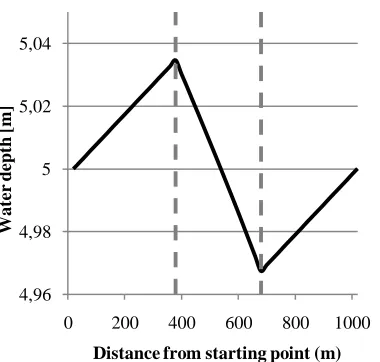
Van Urk, according to Van Velzen & Klaassen (1999) already concluded that the difference between a complete serial and parallel orientation to the flow is large. The influence of backwater effects plays a role in this serial situation. These backwater effects arise because the water can flow freely until it reaches the complete strip of rough vegetation. At this point the flow velocity decreases and the water depth will increase. This effect happens not at once and thus a backwater curve will arise before the rough vegetation where the water depth slowly increases. After the rough strip the same process takes place but there the water depth will slowly decrease again. However during the model runs that will be carried out in this study the water depth will be kept as constant as possible, just like Van Velzen & Klaassen (1999) did. This will probably eliminate the backwater effects.
One model run is carried out in order to investigate how the water depth behaves over the area. One stripe of rough vegetation is implemented, with a covering of 30 percent of rough vegetation and a water depth of 5 m. The resulting water depths in flow direction are shown in figure 15 with the black line indicating the water depth over the area and the grey dotted lines the start and ending point of the rough vegetation. That the water depth is given as input at the beginning and end of the area is very clear in this figure, both are exactly 5 m. The variation in water depth when the water flows over the area is very small, the extremes differ 0.033 m. It can be concluded that the backwater effects are very small when the water depths are kept as constant as possible and this results in a situation where the flow velocities on the area are constant.
The serial impact in this study is thus that the total area is influenced by the strip of rough vegetation and this reduces the flow velocities, and thus also the discharge and aggregate roughness, remarkable.
0 300 600 900 1200 1500 1800
50 250 450
A
d
ap
tat
io
n
l
en
gt
h
[
m
]
Width patch [m]
22
Figure 15: The water depths in flow direction, the grey dotted lines indicate the starting and end
point of the rough vegetation.
4,96 4,98 5 5,02 5,04
0 200 400 600 800 1000
Wat
er
d
ep
th
[
m
]
23
4
WAQUA COMPUTATIONS
To be able to determine what parameters have an influence on the aggregate roughness on an area, different types of situations are used in the modeling calculations. In this chapter the model runs and their results are discussed. First, in paragraph 4.1, the manner in which the aggregate Chézy value can be calculated out of the model results is given. After that the input of the model WAQUA is discussed. Here also the parameters are defined of which it is expected to have an influence on the aggregate roughness. In paragraph 4.3 the model results are given, which are the aggregate Chézy values. These results can help in finding the influence of particular parameters on the aggregate roughness and will improve the understanding of the processes that take place.
4.1
DETERMINING AGGREGATE CHEZY VALUE
To calculate the aggregate Chézy value out of the results of the model runs, the total discharge is needed. At the end of the area the total q [m2/s] is taken for all grid cells in that row. Multiplying this q
by the size of the grid cells and adding them gives the total Q [m3/s]. Because the water depth is kept
as constant as possible, the aggregate Chézy value can easily be determined using the inverse Chézy formula:
[4.1]
With:
Qwaqua = Discharge [m3/s]
h = Average water depth [m]
Wt = Width total area [m]
∆ h = Difference in water level due to the bed slope [m]
Lt = Length area total area [m]
4.2
SET UP
The input for the model can be divided in two types, fixed and variable. The fixed model input is the input that is kept constant for all situations, for example the slope. The variable input exists out of the parameters that are varied in order to investigate the influence of these parameters on the aggregate roughness. An example of the variable input is the layout of the vegetation pattern. This paragraph will describe this input, starting with the fixed input.
4.2.1 FIXED INPU T D E SCRIPT IO N
The area of investigation will have a squared shape and a slope in the bottom of 1 10-4 which is fixed
24
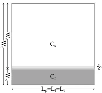
slope the water depth will be fixed at the same constant value at the beginning and end of the area during the run, the water depth above the rest of the area can vary. A cross section can be found in figure 16.
Figure 16: Cross section of the area
The size of the total area will be 1000 by 1000 m because this size was also used in the calculations done by Van Velzen & Klaassen (1999), and thus on which the WA-method is based. During the investigation two different types of vegetation are used to create the patterns of roughness types; grass and bushes. As input in WAQUA the Nikuradse k-values are given which is 0.25 m for grass and 33 m for bushes (Van Velzen & Klaassen, 1999). The Chézy value belonging to a certain Nikuradse k-value is in WAQUA calculated using the following formula (Van Rijn, 1990 according to Ministry of Transport, Public Works and Water Management (2008)):
[4.2]
With:
C = Chézy coefficient [m1/2/s]
h = Total water depth at the velocity point [m]
kn = k-Nikuradse value [m]
Max = The ‘maximum function’
The maximum function is implemented to make sure that when the 12h/kn is smaller than 1, which
happens with really small water depths and high k-Nikuradse values, the Chézy value will not become negative.
Another parameter that must be given is the eddy viscosity coefficient. This coefficient is important for the mixing width between a smooth and rough bottom, as discussed in chapter 3. The default value given in Ministry of Transport, Public Works and Water Management (2009a) is 10 m2/s and in
RWS-Waterdienst & Deltares (2009) a value of 1 m2/s is used. But in Boderie et al. (2005) and
Uittenbogaard et al. (2005) it is mentioned that an eddy viscosity of 0.5 m2/s will give the best results
and this value is normally used in model calculations, therefore it is decided to implement this value instead of the default value.
4.2.2 PARAME TER S O F INVE STI G A TIO N
In this sub paragraph the parameters are discussed that will be varied in the investigation. This is done in order to investigate whether these parameters have an influence on the aggregate roughness of the area. These parameters are defined based on factors that vary between different floodplains and on the increasing accuracy of input information that is available of floodplains. It will be explained why the parameters are taken into account and also to what extent these will be varied.
Fixed h
Fixed h ibLt
25
4.2.2.1 WA T E R D E P T H
Different water depths can occur on a floodplain, and thus when a floodplain is modeled water flows with different water depths have to be represented by the model. The prediction of the aggregate roughness, when a vegetation pattern is present in one grid cell, should be equally accurate in all times. Therefore the influence on the aggregate roughness of the water depth should be taken into account during the analysis.
Vegetation in the water will have a larger effect when the water depth is small than when the water depth is large. With the use formula 4.2 given in paragraph 4.2.1 figure 17 is made. This figure shows the Chézy values belonging per water depth for bushes (dotted line) and grass (solid line), which will be used to create the vegetation patterns.
Figure 17: Chézy value for grass and bushes for varying water depths
This figure shows that how deeper the water is, the less rough the vegetation becomes. This is because relatively a smaller part of the water column is affected by the roughness on the bottom. It is also apparent that the Chézy value for bushes becomes really small with low water depths, almost approaching to zero, and is not changing until about 3 m water depth. Therefore taking water depths smaller than 3 m is not realistic and will not give extra insight in the processes taking place.
It can be concluded that different water depths will result in different Chézy roughness values on the area, therefore different water depths will be taken into account in order to investigate what the influence is on the aggregate roughness. Furthermore it is important to investigate whether it might be necessary to include the water depth in the prediction method of the aggregate roughness. Depths of 3, 5 and 7 m are taken because it is thought that these are realistic values.
4.2.2.2 GR ID S IZ E
New developments in airborne laser scanning may lead to more precise input information to represent the floodplain and might lead to the incorporation of a finer grid. A finer grid results in a more fine representation of a vegetation pattern, and thus also the flow adjustments (see chapter 3). Because in each grid cell the basic physical properties are calculated (see chapter 2) more information on the total area will be available when smaller grid sizes are implemented. It is thus desirable to investigate whether the grid size will have an influence on the flow processes and thus the aggregate roughness on the area.
0 10 20 30 40 50
0 2 4 6 8
C
h
ez
y
v
al
u
e
[m
1
/2/s
]
Water depth [m]
26
The developments in airborne laser scanning will lead to more precise information and thus a smaller grid size than 20 m, which was also used in the experiments of Van Velzen & Klaassen (1999), will be used next to this size. Only the influence of the grid size must be investigated, all the other parameters must be kept constant, for example the sizes of the rough vegetation patches. This is a restriction in the choice of the smaller grid size, for example a grid size of 15 m is not possible because not the exact same vegetation patterns can be created as with a size of 20 m. Therefore it is chosen to use the largest value that complies with this restriction which is a grid size of 10 m, this is a factor four finer. This increase in fineness is thought to be a good representation of the influence of the grid size on the aggregate roughness. Moreover, because in every grid cell the basic physical properties are calculated, this grid size will give the least increase in calculation time.
4.2.2.3 PA T T E R N A N D C O V E R I N G
Vegetation on a floodplain is almost never uniform but very heterogeneous. Different kinds of patterns can be made based on the flow adaptation processes that evolve. The mixing layer and the adaptation of the flow play a role, but a vegetation pattern can be situated such that the adaptation of the flow does not take place in the area of investigation. A special case is the complete serial pattern, where it is not possible for the flow to redirect around the rougher patches.
PA R A L L E L OR IE N T