Normalized Weighted Averages for Tracing Continuous Trends of Data and Easy Filtering of Discontinuous Samples

Normalized Weighted Averages for Tracing

Continuous Trends of Data and Easy

Filtering of Discontinuous Samples

R. PURUSHOTHAMAN NAIR

Mission Synthesis and Simulation Group,

Vikram Sarabhai Space Centre,Thiruvananthapuram-695 022, India.

Abstract: In this paper a set of normalized weighted averages which may be called as bi-average, tri-average, quadric-average or in general kth poly average, k=2,3,4,… is introduced. The weights can be easily assigned using the integer k. The linear combination of the weights with the samples is biased to latest samples of a given discrete data set when the samples are considered chronologically or sequentially. Hence these averages can generate moving and realistic trends of data without being a moving average. Computations of these averages are not explicitly depending on the size of the data set and can be done in a progressive way. The advantage is that it is not necessary to store the data samples or its size for computing these averages. An inferring mechanism is derived based on which one can easily decide whether current sample is continuous or not with previous samples based on the computed average. Illustrative examples are presented to establish the effectiveness of this inferring mechanism in testing continuous trends and filtering of discontinuous samples of flight telemetry data of a typical launch vehicle and that of sample data sets of standard continuous signals. Mathematical properties of these averages are discussed.

Keywords: weighted averages, moving averages, wild point elimination, vector dot products, Canter’s intersection theorem, continuous trends.

1. Introduction

Weighted averages are used to prioritise data samples so that the averages can represent prominent tendencies of data sets. Many moving averages are designed to derive the trends with respect to time. These are used wherever large-scale data management is involved. There is a probability of discontinuous samples in data sets.

For example, Gardenier[1], discusses the many problems in fixing environmental standards based on moving averages and points to the probability of detecting a violation. The reason is that most environmental data are averages of successive measurements. In handling of large amount of air pollution data, Gutman [2] is cautious against using daily maximum values. Instead, application of statistical data is preferred since the maximum may be misleading. See Jackson [3], that classical method for dealing with non-uniqueness in geophysical inversion problems is to construct linear averages of the unknown function whose values are uniquely defined by empirical data. However, the usefulness of such linear averages for making geophysical inferences depends on the good behaviour of the unknown function in the region in which it is averaged. This is also fingering to the probability that the constructed linear averages may not be optimally fitting to the unknown function

Fox [4] describes several methods for converting the existing seasonal quantities into a continuous time series of fields such as dynamic height, thermocline depth, and depth-averaged density. These fields are derived using in situ data that have been acquired over many decades, but are so irregularly distributed that in most regions only annual or seasonal mean fields, an amplitude error and bias present in the seasonal values have been derived. The averages presented here will be inheriting the continuous trends of the unknown function in a better way out of such seasonal measurements and discontinuous samples can be easily filtered out.

care. Why because, in [5], it is noted that with increased utilization of health care services, positive impact on health status may not be reflected by indicators because more conditions are detected.

Trend analysis in sales and marketing area is a major filed where moving averages are contributing in a realistic way for decision-making. According to Papaioannou [6], the core component of data analysis for scientific management is statistical analysis. By emphasizing this, [6] illustrates methods of collecting, summarizing and presenting managerial data. Robb, et al. [7] compares the effectiveness of combining moving averages relative to other methods, such as simple moving averages and exponentially weighted moving averages, where particular attention is placed on methods for selecting the number of periods employed, and on handling noisy data. Thus it undermines the role of making the data smooth by filtering out noisy samples.

Here certain weighted averages are proposed using normalized weights. These normalized weights can be defined using positive integers, k=2,3,4,…,N. When k=2,

the average may be called bi-average, k=3, it may be called tri-average and when k=4, the average may be called quadric-average. In general it may be called kth poly average. These averages are biased more and more to the latest data samples when the samples are considered either sequentially or chronologically. As a result, these averages can bring out the moving data trends in a realistic way without being a moving average. Computations of these poly averages are not explicitly depending on the size of the data set and they can be computed in a progressive way. Hence one need not be concerned with storing the data or its size for the purpose of computing these averages.

The influence of a leading sample over kthpoly average will go on getting reduced at the rate of 1/kn-1

for a set of size n and as n grows. The contribution of the latest sample to the average is always maintained as

(k-1)/k, independent of the sample size n. It is proved using Canter’s intersection theorem that series of computed averages preserve the trends between the consecutive samples considered as the process progresses. When considered as a dot product, generating these averages is a continuous process belonging to the conjugate space of the Euclidian vector space R2.These averages also can be considered as continuous linear functions in real Hilbert spaces Rn , n=2,3,… An isometric isomorphism associates the vectors of R2 to the averaging process.

These poly averages are sensitive to the order in which the samples are considered. It can be proved that contribution of a leading sample to the average can be reduced in a fast way using these averages. They converge to the arithmetic mean when data samples are too close to each other and perturbations are keeping a diminishing trend as the sample size grows.

The set of kth poly averages computed sequentially on a set of discrete samples of a continuous and monotonically increasing signal will also be monotonically increasing. The poly average data curve follows the actual data curve more closely than the moving average using common mean. This way data trends are more inherited to these poly averages from the parent data compared to a moving average using the common mean as far as continuous data samples are concerned.

The averaging process can be best treated as a vector space dot product operation and are continuous linear functions in real Hilbert Spaces Rn, n=2,3,… and is analysed in that way. Theoretical properties of these averages are presented.

2. Poly Averages and their Properties

Definition 2.1

Given {x1 , x2 , x3 ,…, xn } , a set of n real numbers, k th

poly average of a single entry x1is defined as

a1 = (x1 +(k-1)x1)/k (2.1)

Thus kthpoly average of a single entry is the entry itself, same as the case with common mean. The kthpoly average of entries x1 , x2 , x3 ,…, xi ; i  2 , is defined as

From (2.2), it follows that in general an the kthpoly average of x1, x2, x3 , x4 ,… xn is computed out of

an-1,the k th

poly average of x1 , x2 , x3 , x4 …. and xn-1 using the equation

an = (an-1 +(k-1)xn)/k (2.3)

Proposition 2.1

The computation of the kth poly average ai of x1, x2, x3 , x4 ,…and xi out of ai-1 is not depending on i,

the number of samples considered, for i=1,2,..,n.

Proof: From equations (2.3) it follows that for computing ai, it only requires ai-1 , the previous average and the current sample xi. Also more significantly, one need not depend on i, the number of samples considered.

Note 2.1

In equation (2.2), all samples are explicitly considered and the role of i is also explicitly presented. While (2.3) is the computational procedure, (2.2) is an analytical equation clearly indicating that ai is depending on all the previous data samples and is not a moving average in that sense.

Note 2.2

The bi-average, tri-average and quadric-averages may be derived form (2.2) as follows:

Example 2.1

The bi-average of x1, x2, x3 , x4 ,…and xn isobtained as

an = x1 / 2n-1 + x2 / 2n-1 + x3 / 2n-2+… +xn / 2 (2.4)

Example 2.2

The tri-average of x1, x2, x3 , x4 ,…and xnisobtained as

an = x1 / 3 n-1

+ 2x2 / 3 n-1

+ 2x3 / 3 n-2

+… +2xn / 3 (2.5)

Example 2.3

The quadric-average of x1, x2, x3 , x4 ,…and xnisobtained as

an = x1 / 4n-1 + 3x2 / 4n-1 + 3x3 / 4n-2 +… +3xn / 4 (2.6)

Proposition 2.2

The kth poly average an of x1, x2, x3 , x4 ,…and xn is least biased to x1 , its biases are strict

monotonically increasing and that the average is most biased to the last sample xn.

Proof: From (2.2), it is clear that the weight coefficients 1/kn-1, (k-1)/kn-1, (k-1)/kn-2, …, and (k-1) / k of x1, x2, x3

,…and xn respectively are strictly increasing. Hence in an, the majority of its content is (k-1)/k of xn and it is formed least out of the first sample, with only 1/kn-1 of x1. Thus the kth poly average is biased more and more to the latest samples.

The situation with respect to the common mean can be compared in respect of weight distribution. In common mean since the weights are uniformly assigned to all the samples, the current sample has only a weight

1/n and cumulative weights of all previous samples put together is (n-1)/n. This is in a way just the opposite of the situation with respect to poly averages. In poly averages, (k-1)/k is the weight to the current sample and 1/k is the cumulative weight to previous samples.

Proposition 2.3

The kth _{poly averages a}

1 , a2 , a3 , …, an of x1, x2, x3 , x4 ,…,xn will be of increasing order when x1,

x2, x3 , x4 ,…,xn are of increasing order.

Proof: This is an immediate consequence of proposition 2.2 Proposition 2.4

The weights 1/kn-1, (k-1) / kn-1, (k-1) / kn-2, …, and (k-1)/k are normalized.

Proof: In(2.3) only two weight coefficients are considered. These are 1/k and (k-1)/k and clearly these are normalized. In (2.2), the weight of xnis retained as (k-1)/k. Thus as and when a new sample is added, the maximum weight is assigned to it. As far as the remaining weights are considered, these are reduced at a rate

1/k. From (2.3), it follows that the remaining n-1 weights always satisfy the equation,

1/k

)/k

1

(k

1/k

(n-i)

2 -n 1 i -1

n











(2.7)

This way the weights are normalized.

Proposition 2.5

The set of weights {1/kn-1, (k-1)/kn-1, (k-1)/kn-2, …, (k-1) / k } generates a convex set of averages.

Proof: By proposition 2.4, the weights are normalized. Also equation (2.3) is a standard convex linear combination of the general form

x

φ



x(1



φ

);

0



φ



1

. Hence the set

{

a

₁

,

a

₂

,

a

₃

,...,

a

_n-1

,

x

_n

}

is a convex set.

Proposition 2.6

The kth poly averages a1 , a2 , a3 , …, an of x1, x2, x3 , x4 ,…,xn will be sensitive to the order in which

the samples x1, x2, x3 , x4 ,…,xn are considered.

Proof: Since a1 , a2 , a3 , …,an are biased to the last samples, they change with the order in which the samples

x1, x2, x3 , x4 ,…,xn are considered. For example, when the samples are arranged in ascending order and the averages are computed, then the averages also will be in ascending order by proposition 2.3. Similarly the averages will be of descending order if the samples are so, because of the convexity of the set

}

{

a

₁

,

a

₂

,

a

₃

,...,

a

_n-1

,

x

_n . Thus the trends of the data are inherited to the averages.

Note 2.3

When

x

i



x

i-1



x

i-1



x

i2

;

i



3,4,...,

n

-

1

:

x

i



0

;

i



1,2,...,

n

, bi-averages will satisfy the

equation

n

2,3,...,

i

)/2;

x

(x

a

_i



_i



_i-1



(2.8)

This is also because of the convexity in (2.3).

Note 2.4

As the weight of the latest sample xn is always maintained as (k-1)/k, from (2.3), it is clear that when the samples x1, x2, x3 , x4 ,…,xn are non-negative and of increasing order, all poly averages will satisfy the equation

n

1,2,...,

i

;

1)/k)x

-((k

a

x

_i



_i



_i



(2.9)

fixed. It can be proved that poly averages are a continuous mapping when

x

i



x

i-1



x

i-1



x

i2

;

i



3,4,...,

n

.

The following proposition shows that trends from sample to sample is maintained by the averages and will closely follow the continuity of data.

Proposition 2.7

When

x

i



x

i-1



x

i-1



x

i2

;

i



3,4,...,

n

, the poly averages will satisfy the inequality,

n

,4...,

i

;

a

-a

a

a

_i



_i-1



_{i-1 i-2}



3

(2.10)

Proof: When the samples x1, x2, x3 , x4 ,…,xn are non-negative and of increasing order, the averages satisfy the inequality,

x

i



a

i



x

i-1

;

i



2,3,...,

n

and they too are of increasing order. Further by (2.9), the series of

computed averages satisfy the inequalities

n

2,3,...,

i

);

x

-1)/k)(x

-((k

a

a

i



i-1



i i-1



(2.11)

n

3,4,...,

i

);

x

-1)/k)(x

-((k

a

a

_i-1



_i-2



_{i-1 i-2}



(2.12)

From (2.11) and (2.12), it follows that (2.10) is true.

The mapping of xi to ai is actually a continuous function as below.

Proposition 2.8

Let the samples x1, x2, x3 , x4 ,…,xn are non-negative and of increasing order. Let

ε



0

be given such that

x

_i

-

x

_i-1



ε

. Then it can be obtained a corresponding

δ

such that

0



δ



ε

such that

a

_i

-

a

_i-1



δ

.

Proof: When the samples x1, x2, x3, x4,…,xn are non-negative and of increasing order, the averages satisfy the inequality

x

_i-1



a

_i



x

_i

;

i



2,3...,

n

(2.13)

As a consequence of (2.11) and (2.13) we have,

ε

x

-x

a

a

)

x

-1)/k)(x

-((k

i i-1



i



i-1



i i-1



(2.14)

Form (2.14), if we choose

δ



x

_i



x

_i-1 then

δ

a

a

ε

;

δ

0

ε

x

x

_i



_i-1









_i



_i1



(2.15)

Equation (2.15) proves the required result. If we recall from Walter Rudin [8], (2.15) is the definition of continuity at a given point xi. Later we will prove that

(a

i



a

i-1

)



δ



(x

i



x

i-1

)

as the process

advances.

So when

x

_i-1



x

_i and comes arbitrarily close to xi, the average ai-1 also tends to ai andapproaches it in a corresponding way.

Note 2.5

Proposition 2.9

The kth poly averages of x1, x2, x3 , x4 ,…,xn will be converging to the arithmetic mean when x1, x2,

x3 , x4 ,…,xn are sufficiently close to each other.

Proof: This is an immediate consequence of the fact that the normalized weighted sum of x will be x itself. Hence when the samples are tending to some constant, the averages also will converge to the same constant in accordance with proposition 2.8.

3. Poly Averages as Dot Product of Vectors.

Consider the vector y=[1/k (k-1)/k]T. Then equations (2.3) can be expressed as dot product of y and vector yn=[an-1 xn]T as

f(yn)=y T

yn = an (3.1)

If we recall from [9], that any arbitrary continuous linear function f of the conjugate space X* of a Hilbert space X is of the form

f(x)=(x, y) (3.2)

where (x, y)= yTx is the dot product of x and y ,

x,

y



X

; y is a fixed unique vector specific to the given continuous linear function or simply functional f.

Thus the ploy averages presented here are nothing but scalar valued continuous linear functions defined over the real Euclidian vector space R2 whose range is the real line R1. Since the vector

T

1)/k

-(k

1/k

y



[

]

is such that the closed interval

[

1/k,

(k



1)/k

]



[

0

,

1

]

, the averaging function f is a convex function and the set of averages {a1 , a2,…, an} is a convex set.

Equations (3.1) to (3.4) linking the average to a fixed vector y=[1/k (k-1)/k]T is a rich mathematical property of this average as a member of the conjugate space of R2. The mapping

y



f

is an isometric isomorphism.

Theorem 3.1

If d is the metric defined in R2 then

d(a

n

,

a

n-1

)



d(x

n

,

x

n-1

)

as

n





and when

)

x

d(x

)

x

d(x

;

x

x

_i-1



_{i i}

,

_i-1



_i-1

,

_i-2 ; i=1,2,3,…n,,…



.

Proof: Let









d(x

x

)

d(x

x

)

i

1,2,...n..

.

p

i-1

,

i i-1

,

i-2

;

(3.3)

Consider the closed intervals,







p

(a

-

a

),

p

i

1,2,...,

n,...

C

i

[

-

i i-1

];

(3.4)

Then by propositions 2.6 and 2.7 the closed intervals in (3.4) satisfy the conditions,

0

)

d(C

,

n

1,2,....;

n

C

C

_n-1



_n

,







_n



(3.5)

Let C be the intersection of these closed sets.



 



1 i i

C

C

(3.6)

 

p

C



(3.7)

The result (3.7) shows that the averages closely follow the steady trend of the sample space and catch up with this trend as n advances.

4. Inferences from Poly Averages.

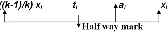
When a huge amount of discrete data samples of a continuous signal are available, how to trace the continuity of the data set is what we have discussed in the preceding sections. In this situation, according to result (2.15), it is clear that continuity is a local issue relevant to current sample. So an averaging mechanism, which moves along the data, will be more suitable. From (2.15), it is also implied that, it should reflect the past trend in such a way that more a data sample is near to current sample, it should be of more weight. Also one should be able to infer the status of the current sample based on the current average. Equations (2.3), (2.9) and (3.7) are to be understood in this back ground. When

a

_i



((k



1)/k)x

_iit is clear from (2.3), that xiis getting isolated from the previous samples and previous samples are having insignificant contribution compared to the current one (ref. fig. 4.1 below). It is the beginning of a new trend or it can be a discontinuous sample. By conducting the test derived from (2.9) as illustrated in fig. 4.1 below, with a sufficient number of samples, say,

xi+1, xi+2, xi+3, … xi+m, it can be confirmed whether xi is indeed an isolated wild sample or not. Suppose all these m samples are not following the trend obtained for xi. Then xi can be taken as an isolated discontinuity. On the contrary, if the tests are showing that all the m samples are following similar trend as xi, then it is a new trend. The averaging mechanism can be reset. When

a

_i



x

_i, it is a steady state and if simultaneously (3.7) also is true, the system is passing through a healthy phase and the averaging mechanism can continue the state. This is what figure 4.1 illustrates.

Fig. 4.1 Ideal averaging status

(Refer the attached flow-chart as annexure-1 for implementing this test derived from the inequality 2.9)

From the inequality (2.9) and equation (2.3), it is clear that

a

_i



x

_iwhen

a

_i

/k







x

_i

/2k



. That is the past samples are contributing to the average in a considerable way so that the situation in figure 4.1 is true. If









x

/2k

/k

a

i i , then it can be inferred that current sample xi is predominating over past samples. It can be the beginning of a new trend or a wild or discontinuous sample. Thus the half way criterion in figure 4.1 can be set as below.

i i

i

(k

1)/k)x

(1/2k)x

t







(4.1)

So if

a

_i



t

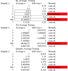
_i, then xi is a discontinuous sample.

Here there is an asymptotic characteristic exists with weight distribution at each stage of averaging after computing, say m averages where this m can be fixed depending on the poly average index k. For example

Example 4.1

This situation is numerically illustrated in table 4.1 as below for bi-average, tri-average and quadric average.

Bi_Average Testing

Sample-x Average-a half-way-t Remark

1 1 0.75 cont-ok

2 1.5 1.5 cont-ok

3 2.25 2.25 cont-ok

5 3.625 3.75 discontinuity

6 4.8125 4.5 cont-ok

100 52.40625 75 discontinuity

7 5.3125 5.25 cont-ok

Tri-Average Testing

Sample-x Average-a half-way-t Remark

1 1 0.833333 cont-ok

2 1.666667 1.666667 cont-ok

3 2.555556 2.5 cont-ok

5 4.185185 4.166667 cont-ok

6 5.395062 5 cont-ok

100 68.06173 83.33333 Discontinuity

7 6.061728 5.833333 cont-ok

Quadric-Average Testing

Sample-x Average-a half-way-t Remark

1 1 0.875 cont-ok

2 1.75 1.75 cont-ok

3 2.6875 2.625 cont-ok

5 4.421875 4.375 cont-ok

6 5.605469 5.25 cont-ok

100 76.40137 87.5 Discontinuity

7 6.651367 6.125 cont-ok

Table 4.1 Comparison of Poly Averages for detecting wild samples

The example in Table 4.1 is considered as a typical illustrating data set in order to demonstrate how the averages are performing when the samples are uniformly increasing and the application of inequality (2.9) in detecting discontinuous sample. When the index k is increasing, note that the averages are more closely following the data as the bias are more and more lenient towards the current sample.

From Table 4.1, it is clear that bi-average is more sensitive to discontinuity and other averages are more accommodating as illustrated by the presence of sample data 5 in coloumn-1. When a comparatively large sample 100 is introduced in column-1, all averages are responding to it in uniform way to pinpoint it as a wild entry. Also note that, how the averages are responding to the very next normal sample following a wild sample. Thus normalcy of continuity is easily traced by all the averages.

Significantly consider the benefits as listed below. i. Poly averages are based on all the previous samples.

ii. They are more close to the data samples than common moving mean.

iii. They are more sensitive to the current trends in data and influence of earlier samples becomes insignificant as the process progresses. For example, the presence of a wild sample at any stage is better handled by these averages. For example, if the very first sample is a discontinuous sample, it can also be caught by a reverse order of averaging.

iv. When one wants to get an idea of the parameter ranges, they are more realistic. v. Simplicity in computing the averages.

vii. Poly averages are having a moving tendency by virtue of the weight distribution even though they are computed out of all the previous samples.

Wu et al. [11], presents the global atmospheric circulations statistics using four year averages of the monthly mean global structure of the general circulation of the atmosphere in the form of latitude-altitude, time-altitude, and time-latitude cross sections. Similarly consider the case with the solar energy report [12] on long-term monthly averages of solar radiation, temperature, degree-days and global K(sub T) for 248 National Weather Service stations and direct normal solar radiation. This type of tabular representation of atmospherics data can be better handled by these poly averages because of the particular weight distribution and their convenient decision making feature (4.1) with respect to discontinuous samples or violations.

5. Data Retrieving from Poly Averages.

Compared to other weighted averages, data may be easily retrieved back if the averages are known. Consider this process of retracing the data from the computed averages.

an = x1/k

n-1

+((k-1)x2)/k n-1

+((k-1)x3)/k (n-2)

+…+((k-1)xn)/k (5.1)

an-1 = x1/k (n-2)

+((k-1)x2)/k (n-2)

+((k-1)x3)/k (n-3)

+…+((k-1)xn-1)/k (5.2)

xn =( k*an- an-1)/(k-1); n>1. (5.3)

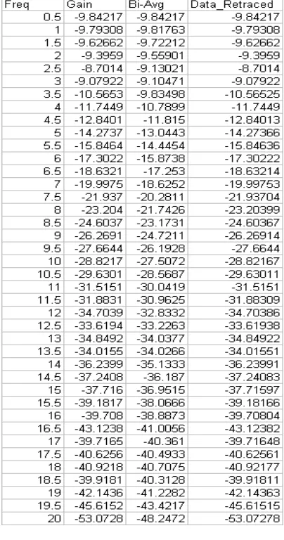
Example 5.1

By repeatedly applying equation (5.3), data can be recreated. As an illustrative example, consider gain characteristics of a typical actuator listed in table 5.1. The bi-averages are computed and then gain data are retrieved using (5.3) in column-4.

Table 5.1 Gain Data retraced from bi-averages

the data is increasing, decreasing or steady. Here also, these poly averages will be more effective as they are better candidates representing the past trends along with the status of the current sample. Also note that data samples can be easily recreated from consecutive averages.

6. Application of Poly Averages in Tracing Continuity of Data.

As an application of these averages, these are implemented in a graphic package in order to follow the continuity of data, eliminate wild points and generate appropriate minimum and maximum bounds.

Example 6.1

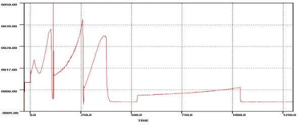
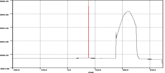
As a test case, a typical satellite launch vehicle data is considered. Fig.6.1 is the plot while taking into account the wild samples also. After processing through bi-average, the plot is as in Fig-6.2 and the averaging process reported the following information. It has to be reported here that no sample is rejected from plotting and only parameter bounds are derived from the data by discarding those wild samples. Then the parameter data is plotted with these new bounds. Also in the detailed reporting by the application, many discontinues samples are identified.

Averaging Range Min : -01.333725 Averaging Range Max : 41.935726

Averaging Range Min Time: 263.000000 Averaging Range Max Time: 259.500000

Actual Range Min : -01.333725 Actual Range Max : 6583916953600.000000

Actual Range min Time: 263.000000 Actual Range Max Time : 113.500000

Fig. 6.1 Parameter Plot Affected by Wild Samples around x=113.00 seconds.

Fig. 6.3 Parameter plot with wild samples accounted for deriving bounds

Example 6.2

Consider Fig 6.3 above. The parameter data in this plot is another test case. Here discontinuous entries can be seen in the plot. This parameter, when processed through bi-average, the discontinuities are ignored and appropriate bounds are fixed as in Fig.6.4

With respect to this parameter data the averaging process extracted the following information.

Averaging Range Min : -00.463844 Averaging Range Max : 05.285851

Averaging Range Min Time: 515.156616 Averaging Range Max Time: 331.139720

Actual Range Min : -00.463844 Actual Range Max : 12.113614

Actual Range min Time: 515.713672 Actual Range Max Time : 114.354824

Significantly, the minimum value is reported as -00.463844 at time 515.156616 seconds flight time. The data ends at 521.24327. Consider the actual minimum reported. During this period, all samples are not of this value and there is discontinuity with further dip. Thus the reporting is keeping a track of continuity in a close way so that even a small pulse will be discarded if it is not with in the currently judged bounds.

Fig 6.4 Parameter data plotted with modified bounds-discarding wild samples using bi-average

Example 6.3

Fig. 6.5 A Parameter plot pointing to the appropriateness in fixing bounds by the process.

What being lime lighted is that even if there are no wild points presented in the data, the averaging process is useful to bring out appropriate bounds for the parameter data and data can be smoothened by using the averages instead of discontinues data samples.

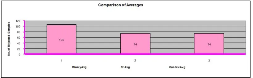
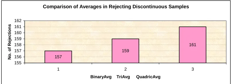
The chart below in figure 6.6 provides a comparison of rejection of data samples by the binomial, trinomial and quadric averages for a typical analog flight parameter. It is clear from the chart that as established in Table 4.1, that binary average is stricter with discontinuous samples than other averages.

Fig 6.6 Comparison of rejection of discontinuous data samples by the Poly Averages on a typical flight parameter data.

The total entries in this case are 401,464 and among this large set of data, the averaging process discards only very negligible amount of discontinuous samples. Thus the averages really are effective in identifying the continuity of data for a real life situation.

Example 6.4: Tracing continuous trends of standard data signals.

Fig 6.7 Sin(x) data samples –Manipulated with wild entries

Fig 6.8 Sin(x) data samples –After Discarding wild entries

Note that the natural bounds of the signal were traced by the bi-average in this case.

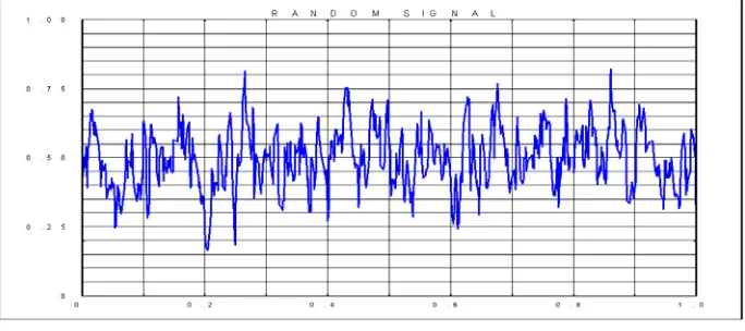
Fig 6.10 Random signal after discarding wild entries using Bi-Average

Here random signal is neither continuous nor it is uniformly increasing. But when processed through the bi-average, the appropriate data bounds are traced and the signals are displayed in the correct perspective. Thus it undermines the usefulness of the process in determining the natural signals from the given domain that may be corrupted with disturbances. It may be referred here the work by Tokumaru and sakai [14], discussing trends in random data analysis.

Another test is conducted on random signals in open interval (0 1) using the bi-average. The bi-average process is repeated on previous set of averages so as to obtain a set of third level bi-averages. These are presented in the Fig 6.11 below. The random characteristics of the data will be reduced if further levels of averages are obtained and it will be converging to the uniform distribution y=0.5 in this case.

Fig 6.11 3rd Level Bi-Averages of Random Signal

It is very clear that with the random test signals, the bi-average process will converge fast to this uniform distribution than tri-average or quadric average or other poly averages. The reason is that among the poly averages, it is more sensitive to the random or discontinuous trends presented in the data as illustrated in Table 4.1 of section-4 using the test criterion based on Fig. 4.1 of Scetion-4. Compared to other poly averages, only 50% of the current data sample is contributing to the bi-average, which is less than that of other poly averages. Thus the random characteristic of the data is more excluded in bi-average compared to other poly averages.

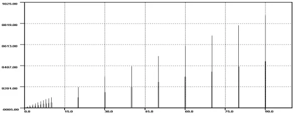
Fig 6.12 Data Sample Plot of Binomial distribution with wild entries

(No. of trials is 10 and 1 success in 10 trials)

Fig 6.13 Data Sample plot of Binomial distribution redeemed using bi-average

(No. of trials is 10 and 1 success in 10 trials)

Martz and Kvam [16], presents a graphical method in determining statistically significant trend or pattern over time in an underlying Poisson event rate of occurrence or binomial failure on demand probability using exponentially weighted moving averages. This test points to a similar result by retrieving original trend.

These experiments validate that indeed the averages are capable to trace the continuous trends of standard test signals and to derive the natural ranges in which these signals operate.

Comparison of Averages in Rejecting Discontinuous Samples

157

159

161

155 156 157 158 159 160 161 162

1 2 3

BinaryAvg TriAvg QuadricAvg

No. of Rejections

Chart 6.15 is a typical rejection pattern of the averages with random signal data samples. The averages are almost evenly rejecting the discontinuous trends of the random data set.

7. Conclusions

The poly averages presented here are based on the theoretical definition of continuity of data and at the same time, they are providing a very simple solution to the vital problem in many areas of day to day life - whether current value of a variable is continuous with the past trend or it violates this trend. For example, in environmental parameter fixing, health and health care, customer and market trend analysis etc. these averages can contribute in a successful way and bi-average will be stricter with respect to discontinuous data samples.

The averages presented here are found to be tracing the trends of the data as the sample set is growing with time, even though they are not moving averages. The normalized and convex weights of the averages provide an inbuilt moving tendency to them and associate these averages with classical mathematical properties. There is accountability, where the average will be, with respect to the current sample. Generally as continuous linear functions, the averages will be successful in tracing continuous trends of any natural or artificial process.

Acknowledgements

Author is much indebted to Dr. G. Madhavan Nair, late chairman, ISRO, for the support provided in pursuing these studies. Author wishes to express the sincere and profound gratitude to Shri TR Chidambaram, Director, IISU for the valuable directions given to this work. He is very much thankful to Dr. B. Nageswar Rao, Head, SDA, Structures, VSSC, Prof. Dr. M.R. Kaimal, dept. of Comp. Sci., Amritha University, and Editorial Committee members of VSSC, especially Director, VSSC, for clearing this paper for publication.

References

[1] Gardenier, T.K,Moving averages for environmental standards Simulation, Vol.39, Issue-2, 49-58, Aug, 1982,

[2] Gutman, A., Computer Techniques in Environmental Studies III, Proceedings of the Third International Conference on Development and Application of Computer Techniques to Environmental Studies, 255-270, 1990.

[3] Jackson, D.D., The use of a priori data to resolve non-uniqueness in linear inversion, Geophys. J. R. Astron. Soc., Vol.57, Issue-1, 137-157, April-1979,.

[4] Fox. D.N, Fitting Seasonal Averages with a Continuous Function, Shared Bibliographic Input, NORDA-246, Apr 1991

[5] Wilson, R., Feldman, J.J., Kovar, M.G., Continuing Trends in Health and Health Care, Annals of the American Academy of Political and Social Sciences, Vol-435, p140-156, Jan 1978.

[6] Papaioannou, T., Data analysis in management, Computers: Applications in Industry and Management. Proceedings of the International Seminar, 185-209, 1980.

[7] Robb, D.J., Silver., E.A., Using composite moving averages to forecast sales, Journal of the Operational Research Society, Vol. 53, Issue-11, 1281-1285, Nov. 2002,.

[8] Walter Rudin, Principles of Mathematical Analysis, McGraw-Hill Book Company, NewYork, 1953.

[9] Simmons G.F., Introduction to Topology and Modern Analysis, McGraw-Hill Book Company, NewYork, 1963.

[10] Hall, W.J., Efficiency of weighted averages, Journal of Statistical Planning and Inference, Elsevier Science B.V, Vol. 137, Issue -11, Nov. 2007,

[11] Wu, M.F, Geller, M.A., Nash, E.R., Gelman, M.E. , Global Atmospheric Circulation Statistics: Four Year Averages, NAS 1.15:100690; REPT-87B0437, Jun 1987.

[12] Solar Energy Research Inst., Golden, CO. Insolation data manual: Long-term monthly averages of solar radiation, temperature, degree-days and global K(sub T) for 248 National Weather Service stations and Direct normal solar radiation data manual: Long-term, monthly mean, daily totals for 235 National Weather Service stations. Addendum to the Insolation data manual SERI/TP-220-3880, Jul 1990.

[13] Salatian, A., Hunter,J., Deriving trends in historical and real-time continuously sampled medical data, Journal of Intelligent Information Systems, Integrating Artificial Intelligence and Database Technologies, Vol.13, Issue 1-2, 47-71,1999.

[14] Tokumaru, H., Sakai, H., Recent trends in random data analysis, JSME International Journal, Vol.30, Issue- 259, 14-21, Jan., 1987. [15] Beschta, Robert L, Moving averages and cyclic patterns(note), Journal of Hydrology New Zealand, Vol. 21, Issue-1, 148-151, 1982. [16] Martz, H.F., Kvam, P.H., Detecting trends and patterns in reliability data over time using exponentially weighted moving-averages,

Annexure-1

Algorithm for tracing continuity of data