BIASED RANDOM
ENERGY-EFFICIENT ROUTING ALGORITHM
(BREERA)
Barra Touray
Engineering, Liverpool John Moores University, Byrom Street, Liverpool, L3 3AF, United Kingdom
[email protected] http://www.ljmu.ac.uk/ENG/index.htm
Dr Princy Johnson
Engineering, Liverpool John Moores University, Byrom Street, Liverpool, L3 3AF, United Kingdom
[email protected] http://www.ljmu.ac.uk/ENG/index.htm
Abstract:
A Wireless Sensor Network (WSN) is a network of spatially distributed autonomous devices that depend on their sensors to monitor environmental or physical conditions and report to a base station. The topology of any network is important and wireless sensor networks (WSNs) are no exception. In order to effectively model an energy-efficient routing algorithm, the topology of the WSN must be factored in. There has been much research into regular topologies for WSNs, to efficiently save energy and hence extend the lifetime of the network. However, little work has been done on routing within patterned WSNs, except for the shortest path first (spf) routing algorithms. The issue with the spf algorithm is that it requires global location information from the sensor network, which proves to be a drain on the network resources. In this paper a Biased Random Energy-Efficient Routing Algorithm is proposed (BREERA). It is based on random walk and probability. It uses probability theory to acquire all the information it needs to route packets based on the energy resources in each node and thus does not require any global information from the network. It is shown in this paper that BREERA uses the same energy as the shortest path first routing in cases where the message to be sent is comparatively small in size compared with the inquiry message among the neighbors. It is also shown to balance the load (i.e. the packets to be sent) among the nodes in the network. In most of the WSN applications the messages sent to the base station are very small in size. Therefore BREERA is viable and can be used in sensor networks employed in such applications. In this research paper, BREERA has been demonstrated to be a statistically and empirically effective WSN routing algorithm.
.
Keywords: biased random walk; routing algorithm; shortest path first; wireless sensor network.
1. Introduction
WSNs are used in various applications such as environmental monitoring, danger alarm and medical analysis. The developments in low-power and small form-factor processors, equipped with wireless communication capabilities and sensors allow for the employment of large-scale, extremely dense sensor networks in such applications [1] [2]. The sensor nodes are so tiny that their energy supply, storage space, data processing and communication bandwidth are very limited and hence every possible means of conserving the usage of these resources is aggressively sought. In WSNs the energy of the nodes is especially a valuable commodity and hence various schemes such as the WSN topology, routing algorithms or MAC protocols have been used to conserve energy and hence maximize the network lifetime [3] [4][5]. In this research paper, novel techniques for both the topology and routing algorithms are proposed for this purpose.
number of nodes deployed, and the limited energy and computational power available to the nodes. As the routing protocols based on random walk do not require global information they prove to be suitable for WSNs [6]. Moreover in small-size data applications it can be proved statistically that random walk is as energy efficient as the shortest path algorithm which uses the least energy between source and destination. Random walk also achieves load balancing in a network and thus avoids partitioning of the network as the shortest path algorithms tend to do. Therefore this research paper focuses on routing algorithms for small-size data transmission in square grid patterned WSNs using BREERA.
The use of random walk in WSNs has been extensively researched [7], of which the Directional Rumor Routing in Wireless Sensor Networks is based on the random walk of agents. The aim of this algorithm is to improve the latency and energy consumption of the traditional algorithms using propagation of query and event agents in straight lines, instead of using purely random walk paths. Directed Rumour Routing has two phases for calibration. In the first phase each node sends a Hello message stating its position to each of its neighbor. The hello messages are used by the receiving nodes to record their neighbors and their positions. During the second phase each node tests whether it is at the edge of the network. When a node senses an event it creates a number of event agents and propagates them into the network along some linear paths forming a star-like propagation trajectories. These event agents are not allowed to pass the edge nodes. After this a node is randomly chosen as the sink node. The sink node creates some query agents for each fired event. Each agent contains the id of the current node, the id of the previous node (depicting the direction of events), location information of the source node, and a table containing the ids of the events and distances to them. The disadvantage with this method is that the hello messages drain the WSN of its limited bandwidth and imposes additional energy drain on the nodes. So, in BREERA the need for hello messages has been eliminated.
In [6] a routing protocol based on random walk for a square grid topology has been proposed. This routing algorithm does not require any global location information and achieves an inherent load balancing property for WSN, which is difficult to achieve with any other routing protocol. The probability of successful transmissions from the source to the destination by random walk was analyzed statistically, and it is proved that this protocol is as energy efficient as the shortest path routing algorithm with the assumption that the message to be sent is small in size compared to the inquiry message among the neighbor nodes. This random walk protocol is purely based on equal probability and hence it may not be energy efficient in selecting the next-hop. However, the BREERA proposed in this research work uses probability to enable the nodes to make a fair guess about the energy level of their neighbors and select the neighbor with the maximum energy to forward the message packet, and hence this is different from the algorithm proposed in [6].
The rest of the paper is organized as follows. In section 2 a review of the related work is presented while in section 3 the proposed BREERA algorithm is discussed. The statistical and empirical analyzes of BREERA are presented in sections 4 and 5 respectively. Section 6 concludes the paper.
2. Related Work
In recent years, WSNs have been attracting rapidly increasing research efforts [8] [9] [2]. Research into routing protocols has been the major highlight of research in WSN. The traditional routing schemes proved unsuitable to adapt to WSNs due to the specific characteristics of WSNs and many new algorithms that can support WSNs [10] [11] [5] [6][12][13] have been developed.
In [10] Energy Prediction and Ant Colony Optimization Routing (EPACOR) technique is proposed. In this routing algorithm when a node needs to deliver data to the sink, ant colony systems are used to establish the route with optimal or sub-optimal power consumption, and meanwhile, learning mechanism is embedded to predict the energy consumption of neighboring nodes when the node chooses a neighboring node to be added to the route. In this algorithm, a mechanism is used to find the route with maximum remaining energy to the sink (remaining energy of a route is defined as the minimum remaining energy of all the nodes in the route). The nodes visited by an ant are recorded to avoid loops in building up a route to the sink. However the maximum remaining energy of nodes for a particular route might include some nodes with minimal energy thus depleting the energy of those nodes resulting in the partition of the network [4].
along the least cost path between the source SN and the BS. If it is, then it rebroadcasts the message to its neighbors. This is repeated until the message gets to the BS. The process of each sensor node acquiring the knowledge of the least cost path between itself and the base station is as follows. In the initial stage, each node sets its least cost path to the base station to infinity. The BS then broadcasts a message to all the nodes in the network with the cost set to zero. A receiving node verifies whether the estimate in the message plus the link cost on which the message was received is less than the current estimate. If it is true, the current estimate and the estimate in the broadcast message are updated accordingly and the message is then re-broadcast, otherwise nothing happens. There is a potential problem here in that the nodes farther away from the BS will get more updates and some nodes may even have multiple updates. The MCFA has been modified with the back-off algorithm to solve this problem in [11].
In [12] [13] Level Biased Random Walk for Information Discovery in Wireless Sensor Networks is proposed (LBRW). In LBRW, a search packet is originated by the sink and it traverses along a random path to one of the nodes on the circumference and traverses back to the sink along a random path. These two paths will most likely be different. This is repeated until the target information is discovered. The LBRW protocol needs nodes to be aware of their corresponding neighbor level and their own level. A node level is the number of hopes it is away from the sink. For nodes to get their levels, the sink nodes broadcast a packet known as LevelInformation packet setting its level as zero. A node that received this packet updates its level equal to the level in the LevelInformation plus one. It also updates the packet by its level information and then rebroadcasts the packet. A node might receive multiple LevelInformation packets but it sets its level to the minimum value received. Nodes then divide their neighbors into LowLevelNeighbors and HighLevelNeighbors each containing neighbors that are level below the node and level above the node respectively. These tasks are executed one time at the setup of the network. This contains lots of overhead and might drain the batteries off their limited energies. In [13] two more protocols Several Short Random Walks (SSRW) and Random Walk with Level Biased Jumps (RWLBJ) were proposed which use a combination of random and level biased steps to search for the information similar to LBRW.
In [6] the Random Walk Routing for Wireless Sensor Networks, a routing protocol based on random walk for a square grid based network topology is proposed. The proposed routing algorithm does not require any global location information and achieves load balancing for the WSN. The probability of successful transmissions from the source to the destination by random walk was analyzed statistically and proved to be as energy efficient as the shortest path routing algorithm with the assumption that the message to be sent is small in size compared to the inquiry message among the neighbor nodes.
The algorithm provides load balancing in the WSN but the nodes near the base station are inevitably under heavier load than the nodes further from the base station. To remedy this situation a density-aware deployment scheme was used to guarantee that the heavily-loaded nodes do not affect the network lifetime even when exhausted.
In traditional random walk algorithm, all the nodes have equal probability of being selected. Hence, this results in poor energy-efficiency of the sensor network. Whereas, BREERA which is a modified version of the traditional random walk protocol, selects the next-hop node based on the remaining energy levels of the nodes. Therefore, this scheme offers much better energy-efficient routing methodology.
Sensing and connectivity are vital parameters in a WSN. For energy efficiency it is important to use a minimum number of sensors possible while maintaining the connectivity to cover a sensing area in order to reduce the cost. The connectivity requirement is to ensure that all the nodes are able to communicate to the sink either through single or multi-hop communication, while the sensing requirement is to make sure that the entire WSN is at least within the sensing area of a node [6].
3. Biased Random Energy-Efficient Routing Algorithm (BREERA)
BREERA is implemented on a squared grid based network topology. All the nodes have four neighbors except the border nodes.
The nodes will have Send and Receive counters designated for each of its neighbors. A sent and received message will be represented in the respective counters within the node by a 1 and 0 respectively. Therefore, when node A with four neighbors wants to send a message to the sink which is say six hops away from itself, it will first inspect its counters and select the node with the least count. At the start it will select one of its neighbors say B at random and forward the message to it. This is because at the start the counters are all empty as no messages have been sent or received. Node A will then update its counters by storing a 1 on the counter designated for node B (AB) indicating that it has sent a message to it. On receiving the message, node B will
check its counters and know that they are all empty which means it will forward the message to one of its neighbors at random except the neighbor that has sent the message to B. When node B forwards the message to node C then B will update its counters by storing 0 and 1 in its counters BA and BC respectively. BA and BC
denote the counters of node B for A and C respectively. Node C will then forward the message by inspecting first its counters and if they are empty or all equal then it will randomly select the next hop. If node C with neighbors B, D, E, and F has received messages before, then some bit positions would have been updated in its counters. Let’s say Counters CB = {}, CD = {1, 1, 1}, CE = {0} and CF = {0, 0} have the values stored as shown.
C now receiving a message from B will update CB counter as CB = {0} meaning it has received a message from
B. A zero in a count is equivalent to four ones in a count as mentioned earlier. Now it will compare CD, CE and
CF counters and will forward to the one with the least message which in this case will be node D, as C will
consider a received message from any neighbor as equivalent to four sent messages. This is built on the probability assumption that since a node will forward a packet based on random selection to one of its four neighbors, if a node received a message from its neighbor, it is highly likely that the neighbor had already sent four messages. The process described above will be replicated until the message finally reaches the sink. The messages sent and received represent the energy used in the network and therefore by biasing the nodes to forward to the nodes with fewer messages the network load balances the energy of the network. This will avoid using the shortest path all the time by distributing the energy usage fairly within the network and hence will avoid partitioning of the network.
4. Statistical Analysis of BREERA
BREERA can be statistically analyzed on a squared grid based network topology by investigating the probabilities of forwarding a packet through the squared grid based network topology using the algorithm. When a node wants to report an event to the sink or base station, in WSNs, it would usually contact all it neighbors and then forward it to the neighbor with the least number of hops to the sink. In applications where the message to be sent is small in size such as abnormal activity detection system and danger alarm system, the communication cost between neighbor pairs for choosing the next-hop neighbor is comparable with that of transmitting the real message [6] itself. In such traditional WSNs topologies, a node needs to communicate with three of its neighbors before forwarding the message. It will be further assumed that the communication cost between two nodes for next-hop inquiry is equal to the transmission cost of the real message to be sent, and denote it by one energy unit ‘e’. When a source node wants to send a packet to the sink it will contact its four neighbors before selecting the next hops. The energy used by the source to make this possible is therefore four units of energy plus the extra unit for sending the actual message.
For the next-hop nodes they will send a response to the sender to verify that they have a valid route to the destination after contacting their three neighbors. The message is then transmitted to this node which then forwards it to its chosen neighbor. Therefore the total energy for routing data from one next-hop node to its next-hop node is the sum of energy required for responding to route request (1e), the energy required for contacting its three neighbors (3e) and the energy required for transmitting the real data (1e), which totals to 5e. However, the cost of routing data to the next hop in random walk is just one unit of energy ‘e’. This is because in BREERA the data is just forwarded at random to any of the three neighbors without any initial inquiry. If the data is to be sent from a source say G to the sink Y which is ten hops away then the energy cost would be 50e for the shortest path routing and only 10e for BREERA because it routes the message itself in 10 hops.
that of the shortest path routing protocol. The probability of successfully sending data from the source to the sink will be analyzed in order to determine the effectiveness of BREERA when used in a squared grid based network topology.
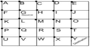
Figure 1. A square-based WSN topology
The figure 1 above illustrates an example of sensor network consisting of 25 nodes named from A to Y arranged in a squared grid based network topology. In this network, node G is designated as source and node Y acts as the sink/destination. The routing scenario where a node cannot forward a message to the node it received the packet from will be assumed. So, only the source node will have four neighbors to select from, and the rest of the nodes along the path will have only three neighbors to choose from as long as they are not border nodes. Therefore it is fair to assume that on an average all nodes will have three neighbors to select from.
In a squared grid based network topology, the expression for the relationship between the boundary nodes and the total number of nodes can be developed as given below. Let the total number of nodes in the grid be represented as
∗
and the number of boundary nodes be represented by b. Then the total number of boundary nodes in any given square grid can be written as:2
2
4
4
( 1 ) Then the ratio between the boundary nodes and the total number of nodes is∗ ( 2 ) The decimal value 4 can be ignored as
→ ∞
lim
→→ 0
( 3 ) Hence it is reasonable to assume that the non-boundary nodes are negligible as the grid gets larger.In figure 1 if node G sends a packet to either F or B it is in the wrong direction, whereas if it sends to either H or L it is in the correct direction towards the sink Y. Using this condition we can calculate the probability of a data packet being successfully sent from node G to the sink node Y. The sink node Y is six hops away from the source node G.
In this scenario it will be assumed that all the neighbors have equal chances of sending or receiving from a neighbor. Therefore the chances of selecting any of the three neighbors are the same. The probability that a packet is forwarded in the wrong or correct direction depends on whether a forwarding node has received the packet from the wrong or correct direction.
For the packet to be successfully routed from node G to node Y, using the shortest path over six hops, it must be forwarded in the right direction for all the hops. The probability that this happens is calculated as follows. If a node received a packet from a correct direction then the probability of forwarding in the correct direction is calculated as follows. A node has three neighbors to select as next-hop. Two of these neighbors are in the
correct direction and have a probability of for forwarding in the correct direction while the remaining
neighbor is in the wrong direction and has a probability of for forwarding in the correct direction. At the initial stage when a neighbour has three messages to send, BREERA will first pick one of its neighbours at random and will forward the first message. For the second message it will pick one of the other two neighbours as the next-hop while the last message is sent to the remaining neighbour. This process is repeated for every three messages a node has to send. Hence the total probability of forwarding a packet in the correct direction
when it has been received from the correct direction is the average of the three neighbors’ probabilities
.
.
.
. If the packet is received from the wrong direction then two of its neighbors are in the wrong direction and only one neighbor is in the correct direction. The two neighbors in the wrong direction have aprobability of each of forwarding in the correct direction while the remaining neighbor is in the correct
forwarding a packet that’s received from the wrong direction to the correct direction is
.
.
.
. If a node received a packet from a correct direction then the probability of forwarding in the correct
direction is and the probability of forwarding in the wrong direction is . On the other hand if a node
received a packet from a wrong direction then the probability of forwarding in the correct direction is and the
probability of forwarding in the wrong direction is .
If the packet is to be forwarded at six hops to reach the destination along the shortest path then it must be forwarded to the correct path in six hops and to the wrong path in zero hops. The probability of this happening is shown below:
6
0.029401
( 4 )Where p is the probability that a packet is forwarded and d is total number of hops the packet travels. However, it is very likely that the packet will not be forwarded to the shortest path by random walk. Therefore it is likely that the packet will be forwarded in the wrong direction before getting to the destination. If the packet is sent one hop in the wrong direction it must move one hop backward towards the correct direction. Therefore, for every one hop in the wrong direction two hops must be added to d to get the total number of hops to route the packet to the destination. In this case where the destination is six hops away from the source, if the packet is forwarded one hop in the wrong direction, then the least number of hops to send it back to the destination would be 8. Therefore, the relationship between the total numbers of hops a packet traverses and the number of hops it traverses in the wrong direction is given as:
2.
, ( 5 ) Where d is the total number of hops a packet travels, k the shortest number of hops between the source and destination and i the number of hops the packet is forwarded in the wrong direction. In the above example k = 6, d = 6 + 2.i. and ‘i’ must be zero and therefore if the total number of hops (d) is six, the packet was forwarded in the correct direction all the time. With the total number of hops being 8, the packet would have been forwarded 7 hops in the correct direction and one hop in the wrong direction. Similarly for d=10, the packet would have been forwarded 8 hops in the correct direction and two hops in the wrong direction. This can be used to easily calculate the probability of successful transmissions at any total number of hops. The probability of successful transmissions at 12 hops is shown below:12
.
.
.
.
.
( 6 )Therefore the probability of a packet reaching the destination at any given number of hops d in scenario 1 can be written as:
2
2
2
.
5
9
2
.
4
9
.
.
.
( 7 )2
2
.
5
9
2
.
4
9
.
.
.
( 8 )Hence the probabilities for successful transmission with 6, 24, 40 and 50 hops are calculated by substituting these values for H and substituting k by 6 as in our example as follows:
6
0.02940119411
( 9 )24
0.7401902058
( 1 0 )30
1.014642274
( 1 1 )In equation 12 it can be seen that the successful transmission probability was more than 100%, this is the result of assuming all the nodes were non-boundary nodes. Hence it can be deduced from the above calculation that, using the proposed biased random algorithm BREERA, it has been proved that it guarantees 100% of the packets to be successfully transmitted using the same energy (30e) as the spf algorithm.
The spf routing requires 5k energy cost as calculated above. In [6] it is found that flooding algorithm requires 2m (m – 1) energy cost in a WSN with a grid size of m * m, m being the number of nodes in each edge. Figure 2 compares the energy cost of these algorithms by routing messages on the longest path in the grid (k = 2(m-1)).
Routing Algorithm Number of hops Energy cost
Shortest path k 5k
BREERA 5k = (5*6) with
100% successful transmission rate
5k
Flooding K(k/2-1) K(k/2-1)
Figure 2 Performance comparison of spf, flooding and BREERA
5. Empirical Analysis of BREERA
An experimentation using a small grid size of 5 x 5 sensor nodes has been conducted on the proposed routing algorithm in order to evaluate its effectiveness and to compare with its statistical analysis. This experiment is also intended to explain the working mechanism of the proposed routing algorithm. It demonstrated how the node counters are generated and how they are used in selecting the next hop node. In experiment 1 all the information is given as an example but for experiment 2, 3 and 4 only the results are shown and analyzed. The network scenario illustrated in figure 1 is considered for the experimentation.
BREERA algorithm:
1. To select the next hops, a node checks its counters and forwards to the neighbor with the smallest number of entries which means the one with the highest energy
2. When two or more values are equal then a die is cast. A result of 1, 2, 3 or 4 will forward the packet to the right, up, left or down direction of the forwarding node to the next hop respectively.
3. A packet received is represented by a ‘0’ while a packet sent is represented by a ‘1’ in the corresponding energy counter
4. A packet received is evaluated as equivalent to 4 packets sent while comparing the counters for forwarding decision
5. In each experiment 24 messages are routed from source to destination following the above rules.
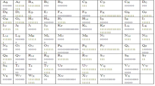
Experimental scenario 1: In this experiment the source node is G and the destination node is Y. This experiment is used to test the algorithm for a common situation in WSNs where, an intermittent activity happening within an area needs to be reported back to the sink. The node energy counters are shown in figure 3 below for this experimental scenario.
Figure 3. Node counters for experiment 1
The events are packets being sent from source to destination following the above mentioned rules. There are 24 events but only 2 of them will be demonstrated here. The data generated from these events is used to fill the counters. This is illustrated in figure 4.
Figure 4. Packet flow
Figure 5. Energy used by the nodes for sent and received packets when using BREERA algorithm for experiment 1.
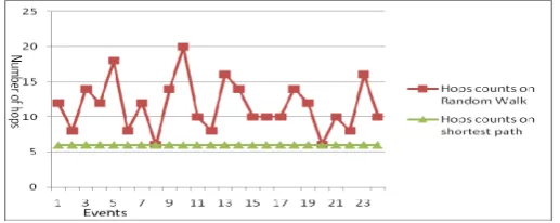
Figure 5 gives the values for all the packets sent and received in the grid which in turn represent the energy used in the network. The total energy used by the network in experiment 1 while employing BREERA algorithm was 532 units of energy. The maximum energy used by a node was 44 units of energy while the smallest was 4 units of energy. The mean energy used was 22.2 with a standard deviation of 9.1 units of energy. All the nodes participated in forwarding the packets to the sink. However for the shortest path 720 (5 *6*24) units of energy would have been used to send the packets to the destination. With shortest path all these packets would have been sent using the same 6 nodes along the shortest path to the destination. This would have meant that the average energy used by each of these nodes would have been 120 units of energy. If the nodes’ initial energy were 100 units each, then all the 6 six nodes would have depleted their energy before the 24 transmission were completed and hence partitioning of the network would have occurred. Figure 6 shows the average number of hops used by both BREERA and SPF algorithms for each event.
Figure 6. Average Hop Counts for BREERA algorithm in experiment 1
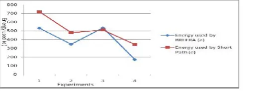
Experimental scenario 2: The source is node G and the destination node S which is closer to the centre is selected for demonstration in this experimentation. This is to study the behavior of the algorithm when the sink is placed closer to the middle of the grid. The data obtained from the 24 events is analyzed as shown below. The total energy by the BREERA algorithm in this experimental scenario was 347 units as shown in figure 7. The maximum energy used by a node was 29 units of energy while the smallest was 2 units of energy. The mean energy used was 14.5 with a standard deviation of 7.2 units. All the nodes participated in forwarding the packets to the sink. However for the shortest path 480 (4 *5*24) units of energy would have been used to send the packets to the destination. With shortest path all the packets would have been sent using only the 4 nodes along the shortest path to the destination. This would mean that the average energy that would have been used by each of these nodes would have been 120 units. If the node’s initial energy was 100 units then all the 4 nodes would have been depleted of their energy and hence partitioned the network sooner.
The total energy used by BREERA algorithm was 535 units as shown in figure 7. The maximum energy used by a node was 38 units of energy while the smallest was 9 units of energy. The mean energy used was 22.3 with a standard deviation of 8.3 units of energy. All the nodes participated in forwarding the packets to the sink. However for the same scenario, the shortest path algorithm would have used 510 (5 *102) units of energy to send the packets to the destination.
Experimental scenario 4: The source is selected at random and the destination node S is at the centre of the grid. This is to study the behavior of the algorithm when the sink is placed at the centre of the grid.
The total energy consumed by the network while employing BREERA was 171 units of energy as shown in figure 7. The maximum energy used by a node was 16 units of energy while the smallest was 1 unit of energy. The mean energy used was 7.1 with a standard deviation of 4.0 units of energy. All the nodes participated in forwarding the packets to the sink. However for the shortest path algorithm 345 (5 *69) units of energy would have been used to send the packets to the destination as shown in figure 7.
Figure 7 Results from the experiments 1 to 4, showing the comparison of energies used by the sensor network when using shortest path routing and BREERA algorithms
6. Conclusion
In this research paper, a novel routing algorithm named BREERA has been proposed. This protocol works on a squared grid based network topology and is suitable for applications whereby the data to be sent is small enough to be compared with the exchange of information between neighboring nodes. For these applications such as environmental monitoring and danger alarm monitoring it has been statistically and empirical proved that BREERA consumes much less amount of energy when compared to the shortest path first routing algorithms. Further investigation is required on a wider range of scenarios in order to establish the efficiency of BREERA and to define the trend in power consumption in various network scenarios. In the experiments considered above, it was shown that the further the node is from the sink the more efficient the packet is in reaching the sink. The assumption made at the beginning of the discussion; that a received message counts as four sent message makes the nodes to get a sense of the direction of the Sink has been empirically justified. These findings suggest that BREERA is tunable and the best way to further justify this is through a large number of simulations on a range of network scenarios which is currently being carried out by the researcher.
References
[1] F. Akyildiz, S. Weilian, Y. Sankarasubramaniam, and E. Cayirci, "A survey on sensor networks," Communications Magazine, IEEE,
vol. 40, pp. 102-114, 2002.
[2] C. De Morais Cordeiro and D. P. Agrawal, Ad hoc & sensor networks : theory and applications. Hackensack, NJ: World Scientific
Publishing Co., 2006.
[3] R. Beraldi, R. Baldoni, and R. Prakash, "Lukewarm Potato Forwarding: A Biased Random Walk Routing Protocol for Wireless Sensor
Networks," in Sensor, Mesh and Ad Hoc Communications and Networks, 2009. SECON '09. 6th Annual IEEE Communications Society Conference on, 2009, pp. 1-9.
[4] D. Vergados and N. Pantazis, "Energy-Efficient Route Selection Strategies for Wireless Sensor Networks," Mobile Networks and
Applications, vol. 13, pp. 285-296, 2008.
[5] G. Xin, L. Guan, X. G. Wang, and T. Ohtsuki, "A Novel Routing Algorithm Based on Ant Colony System for Wireless Sensor
Networks," in Computer Communications and Networks, 2009. ICCCN 2009. Proceedings of 18th Internatonal Conference on, 2009, pp. 1-5.
[6] T. Hui, S. Hong, and T. Matsuzawa, "RandomWalk Routing for Wireless Sensor Networks," in Parallel and Distributed Computing,
Applications and Technologies, 2005. PDCAT 2005. Sixth International Conference on, 2005, pp. 196-200.
[7] H. Shokrzadeh, A. T. Haghighat, F. Tashtarian, and A. Nayebi, "Directional rumor routing in wireless sensor networks," in Internet,
2007. ICI 2007. 3rd IEEE/IFIP International Conference in Central Asia on, 2007, pp. 1-5.
[8] M. Jiang, J. Li, and Y.C. Tay, "Cluster Based Routing Protocol functional specification," IETF Internet Draft, 1998.
[9] S. Meguerdichian, F. Koushanfar, M. Potkonjak, and M. B. Srivastava, "Coverage problems in wireless ad-hoc sensor networks," in
[10] S. Zhen-wei, Z. Yi-hua, T. Xian-zhong, and T. Yi-ping, "An Ant Colony System Based Energy Prediction Routing Algorithms for Wireless Sensor Networks," in Wireless Communications, Networking and Mobile Computing, 2008. WiCOM '08. 4th International Conference on, 2008, pp. 1-4.
[11] F. Ye, A. Chen, S. Liu, and L. Zhang, "A scalable solution to minimum cost forwarding in large sensor networks," In Proceedings of
the tenth International Conference on computer Communications and Networks (ICCN), pp. 304-309, 2001.
[12] K. K. Rachuri and C. S. R. Murthy, "Level Biased Random Walk for Information Discovery in Wireless Sensor Networks," in In
Proceedings of the 2009 IEEE international conference on Communications (ICC), 2009, pp. 1-6