INTELLIGENT CONTROL USING
ADAPTIVE PID CONTROLLER
DR. P VIJAYAKUMAR
Vice principal, Kathir College of Engineering , Anna University, Neelambur, Coimbatore-641 062, TN, India
UNNIKRISHNAN P C
Research Scholar, EEE Department, Karpagam University, Eachanari Post, Coimbatore-641 021, TN, India
[email protected] Abstract:
In this paper an adaptive stable PID controller is briefly explained and validated by simulations and experimentation. The adaptive PID controller employs almost strict positive realness (ASPR) to ensure stability of the system. The design involves a parallel feedforward compensator (PFC) which guarantees the ASPRness of the controlled system. After a disturbance the dynamical system is assumed to be in one of a finite number of configurations, corresponding to each of which exist a stabilizing controller. The effectiveness of the method is tested and compared using simulations and experiments on a level control experimental setup.
Keywords:Adaptive PID Controller, Parallel Feedforward Compensator, Neural Network Controller, Fuzzy logic Controller.
I. Introduction
PID controllers are widely used in process industries. Selecting the right proportional, Integral and derivative settings on-line is a real challenge. Automatic tuning and stabilizing of PID controllers have been a topic of great significance over the past many years [1]. PID control system involves complex stability problem due to the lack of sufficient number of tuning parameters compared to the order of the plant. Therefore it is important to consider the problems of auto-tuning of near optimal PID controllers and their stability with the three adjustable parameters namely Proportional, Integral and Derivative. Auto-tuning of controller is explained in detail in the book by Astrom and Hagglund [2]. Recent research works in similar fields are Self-tuning approach [3][4], standard relay feedback and auto-tuning using neural networks [5],[6],[7][8], stochastic divergence optimization method [9], Fuzzy self tuning controllers [10][11], and reinforcement learning algorithm [12]. In this paper we look at a simple PID controller where the process is ASPR (Almost strict positive realness). It has been proved that a linear time invariant (LTI) system can be stabilizable by output feedback, if the controlled plant is ASPR [13]. This novel PID controller always ensures stability so that we don’t have to worry about the stability regions. The effectiveness of this method is tested by simulations and experimentation on a non-linear level control system approximated to a first order system with time delay.
II. Stable PID Controller
An adaptive stable PID controller is briefly explained here. For a rigorous analysis and proofs please refer to the article by Shah S.L. et al [14].
A. Problem Setup
Consider the following controllable and observable SISO nth order plant:
1 1
, , ,
) ( ) (
) ( ) ( ) ( ) (
R d y u R x
t x c t y
t d b t bu t Ax t x dt
d
n T
(2.1)
Where d(t) denotes the disturbance input. The transfer function of 2.1 is expressed by
) (
) ( )
( )
( 1
s D
s N b A sI c s G
p p
T
(2.2)
Equation 2.1 is said to be ASPR if there exists a feedback gain ke such that the system defined by (A- kebcT, b,c) is SPR. [15][16].
B. Extended plant model
An extended plant model is introduced which includes tracking error in the equation. Let us define z(t), v(t) and the tracking error e(t) as follows.
) ( ) ( ) ( ) ( ) ( ) ( ) ( ) ( ) ( t r t y t e t u s D t v t x s D t z (2.3)
which leads to the following equation
D(s)e(t) =cTz(t) (2.4)
From 2.1, 2,3 and 2.4 we have the extended plant model:
) ( ) ( ) ( ) ( ) ( t x c t y t v b t x A t x dt d T (2.5)
where v(t) is the input and y(t)is the output of this system. The Transfer function of the extended model is given by ) ( ) ( 1 )
( G s
s D s
GP (2.6)
C. Introduction of PFC
In 2.5 , cTb0 holds. (2.7)
It means that the relative degree of 2.6 is not ASPR [17]. A parallel feedforward compensator (PFC) is introduced to improve the situation
0 ) ( ) ( ) ( ) ( ) ( f T f T f f f f f f b c t x c t y t v b t x A t x dt d (2.8)
Combining 2.5 and 2.8, we get the model of the extended plant with PFC
) ( ) ( ) ( ) ( ) ( ) ( ) ( t x c t y t y t y t v b t x A t x dt d T a f a a a a a (2.9) Where f a f a f a f a c c c b b b A A A x x
x 0 , ,
0 ,
The corresponding transfer function is given by
Ga(s) = GP(s) + GPFC(s) (2.10)
where GPFC(s) denotes the transfer function of the PFC. D. Adaptive PID Controller
Since the extended plant with PFC is ASPR, it can be stabilized by using the following Adaptive controller [14]
0 , 0 , 0 , ) ( ) ( * * 10 3 * * * * *
i d p a i a d a p k k k k where dt t y k t y dt d k y k v (2.11)
() , () ), ( ) ( )] ( ), ( ), ( [ ) ( ) ( ) ( ) ( t y dt d dt t y t y t z t k t k t k t k t z t k t v a a a T d i p T T T (2.12)The adaptive PID gain vector k(t) is tuned based on the adaptive tuning rule:
0 ) ( ) ( ) ( T a t y t z t
k (2.13)
Other adaptive parameter laws also can be used. The parameter estimation error converges to zero if the regression vector z(t) includes sufficiently rich frequencies.
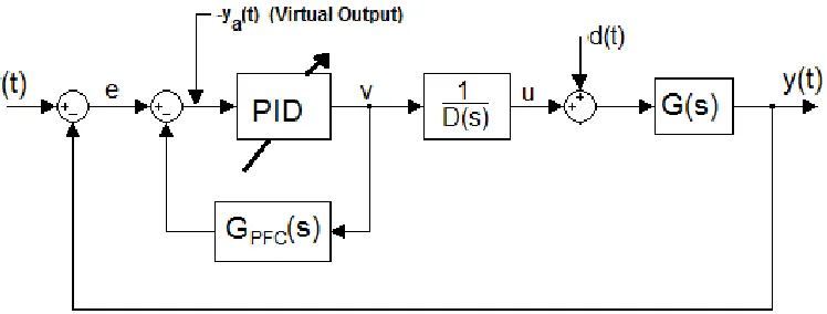
Figure 1. Block diagram of Adaptive PID Control system III PFC Construction using Approximated plant model
A. Structure of PFC
Many methods have been proposed in the past to the design of PFC [16]. A ladder network type PFC has a simple structure and commonly used [18]. This network requires the knowledge concerning the relative degree and the minimum phase characteristics of the plant. An approximated plant model for PFC construction is relatively simple and easy [14].
Let G*(s) be an approximate model of G(s). Then G*P(s)is defined as
) ( ) ( 1 ) ( *
* G s
s D s
GP
Let GASPR(s) be an ASPR transfer function which is indicated by designers. Then we construct PFC as follows
) ( ) ( )
(s G s G* s
GPFC ASPR P (3.1)
Hence, )) ( 1 )( ( ) ( ) ( ) ( ) ( ) ( ) ( * s s G s G s G s G s G s G s G ASPR P ASPR P PFC P a (3.2)
Where (s)GASPR(s)1(Gp(s)Gp*(s)) (3.3) The extended system (3.2) becomes ASPR if the following conditions are satisfied.
(1) GASPR(s) is ASPR
(2) (s)RH (3.4)
(3) (s) 1 (3.5)
Suppose that PFC has the form shown in 3.1 and 3.4 holds. Further suppose that adaptive parameters reach to some constant values at the steady state. Then if r(t) and d(t) are step functions and
(1) GPFC(0) = 0,
(2) G(0) ≠ 0 and ki0, then we have
0 ) ( lim )) ( ) ( (
lim
y t rt t et
t (Ref [6] for Proof) (3.6)
IV. Application to the Control of a Level Control System
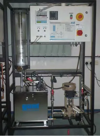
The effectiveness of the method discussed is tested by MATLAB simulations with the non-linear level control system approximated to a first order system with time delay. The level control systemexperimental set-upis shown in figure 2and is available in the process control lab of Al Musanna College of Technology, Sultanate of Oman. The system involves a water tank (System), PID controller, water pump and a pneumatically controlled valve. The pneumatic valve can be replaced by a solenoid valve. The system can also be controlled using a computer connected to it. Results of simulation are compared with experimental results.
Figure 2. Level Control System Experimental Set-up A. Simulation
In the case of a level control system, the transfer function between input (Set-point or disturbance) and water level of the tank (output) can be approximated by a first order plus time delay model [2][19]. Many PID controller parameter tuning rules have been proposed when the process can be approximated as in the form 4.1 [19]. In this example, plant model 4.1 is used as a test model of the PID controller. Further, we assume that the set point and the disturbance input are step inputs because many actual systems can be modeled by 4.1 and PID tuning algorithm methods are based on step variations in set point and disturbance inputs.
(1) Plant model
Ls e Ts
K s
G
1 )
( (4.1)
(2) Set Point and disturbance model:
As both Set Point and disturbance inputs are step inputs
D(s) = 1 (4.2)
(3) Approximate Plant model
To design PFC, the time delay is approximated by the simple 0/1-order Pade-approximation:
LS e Ls
1
1
(4.3)
) 1 )( 1 ( ) ( *
Ls Ts
K s
G
(4) PFC
) ( ) ( )
(s G s G* s
GPFC ASPR P
Where
1 ) (
s s ASPR
T K s G
(5) Adaptive parameter adjusting law
The control input is given by [2.12] with the parameter adjusting law [2.13]. (6) Basic Simulation data:
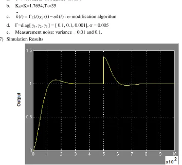
a. T=74.4782, L=16.9226,K=1.7654 b. KS=K=1.7654,TS=35
c. k(t)z(t)ya(t)k(t)
: -modification algorithm d. =diag[ 1, 2, 3 ] = [ 0.1, 0.1, 0.001], = 0.005 e. Measurement noise: variance = 0.01 and 0.1. (7) Simulation Results
Figure 4. Simulation Result: Output of the plant with measurement noise (Variance = 0.1)
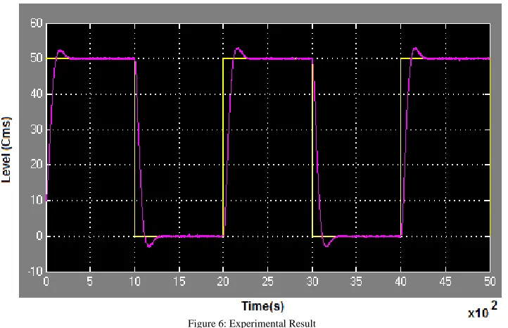
B Experimental Result
Figure 6: Experimental Result
The experimental result of the level control system is shown in Figure 6. This experimental set-up is available in the process control lab of Al Musanna College of Technology, Sultanate of Oman. A picture of the experimental set-up is shown in Figure 2. Actual control input is the water flow rate and the output is level of water. All controller parameter values and reference input are the same as those of the parameters and reference input used in the above simulation. The result of the simulation is given in Figure 4. The variation in the output response in the experimental setup and simulation is attributed by the response of the pneumatically controlled valve. The output variance can be reduced by introducing proper filters and the response can be made faster by using solenoid valve. These experimental modifications are left for future activity.
V. Conclusion
In this paper, an adaptive stable PID control design scheme based on the ASPRness of the plant is discussed and applied to a first order system with time delay. The effectiveness and robustness of the design is validated by simulation and experimentation on an experimental level control system.
References
[1] Åström, K. J., et al. "Automatic tuning and adaptation for PID controllers-a survey." Control Engineering Practice 1.4 (1993): 699-714.
[2] Astrom, K.J. and T Hagglund , PID Control, theory, Design and Tuning, Instrument Society of America, USA, 2006.
[3] Arrieta, O., A. Visioli, and R. Vilanova. "PID autotuning for weighted servo/regulation control operation." Journal of Process Control 20.4 (2010): 472-480.
[4] Leva, A., Negro, S., & Vittorio Papadopoulos, A. (2010). PI/PID autotuning with contextual model parametrisation. Journal of Process Control, 20(4), 452-463.
[5] Ohnishi,Y., T.Yamamoto and S. Ohmatsu, A Design of Multivariable self-tuning PID controllers with an internal model structure, Electrical Engineering in Japan, Vol. 146, No. 4, pp. 58-64, 2004.
[6] Hang, C.C., K.J.Astrom and Q.C.Wang, Relay feedback auto-tuning of process controllers- a tutorial review, J. of Process Control, Vol. 1 2, pp.143-162, 2002.
[7] Chang, Whan.D., R.C. Hwang, J.G. Hsieh, A multivariable on-line adaptive PID controller using Auto-tuning Neurons, Engineering application of Artificial Intelligence, Vol. 16, pp. 57-63, 2003.
[8] Kaur, Japjeet, et al. "Speed Control of Hybrid Electric Vehicle Using Artificial Intelligence Techniques." Int. J. Net. Tech. Sys 2.1 (2014): 33-39.
[9] De, Ritu Rani, and Rajani K. Mudi. "Fuzzy Self-tuning of Conventional PID Controller for High-Order Processes." Proceedings of the International Conference on Frontiers of Intelligent Computing: Theory and Applications (FICTA) 2013. Springer International Publishing, 2014.
[10] Saad, Mohd S., Hishamuddin J., and Intan Z.D., "PID Controller Tuning Using Evolutionary Algorithms.", Wseas transactions on Systems and Control, Issue 4, Volume 7, 2012.
[11] Mudi, Rajani K., and Ritu Rani De Maity. "A Noble Fuzzy Self-Tuning Scheme for Conventional PI Controller." Proceedings of the International Conference on Frontiers of Intelligent Computing: Theory and Applications (FICTA). Springer Berlin Heidelberg, 2013. [12] Shang, X. Y., et al. "Parameter optimization of PID controllers by reinforcement learning." Computer Science and Electronic
Engineering Conference (CEEC), 2013 5th. IEEE, 2013.
[13] Roy, A. and K. Iqbal, Synthesis of stabilizing PID controllers for bio-mechanical models, Proceedings of IFAC World congress, Praha, 2005.
[14] Shah S.L.,Jiang H., Iwai Z et al., Adaptive Stable PID controller with Parallel Feedforward Compensator, IEEE, 2006.
[16] Kaufman, H.,I. Bar-Kana and K. Sobel , Direct Adaptive Control Algorithms, Theory and applications, Springer-Verlag,USA, 1994. [17] Roy, A. and K. Iqbal.Synthesis of stabilizing PID controllers for biomechanical models, Proceedings of 2005 IFAC World Congress,
Praha.
[18] Iwai,Z., and I.Mizumoto,Realization of simple adaptive control by using parallel feedforward compensator, Int. J. Control, Vol.59, No. 6, pp. 1543-1565, 1994.