PERFORMANCE STUDY OF TOOL
MATERIALS AND OPTIMIZATION OF
PROCESS PARAMETERS DURING EDM
ON ZrB
2
-SiC COMPOSITE THROUGH
PARTICLE SWARM OPTIMIZATION
ALGORITHM
S.SIVASANKAR
Research Scholar,
Department of Production Engineering, National Institute of Technology,
Thiruchirappalli-620015, Tamilnadu, India
E-mail:[email protected]
R.JEYAPAUL
Associate Professor,
Department of Production Engineering, National Institute of Technology,
Thiruchirappalli-620015, Tamilnadu, India E-mail:[email protected] Abstract:
This paper deals with optimization of EDM of ZrB2-SiC composite using Particle swarm optimization (PSO). In this work ZrB2 with different volume proportions of SiC (15, 20, 25 and 30%) are selected as workpiece. ZrB2– SiC ultra high temperature ceramics exhibited an excellent thermal-oxidative and configurationally stable under supersonic conditions, which suggests they are potential candidates for leading edges. Results indicate that ZrB2–SiC can maintain the high oxidation resistance coupled with configurationally stable at temperatures lower than that point which results in significant softening and degradation of the oxide scale, and that point will be the temperature limit for UHTC.It is a candidate for high temperature aerospace applications such as hypersonic flight or rocket propulsion systems. To expand its area of applications, machining is mandatory. Due to high strength and hardness of ZrB2 mechanical machining is very difficult or even impossible. Electrical discharge machining is promising technology to machine ceramic components of complex shape with high-dimensional accuracy and good surface roughness. In this investigation the influence of SiC over the machinability is carried out. Input parameters are pulse on time, pulse off time and tool materials (graphite, titanium niobium, tantalum and tungsten). Pulse on time and pulse off time are kept at three different levels. Objective is to maximize the material removal rate (MRR) and to minimize the roundness, surface roughness (SR), tool wear rate (TWR), Overcut and taper angle during EDM of hot pressed ZrB2-SiC composite. In general Desirability Functional Analysis (DFA) is used to combine multiple quality characteristics into a single performance statistics. While combining the quality characteristics, weight should be assigned to each response. For this problem, unequal weights are assigned using particle swarm optimization (PSO). Interaction of pulse on time with tool material is investigated using analysis of variance (ANOVA) and it shows that tool material is most significant factor. Keywords: roughness,roundness,taper angle,overcut,ZrB2,SiC,PSO,DFA,Ceramics,Composite.
1. Introduction
Luigi Scatteia, 2008). The high electrical conductivity of ZrB2 (108 S/m) is sufficient for electrical discharge machining (EDM) allowing for relatively low cost machining of complex components (Cutler R. A, 1992). Since the ceramic materials possess exceptional mechanical and chemical properties such as high compression strength, high hardness, low ductility, high corrosion resistance, low specific weight, and a high strength even at very high temperatures (Klocke F, 1997) they have a wide range of applications. The typical processes of engineering ceramic components are compacting techniques of powder metallurgy and high-temperature sintering. However, ZrB2 is not only hard to sinter [1,2], but also by itself does not meet all the exigent requirements of oxidation resistance and mechanical properties demanded by extreme-environment aerospace engineering [1,2]. For these reasons, ZrB2 is typically combined with other refractory ceramics. One of the most widely used is SiC at relative concentrations between 5 and 30 vol.% [1,2]. Chamberlain et al. (2004) reported the flexural strength increased from 550 MPa for pure ZrB2 to 1100 MPa for ZrB2–30 vol% SiCp. Likewise, fracture toughness ranged from 3.5 to 5.3 MPa m1/2 over the same composition range. Meanwhile, Hwang et al (2007) studied the properties of ZrB2–SiC composites as a function of SiC grain size. Results showed that a reduction in the SiC grain size can improve the processing and oxidation resistance of ZrB2–SiC composites.Monteverde and Bellosi [11,12] also found that ultra-fine SiC particulates could improve the sinterability and mechanical properties of ZrB2 and a mixture of ZrB2 and HfB2.Monteverde F et al (2006) documented that ZrB2 and HfB2 can be strengthened and toughened through the incorporation of SiC particles. Therefore, ZrB2 based and HfB2 based composites reinforced by SiC particles have been investigated by many researchers. Producing complex shapes such as holes, internal cavity in ceramics with high dimensional accuracy is very difficult to achieve through these conventional machining techniques and they are expensive to produce. The use of traditional cutting machinery to machine hard and brittle ceramic materials can cause cracks on the machined surface (Allor RL and Jahanmir S, 1996). Electric discharge machining (EDM) is the best choice for the manufacture of conductive ceramic materials because there is no contact between the tool and workpiece during the EDM process. In the EDM process, the surface layer of a workpiece can be rapidly melted and removed by an arc of 8,000 –12,000°C at each charge point. EDM takes advantage of spark-erosion manufacturing to machine the hard to cut material which efficiently produces the required shapes and sizes, finer surface characteristics, and better dimensional accuracy. Over the past few years, EDM has been widely applied in the modern metal industry for producing intricate and complex shapes required for conductive ceramic materials that are difficult to manufacture by conventional machining (Mc Geough JA, 1988).
Selection of tool material for machining the ceramic is the major area to be analyzed since electrode wear occurs during EDM process leading to a lack of machining accuracy in the geometry of workpiece. To reduce the influence of the electrode wear, it is necessary either to feed electrode larger than the workpiece thickness in the case of making through-holes, or to prepare several electrodes for roughing and finishing in the present state of technology. Very few literatures are available on tool material performance evaluation. Yao-Yang Tsai stated that volumetric wear ratio of the electrode becomes small for the electrode material with high boiling point, high melting point, and high thermal conductivity. This tendency is independent of the workpiece materials. An index is proposed to include the boiling phenomenon for evaluating the erosion property of electrode material in EDM (Yao-Yang Tsai, and Takahisa Masuzawa, 2004) The effects of electrode tool materials and machining input parameters on AISI D3 EDM characteristic, by the use of variance analysis and experiments designing techniques is studied and reported that the graphite electrode, having highest material removal rate and precise dimension and low tool wear ratio, is the most appropriate material for steel machining (Khoshkish, Ashtiani, Goreyshi).
R.A. Mahdavinejad studied about the machining of carbon-based materials such as WC-Co and non-oxide ceramics, which are growingly used and it’s the complexity and non-linear nature of EDM. For getting the instantaneous data from machining condition, the new method of fuzzy analysis of single machining pulses and computing the magnitude of system condition in the form of a real number between 0 and 1 has been used. Some tests with WC-Co material are carried out and finally, the results of implementation of control system on a sinking ED machine and an EDM system that has been set and it has been compared (Mahdavinejad R.A, 2009).
Particle swarm optimization (PSO) is an evolutionary optimization technique that simulates the social behavior of bird flocking to desired places (Eberhart R.C. and Kennedy J, 1995; Kennedy, J and Eberhart R.C, 1995). PSO starts by initializing a population of random solutions and searches for optima by updating generations. PSO does not use any evolution operators. In PSO, particles fly through the problem space by following its own experience and the best experience attained by the swarm as a whole (Andreas C.Nearchou, 2011). In contrast to analytical or general heuristic methods, PSO is computationally efficient and has great capability of escaping local optima PSO was originally developed by Kennedy and eberhart in 1995, it is a population-based evolutionary algorithm.
PSO is initialized with a population of random solutions (particles) using uniform distribution. Each particle in PSO traces a trajectory in an n-dimensional search space, updating constantly a velocity vector based on best solutions found so far by that particle as well as others in the population (swarm). Each particle keeps track of its coordinates in the problem space, which are associated with the best solution (fitness) it has achieved so far, Pbest. Another ‘‘best” value tracked by the global version of the particle swarm optimizer is the overall best value, Gbest, and its location, obtained so far by any particle in the population. The particle swarm optimization algorithm, at each time step, changes the velocity of each particle moving towards its Pbest and Gbest locations. Velocity is weighted by random terms, with separate random numbers being generated for acceleration toward Pbest and Gbest locations, respectively (Ritchie Mae gamut and armacheska mesa, 2008; Thakshila,Wimalajeewa and Sudharman K. Jayaweera, 2007; Hong Zhang, Heng Li and C.M. Tam, 2006).
The objective of this work is to study the influence of pulse duration during EDM of hot pressed ZrB2-SiC composite and also to identify the best suited tool material for the selected work piece. In this work, roundness, roughness, MRR, TWR, overcut and taper angle are considered as the responses. These multi responses are combined into single response problem using DFA. For this problem, weights are assigned using PSO and interaction of Pulse on time with tool material is investigated using ANOVA.
2. Experimental set-up and method
2.1 Tool material
Graphite (GR), Titanium (Ti), Niobium (Nb), Tantalum (Ta), Tungsten (W), is selected as the tool materials. Cylindrical electrodes of 2 mm diameter from these materials were fabricated through different techniques like wire cut EDM, Diamond grinding and Extrusion process.
2.2 EDM machine specifications
Electronica small sinker machine of series 500 x 300 was used for experimentation. The specification of this machine is Max working current is 35A, Work table size is 500 x 300mm, Power supply is 3 phase, 415VAC, 50Hz. Table 1 gives the details of experimental conditions.
Table.1.Experimental conditions ____________________________________________________ Dielectric medium Kerosene
Polarity Tool: Negative
Workpiece: Positive
Open circuit voltage 100V Discharge current 2A
Pulse on 4µs, 7µs, 10µs Pulse on 1µs, 3µs, 5µs Workpiece dimension 65 x 65 x 4.2 mm Tool diameter 2mm
Dielectric medium Kerosene
2.3.0 Design of Experiments
2.3.1 Material Removal Rate (MRR)
Material removal rate is the volume of material removed from the workpiece per unit time. It is calculated by measuring weight of workpiece before and after machining, and machining time .MRR is calculated based on the following relation.
M A B
T W W
MRR
2.3. 2.Tool Wear Rate (TWR)
Tool wear rate is the volume of material removed from the tool per unit time. It is calculated by measuring
weight of tool before and after machining, and machining time.
M A B
T w w
TWR
2.3.3 Roughness
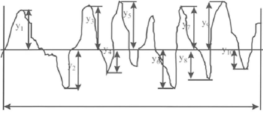
The surface roughness is assessed by peak-to-valley heights (Rmax) of the craters. the surface roughness were found using video measuring machine (ARCS, Model KIM1510) and image processing using Mat lab. For roughness the hole is cut in half along the axis. Then the image is taken using video measuring machines. Peak to peak height is defined as the height difference between the highest and lowest pixel in the image. Peak to peak height was measured using Ten Point Height, where the difference of the five high local maximums and five low local minimum in a continuous sample length. Ten Point heights were got by selecting a sample length of relative a linear path (C h a n g , H . , L i m , T . V , 1 9 9 3 ) .
(1)
Where ypi are the most important five upper points(y1, y3, y5, y7, y9) and yvi are the most important five lower points of the profile (y2, y4, y6 ,y8 , y10) and shown in Fig.1. Fig.2 shows the display of the matlab output during roughness measurement.
Fig. 1. Ten point roughness measurement Table 2 Design of experiments
Factor/Level 1 2 3 4 5
A. Tool Graphite Titanium Niobium Tantalum Tungsten
B. Pulse on (µs) 4 7 10 - -
C. Pulse off (µs) 1 3 5 - -
D. Work piece(No) 85%ZrB2 -15%SiC (1)
80%ZrB 2 -20%SiC (2)
75%ZrB 2 -25%SiC(3)
70%ZrB 2
-30%SiC (4) -
Where wB =Weight of the tool before machining wA=Weight of the tool after machining
Fig.2.Mmatlab output during roughness measurement
2.3.4 Roundness
Fig.3.Image of hole profile
2.3.5 Taper angle
Taper angle is calculated by measuring the top and bottom diameters of the machined hole. Diameters are measured using video measuring machine with matlab.Figure 3 shows the output of the matlab.In this figure the middle circle diameter is the nominal diameter of the hole at the top. Then the procedure is repeated to find the bottom diameter of the hole. Using the following equation the taper angle is calculated.
2.3.6 Overcut
Deviation of hole diameter (middle circle diameter in figure 3) from tool diameter (2mm) is calculated as overcut.
Table.3.Response value
Ex.No Tool Fraction
of SiC
Pulse on time(µ s)
Pulse off time(μs)
MRR TWR
Roughness(µ m)
Roundness(µ m)
Taper
angle(deg) Overcut(mm)
(mg/min) (mg/min)
1 GR 0.15 4 1 1.1311 1.962 6.4615 83.6246 5.6967 0.4527
2 Ti 0.15 4 1 1.9119 5.005 8.4845 86.2683 5.7978 0.2536
3 Nb 0.15 4 1 0.981 6.6767 9.006 100.964 5.6286 0.6547
4 Ta 0.15 4 1 0.8208 6.006 9.1672 86.6406 5.5496 0.6453
5 W 0.15 4 1 0.961 0.1802 4.5936 81.7868 5.4505 0.6167
6 GR 0.15 4 3 0.6807 1.9019 9.96 69.2553 6.042 0.817
7 Ti 0.15 4 3 0.8108 6.006 10.4214 72.3494 6.3834 0.7182
8 Nb 0.15 4 3 0.7107 7.988 8.0801 80.8388 6.014 0.6498
9 Ta 0.15 4 3 0.6607 3.3333 5.2482 70.2493 5.8248 0.6879
10 W 0.15 4 3 0.6206 7.8078 12.1361 278.4384 5.8058 0.6618
11 GR 0.15 4 5 0.5005 1.7918 7.5726 60.8819 7.008 0.8424
12 Ti 0.15 4 5 0.3704 3.5035 12.1181 63.5355 7.5095 0.8435
13 Nb 0.15 4 5 0.3604 1.3313 10.2673 36.2793 6.6396 0.7849
14 Ta 0.15 4 5 0.5706 6.7868 11.98 68.5425 6.4504 0.7851
15 W 0.15 4 5 0.4104 4.5746 5.995 68.2633 6.4114 0.7569
16 GR 0.15 7 1 2.2723 1.6517 9.7097 137.3834 2.3984 0.3152
17 Ti 0.15 7 1 2.2523 0.4605 11.1922 130.988 2.4595 0.3162
18 Nb 0.15 7 1 2.0621 0.6206 9.1211 131.97 2.2502 0.1672
19 Ta 0.15 7 1 0 0 7.6807 128.6376 1.6206 0.1681
20 W 0.15 7 1 0.961 1.5315 9.3734 137.2272 1.0911 0.1692
21 GR 0.15 7 3 1.3514 1.001 8.2733 121.5626 2.984 0.4103
22 Ti 0.15 7 3 0.8108 1.6717 8.5646 126.6987 3.2052 0.4117
24 Ta 0.15 7 3 1.2212 0.2903 9.0871 113.007 2.6767 0.185
25 W 0.15 7 3 1.5315 0.7007 6.4554 121.3764 2.6576 0.1806
26 GR 0.15 7 5 0.7307 0.6707 8.8288 103.5395 3.6797 0.237
27 Ti 0.15 7 5 1.1311 0.4004 6.4374 103.4304 3.7808 0.2383
28 Nb 0.15 7 5 0.4004 3.6737 9.6516 111.3293 3.4114 0.2394
29 Ta 0.15 7 5 0.5506 0.9309 10.2733 106.015 3.3523 0.2406
30 W 0.15 7 5 0.5305 0.1201 5.9699 101.0811 3.2132 0.2413
31 GR 0.15 10 1 1.9319 1.4014 10.6356 444.1051 4.1952 0.2627
32 Ti 0.15 10 1 1.3514 0.951 7.994 220.2222 4.2963 0.2633
33 Nb 0.15 10 1 1.0911 1.2813 11.8588 228.1812 3.9669 0.2445
34 Ta 0.15 10 1 1.982 1.3814 12.0901 412.4664 3.9679 0.2453
35 W 0.15 10 1 1.8218 6.5265 5.8648 490.1852 3.7988 0.2476
36 GR 0.15 10 3 0.9109 1.2513 8.8688 189.8058 4.9309 0.367
37 Ti 0.15 10 3 0.3103 0.2202 5.6466 168.6056 4.992 0.3684
38 Nb 0.15 10 3 0.4705 0.4304 8.5305 189.7577 4.8328 0.339
39 Ta 0.15 10 3 0.4805 0.3504 9.4825 171.6106 4.7337 0.3404
40 W 0.15 10 3 0.5405 6.3163 13.047 204.8048 4.4644 0.2713
41 GR 0.15 10 5 0.3504 2.3323 6.2412 165.4564 5.3964 0.4725
42 Ti 0.15 10 5 0.5606 0.1201 5.6016 149.5515 5.4174 0.6537
43 Nb 0.15 10 5 0.8308 0.1201 12.049 159.2422 5.1281 0.4745
44 Ta 0.15 10 5 0.4004 0.1301 10.5485 160.8248 5.0991 0.4155
45 W 0.15 10 5 0.3604 2.6627 11.6006 168.5735 5.0901 0.4165
46 GR 0.2 4 1 1.1512 1.2513 5.2623 45.7478 4.4011 0.1352
47 Ti 0.2 4 1 0.7107 7.1872 7.2853 16.2493 7.285 0.5166
48 Nb 0.2 4 1 0.6406 4.004 7.8068 58.6126 4.5633 0.5677
50 W 0.2 4 1 0.7007 0.2703 3.3944 40.2262 3.284 0.1893
51 GR 0.2 4 3 0.6907 1.5616 8.7608 107.3443 3.5488 0.2924
52 Ti 0.2 4 3 0.9209 4.3343 9.2222 87.045 1.8781 0.5637
53 Nb 0.2 4 3 1.0811 4.6747 6.8809 91.991 4.5818 0.1943
54 Ta 0.2 4 3 0.8208 3.3333 5.0501 151.3413 5.8541 0.4155
55 W 0.2 4 3 0.6507 6.006 8.9349 108.96 2.1714 0.1963
56 GR 0.2 4 5 0.6907 1.6617 6.3734 152.3143 5.0609 0.5637
57 Ti 0.2 4 5 0.4905 1.0511 10.9189 191.0641 5.7626 0.8999
58 Nb 0.2 4 5 0.6306 3.3333 9.0681 168.3624 5.163 0.862
59 Ta 0.2 4 5 0.3403 4.004 10.7808 98.1331 4.163 0.9137
60 W 0.2 4 5 0.4505 4.8248 4.7958 186.7628 2.2521 0.5837
61 GR 0.2 7 1 1.9319 0.6807 8.5105 72.5796 3.1065 0.0401
62 Ti 0.2 7 1 1.9019 0.5506 6.99 65.964 3.3077 0.1012
63 Nb 0.2 7 1 1.7618 0.3103 7.9219 112.7517 2.0646 0.0226
64 Ta 0.2 7 1 1.001 0.6807 6.4815 127.5475 1.5379 0.0331
65 W 0.2 7 1 2.2322 1.2112 8.1742 180.1211 1.6791 0.0341
66 GR 0.2 7 3 1.1512 1.2513 7.0741 13.4955 5.3573 0.1673
67 Ti 0.2 7 3 0.7107 7.1872 7.3654 38.3313 1.5244 0.1887
68 Nb 0.2 7 3 0.6406 4.004 5.6346 123.3974 4.0079 0.219
69 Ta 0.2 7 3 1.011 5.8358 7.8879 42.8178 1.1961 0.2103
70 W 0.2 7 3 0.7007 0.2703 5.2562 84.6606 2.7186 0.2119
71 GR 0.2 7 5 0.6907 1.5616 7.6296 113.1802 1.9345 0.2646
72 Ti 0.2 7 5 0.9209 4.3343 5.2382 159.7177 5.1387 0.2653
73 Nb 0.2 7 5 1.0811 4.6747 8.4524 74.974 2.6372 0.2462
74 Ta 0.2 7 5 0.8208 3.3333 7.0721 456.1461 5.0806 0.2673
76 GR 0.2 10 1 0.6907 1.6617 9.4364 79.6516 6.5085 0.2653
77 Ti 0.2 10 1 0.4905 1.0511 11.7998 161.5545 5.8288 0.2563
78 Nb 0.2 10 1 0.6306 3.3333 10.6596 125.3894 5.7597 0.3274
79 Ta 0.2 10 1 0.3403 4.004 6.8869 228.1431 7.6326 0.3584
80 W 0.2 10 1 0.4505 4.8248 4.6656 125.5816 6.4524 0.2994
81 GR 0.2 10 3 1.9319 0.6807 7.6696 28.6656 5.3023 0.4225
82 Ti 0.2 10 3 1.9019 0.5506 4.4474 149.2572 5.1932 0.4235
83 Nb 0.2 10 3 1.7618 0.3103 7.3313 448.1171 1.2102 0.4045
84 Ta 0.2 10 3 1.001 0.6807 8.2833 197.8178 4.5645 0.4055
85 W 0.2 10 3 2.2322 1.2112 11.8478 115.3463 6.6776 0.3764
86 GR 0.2 10 5 1.1512 1.2513 5.042 127.99 6.1882 0.4595
87 Ti 0.2 10 5 0.7107 7.1872 4.4024 180.5836 4.077 0.4705
88 Nb 0.2 10 5 0.6406 4.004 10.8498 107.5615 5.039 0.4415
89 Ta 0.2 10 5 1.011 5.8358 9.3493 176.6216 6.1511 0.4625
90 W 0.2 10 5 0.7007 0.2703 4.3514 174.3464 3.7858 0.88
91 GR 0.25 4 1 0.9409 1.2513 6.0881 82.8559 3.301 0.0762
92 Ti 0.25 4 1 0.6406 2.3323 8.8919 148.1622 1.5002 0.0772
93 Nb 0.25 4 1 1.1111 6.006 7.1311 156.9119 1.5713 0.5286
94 Ta 0.25 4 1 0.6807 5.6757 8.9139 109.3253 3.6744 0.2293
95 W 0.25 4 1 1.2513 1.8519 7.7538 34.7918 3.4251 0.2403
96 GR 0.25 4 3 1.0811 1.3514 8.2553 131.3093 3.2595 0.3034
97 Ti 0.25 4 3 0.6507 4.6747 7.0751 245.4344 4.3015 0.3144
98 Nb 0.25 4 3 0.9209 6.6767 13.1822 261.2212 3.2014 0.4556
99 Ta 0.25 4 3 1.1612 6.006 4.3043 197.5886 3.3025 0.5667
100 W 0.25 4 3 0.6907 7.8178 6.5876 331.8939 3.804 0.1673
102 Ti 0.25 4 5 0.7207 2.4525 11.2643 96.2803 6.174 0.5516
103 Nb 0.25 4 5 0.5305 1.001 12.6767 288.2432 4.103 0.3524
104 Ta 0.25 4 5 0.3504 3.3333 10.4454 102.2683 5.105 0.1691
105 W 0.25 4 5 0.5305 1.5516 17.5535 128.2052 4.4253 0.5947
106 GR 0.25 7 1 2.1922 0.7307 9.3263 103.3113 4.9694 0.1212
107 Ti 0.25 7 1 2.1922 2.1321 8.7067 165.1341 0.2256 0.2624
108 Nb 0.25 7 1 1.5115 6.006 11.6106 125.0951 0.7672 0.3234
109 Ta 0.25 7 1 1.4515 0.6306 9.5395 140.2713 2.2697 0.1242
110 W 0.25 7 1 2.032 0.5806 14.2552 212.3844 0.2487 0.4155
111 GR 0.25 7 3 1.041 0.1301 6.4785 48.9219 2.4554 0.3384
112 Ti 0.25 7 3 1.2012 0.1702 7.2302 11.2953 2.2061 0.4095
113 Nb 0.25 7 3 1.021 0.1602 12.5766 66.4214 3.9388 0.4605
114 Ta 0.25 7 3 1.2713 0.2302 7.3924 15.1311 2.9388 0.4415
115 W 0.25 7 3 1.1211 5.8358 6.1021 34.7918 2.8097 0.2824
116 GR 0.25 7 5 0.4805 1.5616 4.4815 83.9519 5.8094 0.1552
117 Ti 0.25 7 5 0.4705 0.1602 7.5856 102.061 5.2398 0.1963
118 Nb 0.25 7 5 0.8609 2.6727 12.4514 59.1691 4.1497 0.4675
119 Ta 0.25 7 5 0.5405 1.4214 10.4004 50.2913 5.8224 0.4885
120 W 0.25 7 5 0.2903 3.6737 6.7177 157.4594 3.6712 0.5296
121 GR 0.25 10 1 2.4625 0.1401 6.3683 160.5936 5.1081 0.4963
122 Ti 0.25 10 1 1.4114 1.3413 8.3613 129.1331 4.3483 0.3775
123 Nb 0.25 10 1 2.2923 3.3534 9.6536 165.06 5.07 0.2083
124 Ta 0.25 10 1 2.002 2.022 6.3814 109.4454 4.6807 0.3294
125 W 0.25 10 1 0.5405 3.7437 8.014 91.4885 3.8909 0.3604
126 GR 0.25 10 3 1.8318 3.6737 6.7737 94.072 6.8949 0.4135
128 Nb 0.25 10 3 1.001 0.8308 12.1611 183.2232 3.8138 0.2353
129 Ta 0.25 10 3 1.8018 0.6907 10.02 152.2032 6.8278 0.3364
130 W 0.25 10 3 1.3313 0.7007 4.6656 83.7257 4.2462 0.4575
131 GR 0.25 10 5 1.1512 1.001 13.3954 111.1541 5.9189 0.05
132 Ti 0.25 10 5 0.3604 0.1401 6.3493 85.0991 6.5105 0.8619
133 Nb 0.25 10 5 0.5105 0.2703 10.7047 164.4794 4.0891 0.3524
134 Ta 0.25 10 5 0.8909 0.2503 8.4294 193.5055 6.0981 0.3595
135 W 0.25 10 5 0.3303 0.2202 6.4585 190.4635 4.7077 0.2604
136 GR 0.3 4 1 0.57 1.21 9.4525 183.7878 6.7908 0.2654
137 Ti 0.3 4 1 0.77 4.33 9.3934 175.3003 5.8509 0.0862
138 Nb 0.3 4 1 1.06 0.11 9.4545 178.5746 5.8418 0.3675
139 Ta 0.3 4 1 1.06 3.33 9.5756 172.6196 5.953 0.1382
140 W 0.3 4 1 0.5 5.67 12.3994 178.3564 6.024 0.1693
141 GR 0.3 4 3 1.1812 2.4124 16.2442 223.1321 4.9239 0.1803
142 Ti 0.3 4 3 0.8408 7.4074 16.4254 229.1992 4.9149 0.3915
143 Nb 0.3 4 3 0.7307 3.6737 16.4865 240.4815 5.0761 0.0622
144 Ta 0.3 4 3 0.6406 2.6727 6.4174 238.7608 5.2272 0.5136
145 W 0.3 4 3 1.1011 2.002 16.4885 490.1431 5.3283 0.0642
146 GR 0.3 4 5 0.6707 1.1011 6.8899 204.1682 5.3694 0.6057
147 Ti 0.3 4 5 1.3113 1.1512 7.5816 214.4895 5.3503 0.1763
148 Nb 0.3 4 5 1.2613 5.1151 7.2322 206.1321 5.5315 0.0972
149 Ta 0.3 4 5 0.6306 1.1712 6.8929 205.4024 5.5325 0.1783
150 W 0.3 4 5 0.9209 5.6757 6.4835 201.049 5.7537 0.1793
151 GR 0.3 7 1 2.5125 0.1001 10.999 66.1551 4.7337 0.0279
152 Ti 0.3 7 1 2.4224 0.1301 11.3704 147.1672 4.6146 0.4816
154 Ta 0.3 7 1 2.3023 0.1301 11.002 138.7207 4.8969 0.0231
155 W 0.3 7 1 1.952 0.3504 11.5135 254.1071 4.9079 0.3444
156 GR 0.3 7 3 1.992 1.3514 10.5936 83.3573 4.3684 0.4656
157 Ti 0.3 7 3 1.0911 0.1802 10.5946 79.7547 4.3593 0.2263
158 Nb 0.3 7 3 1.1812 0.1401 10.1752 76.2723 4.5105 0.1072
159 Ta 0.3 7 3 0.3904 0.1301 9.8258 74.3013 4.5315 0.2884
160 W 0.3 7 3 2.0821 0.1702 10.1772 76.8448 4.5425 0.3594
161 GR 0.3 7 5 0.7608 1.6917 9.8178 84.3333 4.2332 0.3004
162 Ti 0.3 7 5 0.5105 2.002 9.8188 84.5746 4.1942 0.4015
163 Nb 0.3 7 5 1.1211 2.002 9.8198 86.6676 4.2452 0.0621
164 Ta 0.3 7 5 0.5906 5.6757 9.8308 94.7067 4.2963 0.1632
165 W 0.3 7 5 1.1211 2.1221 9.8318 92.3453 4.3473 0.2143
166 GR 0.3 10 1 2.012 0.1502 15.5886 97.5715 3.6476 0.2854
167 Ti 0.3 10 1 2.002 1.6917 16.2702 99.7447 3.4084 0.0962
168 Nb 0.3 10 1 2.042 2.6727 11.5265 150.4564 1.3273 0.6077
169 Ta 0.3 10 1 0.5005 2.8328 14.5505 168.8358 1.1581 0.7989
170 W 0.3 10 1 0.4505 3.9039 14.5515 170.6086 1.4795 0.7999
171 GR 0.3 10 3 2.002 1.2012 12.6706 153.8628 1.5906 0.7008
172 Ti 0.3 10 3 1.021 0.3804 12.6716 155.9159 1.6917 0.5817
173 Nb 0.3 10 3 1.7217 1.2513 15.3053 136.1571 3.3143 0.5626
174 Ta 0.3 10 3 1.5215 7.8078 15.5966 138.6806 3.3353 0.5236
175 W 0.3 10 3 1.2513 1.3514 15.3073 137.3203 3.3864 0.4846
176 GR 0.3 10 5 2.0721 1.2112 16.4594 107.051 3.6977 0.1853
177 Ti 0.3 10 5 1.0611 3.3333 17.2712 109.8949 3.7487 0.0962
178 Nb 0.3 10 5 1.0711 4.3544 17.2712 118.6336 3.8688 0.4966
179 Ta 0.3 10 5 1.8118 2.1722 14.6286 136.1011 3.2582 0.5967
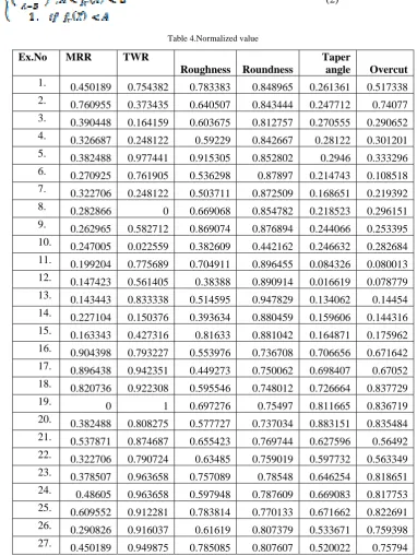
2.4 Desirability functional analysis
Desirability functional analysis is used for optimization of machining parameters. Initially the data are normalized to a common scale [0, 1], combine them using the geometric mean and optimize the overall metric. The normalized data are shown in table 4.The objective of MRR is too maximized; therefore equation (1) is employed for normalization.
For maximization of fr(x), the function is
(1)
Can be used, where A, B and s are chosen by investigator. For the responses like TWR, roughness, roundness, taper angle and overcut, therefore equation (2) is employed for normalization.
(2)
Table 4.Normalized value
Ex.No MRR TWR
Roughness Roundness
Taper
angle Overcut 1. 0.450189 0.754382 0.783383 0.848965 0.261361 0.517338
2. 0.760955 0.373435 0.640507 0.843444 0.247712 0.74077
3. 0.390448 0.164159 0.603675 0.812757 0.270555 0.290652
4. 0.326687 0.248122 0.59229 0.842667 0.28122 0.301201
5. 0.382488 0.977441 0.915305 0.852802 0.2946 0.333296
6. 0.270925 0.761905 0.536298 0.87897 0.214743 0.108518
7. 0.322706 0.248122 0.503711 0.872509 0.168651 0.219392
8. 0.282866 0 0.669068 0.854782 0.218523 0.296151
9. 0.262965 0.582712 0.869074 0.876894 0.244066 0.253395
10. 0.247005 0.022559 0.382609 0.442162 0.246632 0.282684
11. 0.199204 0.775689 0.704911 0.896455 0.084326 0.080013
12. 0.147423 0.561405 0.38388 0.890914 0.016619 0.078779
13. 0.143443 0.833338 0.514595 0.947829 0.134062 0.14454
14. 0.227104 0.150376 0.393634 0.880459 0.159606 0.144316
15. 0.163343 0.427316 0.81633 0.881042 0.164871 0.175962
16. 0.904398 0.793227 0.553976 0.736708 0.706656 0.671642
17. 0.896438 0.942351 0.449273 0.750062 0.698407 0.67052
18. 0.820736 0.922308 0.595546 0.748012 0.726664 0.837729
19. 0 1 0.697276 0.75497 0.811665 0.836719
20. 0.382488 0.808275 0.577727 0.737034 0.883151 0.835484
21. 0.537871 0.874687 0.655423 0.769744 0.627596 0.56492
22. 0.322706 0.790724 0.63485 0.759019 0.597732 0.563349
23. 0.378507 0.963658 0.757089 0.78548 0.646254 0.818651
24. 0.48605 0.963658 0.597948 0.787609 0.669083 0.817753
25. 0.609552 0.912281 0.783814 0.770133 0.671662 0.822691
26. 0.290826 0.916037 0.61619 0.807379 0.533671 0.759398
28. 0.159363 0.540098 0.558079 0.791113 0.569893 0.756705
29. 0.219144 0.883463 0.514171 0.80221 0.577872 0.755359
30. 0.211144 0.984965 0.818103 0.812513 0.596652 0.754573
31. 0.768915 0.824562 0.488583 0.096223 0.464075 0.730558
32. 0.537871 0.880946 0.675149 0.563727 0.450425 0.729884
33. 0.434269 0.839597 0.402194 0.547107 0.494897 0.750982
34. 0.788856 0.827066 0.385858 0.162289 0.494762 0.750084
35. 0.725095 0.182962 0.825526 0 0.517591 0.747503
36. 0.362547 0.843353 0.613365 0.627241 0.36475 0.613511
37. 0.123502 0.972434 0.840936 0.671511 0.356501 0.61194
38. 0.187264 0.946119 0.637258 0.627341 0.377994 0.644933
39. 0.191244 0.956134 0.570022 0.665236 0.391373 0.643362
40. 0.215124 0.209276 0.318276 0.595921 0.427731 0.720907
41. 0.139463 0.708025 0.798942 0.678087 0.301904 0.495118
42. 0.223124 0.984965 0.844114 0.711299 0.299068 0.291774
43. 0.330667 0.984965 0.388761 0.691063 0.338126 0.492874
44. 0.159363 0.983713 0.494735 0.687758 0.342041 0.559084
45. 0.143443 0.666662 0.420429 0.671578 0.343256 0.557962
46. 0.458189 0.843353 0.868078 0.928058 0.436276 0.873639
47. 0.282866 0.10025 0.725201 0.989655 0.046929 0.445629
48. 0.254965 0.498748 0.68837 0.901194 0.414378 0.388284
49. 0.402388 0.269429 0.676985 0.857819 0.218294 0.454607
50. 0.278886 0.966162 1 0.939588 0.587093 0.812928
51. 0.274905 0.804507 0.620993 0.799434 0.551343 0.697228
52. 0.366527 0.457399 0.588406 0.841822 0.7769 0.392773
53. 0.430289 0.414785 0.753763 0.831494 0.411881 0.807317
54. 0.326687 0.582712 0.883065 0.707561 0.240111 0.559084
55. 0.258985 0.248122 0.608697 0.79606 0.737303 0.805072
56. 0.274905 0.791975 0.789605 0.705529 0.347199 0.392773
57. 0.195224 0.868415 0.468575 0.624614 0.252464 0.015486
58. 0.250985 0.582712 0.59929 0.672018 0.333414 0.058018
59. 0.135443 0.498748 0.478328 0.818669 0.468422 0
60. 0.179303 0.395994 0.901025 0.633595 0.726407 0.370329
61. 0.768915 0.914785 0.638671 0.872028 0.611057 0.980361
62. 0.756975 0.931072 0.746057 0.885843 0.583894 0.911794
63. 0.701214 0.961154 0.680241 0.788143 0.751721 1
64. 0.398408 0.914785 0.781971 0.757246 0.82283 0.988217
65. 0.888438 0.848373 0.662422 0.647464 0.803767 0.987095
66. 0.458189 0.843353 0.740118 0.995406 0.307182 0.837616
67. 0.282866 0.10025 0.719544 0.943544 0.824652 0.813601
68. 0.254965 0.498748 0.841784 0.765913 0.489361 0.779598
70. 0.278886 0.966162 0.868509 0.846801 0.663426 0.787566
71. 0.274905 0.804507 0.700885 0.787248 0.769286 0.728426
72. 0.366527 0.457399 0.86978 0.69007 0.336695 0.72764
73. 0.430289 0.414785 0.642774 0.867029 0.674416 0.749074
74. 0.326687 0.582712 0.740259 0.071079 0.344539 0.725396
75. 0.258985 0.248122 0.902797 0.975843 0.451168 0.791606
76. 0.274905 0.791975 0.573278 0.857261 0.151762 0.72764
77. 0.195224 0.868415 0.406361 0.686234 0.243526 0.73774
78. 0.250985 0.582712 0.486888 0.761753 0.252855 0.657951
79. 0.135443 0.498748 0.753339 0.547187 0 0.623162
80. 0.179303 0.395994 0.91022 0.761352 0.159336 0.689373
81. 0.768915 0.914785 0.69806 0.963728 0.314608 0.551229
82. 0.756975 0.931072 0.925631 0.711913 0.329337 0.550107
83. 0.701214 0.961154 0.721953 0.087845 0.867072 0.571429
84. 0.398408 0.914785 0.654717 0.610511 0.414216 0.570306
85. 0.888438 0.848373 0.402971 0.782725 0.128932 0.602963
86. 0.458189 0.843353 0.883637 0.756322 0.195005 0.509707
87. 0.282866 0.10025 0.928809 0.646498 0.480032 0.497363
88. 0.254965 0.498748 0.473455 0.798981 0.350155 0.529907
89. 0.402388 0.269429 0.579429 0.654772 0.200014 0.50634
90. 0.278886 0.966162 0.932411 0.659523 0.519347 0.037818
91. 0.374488 0.843353 0.809755 0.85057 0.584798 0.93985
92. 0.254965 0.708025 0.611734 0.7142 0.82792 0.938727
93. 0.442229 0.248122 0.736092 0.695929 0.818321 0.432162
94. 0.270925 0.289472 0.61018 0.795297 0.534386 0.76804
95. 0.49803 0.768165 0.692113 0.950935 0.568044 0.755695
96. 0.430289 0.830821 0.656694 0.749391 0.590401 0.684884
97. 0.258985 0.414785 0.740047 0.511079 0.449723 0.67254
98. 0.366527 0.164159 0.308727 0.478114 0.598245 0.514084
99. 0.462169 0.248122 0.935737 0.610989 0.584596 0.389406
100. 0.274905 0.021307 0.774477 0.330538 0.516889 0.837616
101. 0.203184 0.843353 0.006639 0.746329 0.025422 0.497251
102. 0.286846 0.692977 0.444181 0.822537 0.196922 0.406352
103. 0.211144 0.874687 0.344429 0.421688 0.476522 0.629896
104. 0.139463 0.582712 0.502016 0.810034 0.341245 0.835596
105. 0.211144 0.805759 0 0.755873 0.433009 0.357985
106. 0.872517 0.908525 0.581054 0.807856 0.359552 0.88935
107. 0.872517 0.733087 0.624814 0.67876 1 0.730894
108. 0.601592 0.248122 0.419723 0.762368 0.92688 0.66244
109. 0.577711 0.921057 0.565996 0.730677 0.724031 0.885984
110. 0.808756 0.927316 0.232946 0.580093 0.996881 0.559084
112. 0.47809 0.978693 0.729093 1 0.732618 0.565818
113. 0.406368 0.979945 0.351498 0.884888 0.49869 0.508585
114. 0.50599 0.971182 0.717637 0.99199 0.633698 0.529907
115. 0.446209 0.269429 0.808766 0.950935 0.651127 0.70845
116. 0.191244 0.804507 0.923223 0.848281 0.246146 0.851195
117. 0.187264 0.979945 0.703992 0.810466 0.323046 0.805072
118. 0.342647 0.665411 0.360341 0.900032 0.470217 0.500729
119. 0.215124 0.822058 0.505195 0.91857 0.24439 0.477163
120. 0.115542 0.540098 0.765289 0.694786 0.534818 0.43104
121. 0.9801 0.982461 0.789965 0.688241 0.340826 0.46841
122. 0.561751 0.832086 0.649208 0.753936 0.443405 0.601728
123. 0.912358 0.580195 0.557938 0.678914 0.34597 0.791606
124. 0.796816 0.74687 0.78904 0.795047 0.398528 0.655706
125. 0.215124 0.531335 0.673736 0.832544 0.505157 0.620918
126. 0.729075 0.540098 0.761334 0.827149 0.099595 0.561329
127. 0.258985 0.941099 0.838316 0.793368 0.469758 0.829873
128. 0.398408 0.895994 0.380843 0.640987 0.515566 0.761306
129. 0.717134 0.913533 0.532061 0.705761 0.108654 0.647851
130. 0.529871 0.912281 0.91022 0.848754 0.457189 0.511952
131. 0.458189 0.874687 0.29367 0.791479 0.231362 0.969251
132. 0.143443 0.982461 0.791307 0.845886 0.151492 0.05813
133. 0.203184 0.966162 0.483703 0.680127 0.478399 0.629896
134. 0.354587 0.968665 0.644398 0.619515 0.207169 0.621928
135. 0.131463 0.972434 0.783595 0.625868 0.394883 0.733139
136. 0.226866 0.848523 0.572141 0.639808 0.113649 0.727528
137. 0.306468 0.457937 0.576315 0.657531 0.240543 0.928628
138. 0.421891 0.986229 0.572 0.650694 0.241771 0.61295
139. 0.421891 0.583125 0.563447 0.663129 0.226758 0.870273
140. 0.199005 0.290185 0.364013 0.651149 0.217173 0.835372
141. 0.470129 0.697997 0.092471 0.55765 0.365695 0.823028
142. 0.334647 0.072684 0.079673 0.544981 0.36691 0.586017
143. 0.290826 0.540098 0.075358 0.521422 0.345146 0.955561
144. 0.254965 0.665411 0.786498 0.525015 0.324747 0.448996
145. 0.438249 0.749374 0.075217 8.79E-05 0.311098 0.953316
146. 0.266945 0.862156 0.753127 0.59725 0.305549 0.34564
147. 0.52191 0.855884 0.704275 0.575697 0.308127 0.827517
148. 0.50201 0.359652 0.728952 0.593149 0.283664 0.916283
149. 0.250985 0.85338 0.752915 0.594673 0.283529 0.825272
150. 0.366527 0.289472 0.781829 0.603763 0.253665 0.82415
151. 1 0.987469 0.462918 0.885444 0.391373 0.994052
152. 0.964139 0.983713 0.436687 0.716277 0.407452 0.484906
154. 0.916338 0.983713 0.462706 0.733915 0.36934 0.999439
155. 0.776915 0.956134 0.426581 0.492969 0.367855 0.638873
156. 0.792836 0.830821 0.49155 0.849523 0.440691 0.502862
157. 0.434269 0.977441 0.491479 0.857046 0.44192 0.771406
158. 0.470129 0.982461 0.5211 0.864317 0.421507 0.905061
159. 0.155383 0.983713 0.545776 0.868433 0.418672 0.701717
160. 0.828697 0.978693 0.520958 0.863122 0.417186 0.62204
161. 0.302806 0.78822 0.546341 0.847485 0.458944 0.68825
162. 0.203184 0.749374 0.546271 0.846981 0.46421 0.574795
163. 0.446209 0.749374 0.5462 0.84261 0.457324 0.955673
164. 0.235065 0.289472 0.545423 0.825823 0.450425 0.842217
165. 0.446209 0.734339 0.545352 0.830754 0.44354 0.784873
166. 0.800796 0.981197 0.138773 0.819841 0.538005 0.705084
167. 0.796816 0.78822 0.090634 0.815303 0.570298 0.917405
168. 0.812736 0.665411 0.425663 0.709409 0.851262 0.343396
169. 0.199204 0.645368 0.21209 0.67103 0.874106 0.12883
170. 0.179303 0.511279 0.212019 0.667328 0.830714 0.127707
171. 0.796816 0.849624 0.344859 0.702296 0.815715 0.238918
172. 0.406368 0.952379 0.344789 0.698009 0.802066 0.372573
173. 0.685254 0.843353 0.158781 0.739268 0.583003 0.394007
174. 0.605572 0.022559 0.138208 0.733999 0.580167 0.437774
175. 0.49803 0.830821 0.15864 0.736839 0.573269 0.48154
176. 0.824716 0.848373 0.077272 0.800047 0.531241 0.817417
177. 0.422328 0.582712 0.019938 0.794108 0.524355 0.917405
178. 0.426308 0.454882 0.019938 0.77586 0.508141 0.468073
179. 0.721114 0.728067 0.206574 0.739385 0.590576 0.35574
180. 0.199204 0.586467 0.206574 0.74783 0.613541 0.479295
2.4.1 Overall desirability (Global desirability)
Overall desirability functional value (D) can be calculated by geometric mean of individual desirability values. If there are “R” number of individual desirability values (d1…… dr) on [0, 1] scale, they can be combined and the
value of D is derived using equation (3). (3) The geometric mean has the property that if any one model is undesirable (dr = 0), the overall desirability is also unacceptable (D = 0).The overall desirability (D) of each experiment is found out and shown in table.5 using weight based approach. MATLAB software is employed to execute the algorithm of PSO for finding the weights of the individual responses.
Table.5Individual and global desirability values
Ex.N MRR TWR Roughness Roundness Taper angle Overcut Global
1. 0.992684 0.903026 0.98505 0.916008 0.988129 0.985346 0.787537
2. 0.99749 0.70014 0.972887 0.912811 0.987657 0.993301 0.608448
3. 0.991385 0.520001 0.969339 0.894864 0.988433 0.972701 0.429938
4. 0.98976 0.603851 0.968201 0.91236 0.988773 0.973479 0.508176
5. 0.991197 0.991776 0.994555 0.918224 0.989182 0.975689 0.86644
6. 0.988057 0.906275 0.962286 0.933214 0.986402 0.95147 0.754705
8. 0.98845 0 0.97551 0.919365 0.986556 0.97311 0
9. 0.987786 0.822465 0.991379 0.932033 0.987527 0.969717 0.718862
10. 0.987218 0.253551 0.942445 0.645806 0.987619 0.972096 0.146263
11. 0.985266 0.912174 0.978656 0.943115 0.97823 0.944998 0.766828
12. 0.982541 0.811452 0.942638 0.939987 0.964192 0.944669 0.643463
13. 0.982294 0.936149 0.959837 0.9717 0.982275 0.957599 0.806738
14. 0.986455 0.503756 0.944098 0.934061 0.983801 0.957566 0.412825
15. 0.983469 0.735137 0.987557 0.934392 0.984085 0.961828 0.631466
16. 0.999076 0.919585 0.964214 0.848979 0.996915 0.991124 0.743099
17. 0.998995 0.978741 0.951831 0.85719 0.99681 0.991087 0.788119
18. 0.998184 0.971155 0.968528 0.855934 0.997162 0.996042 0.798169
19. 0 1 0.977998 0.860191 0.998145 0.996015 0
20. 0.991197 0.925861 0.966715 0.84918 0.998895 0.995982 0.749506
21. 0.994311 0.952701 0.97427 0.869169 0.995862 0.987289 0.78869
22. 0.989649 0.918534 0.972355 0.862659 0.99543 0.987228 0.749322
23. 0.991102 0.986692 0.982977 0.878645 0.996122 0.995528 0.837573
24. 0.993385 0.986692 0.968769 0.87992 0.99643 0.995503 0.828805
25. 0.995456 0.967321 0.985083 0.869404 0.996464 0.995638 0.818183
26. 0.988702 0.96876 0.970567 0.891686 0.994427 0.993854 0.819246
27. 0.992684 0.981561 0.985182 0.891821 0.994197 0.993811 0.845861
28. 0.983246 0.800169 0.964653 0.882015 0.995008 0.993775 0.66192
29. 0.986131 0.956149 0.959788 0.888623 0.995131 0.993735 0.795251
30. 0.985794 0.994532 0.987689 0.89472 0.995414 0.993712 0.856992
31. 0.997585 0.932569 0.95677 0.28526 0.993191 0.992992 0.250413
32. 0.994311 0.955162 0.976054 0.735568 0.992927 0.992972 0.67228
33. 0.992356 0.938688 0.945352 0.723868 0.993759 0.993606 0.629414
34. 0.99782 0.933593 0.942937 0.377462 0.993757 0.993579 0.327378
35. 0.997047 0.540815 0.98824 0 0.994156 0.993502 0
36. 0.990709 0.940205 0.970292 0.778871 0.991064 0.989116 0.690058
37. 0.980942 0.989935 0.989368 0.807858 0.990862 0.989059 0.760639
38. 0.984706 0.980155 0.972582 0.778938 0.991379 0.990223 0.717799
39. 0.984897 0.983897 0.965914 0.803804 0.991686 0.990169 0.738776
40. 0.985963 0.567765 0.931801 0.757785 0.99247 0.992697 0.389433
41. 0.98204 0.882536 0.986246 0.812087 0.989398 0.984377 0.676054
42. 0.986295 0.994532 0.989598 0.833162 0.989314 0.972785 0.778333
43. 0.989871 0.994532 0.943373 0.820377 0.990396 0.984277 0.742712
44. 0.983246 0.994075 0.957509 0.818273 0.990497 0.98706 0.748719
45. 0.982294 0.863518 0.947942 0.807901 0.990529 0.987015 0.635103
46. 0.992845 0.940205 0.991309 0.960786 0.992645 0.996979 0.879873
47. 0.98845 0.435004 0.980371 0.994444 0.973141 0.982058 0.400618
48. 0.987506 0.777433 0.977223 0.945783 0.99219 0.979032 0.689255
50. 0.988321 0.987619 1 0.967163 0.995271 0.995371 0.93522
51. 0.98819 0.924296 0.971032 0.886974 0.994715 0.991954 0.776223
52. 0.990809 0.753461 0.967808 0.91187 0.997756 0.979284 0.643733
53. 0.992272 0.727261 0.98271 0.905859 0.992137 0.995217 0.634302
54. 0.98976 0.822465 0.992357 0.830814 0.987383 0.98706 0.654106
55. 0.987648 0.603851 0.969834 0.884966 0.997291 0.995155 0.508006
56. 0.98819 0.91906 0.985531 0.829534 0.990629 0.979284 0.720292
57. 0.985083 0.950223 0.954305 0.777121 0.987824 0.910867 0.624609
58. 0.987363 0.822465 0.968903 0.808185 0.990272 0.938218 0.590805
59. 0.981775 0.777433 0.955519 0.898345 0.993273 0 0
60. 0.984313 0.71516 0.99359 0.783089 0.997159 0.977994 0.53414
61. 0.997585 0.968281 0.972715 0.929258 0.995626 0.999556 0.868913
62. 0.997442 0.974485 0.982087 0.937117 0.995223 0.997934 0.888441
63. 0.99674 0.985764 0.976507 0.880239 0.997463 1 0.842418
64. 0.991569 0.968281 0.98494 0.861579 0.998266 0.999735 0.813131
65. 0.998912 0.942227 0.974909 0.792227 0.998058 0.999709 0.725313
66. 0.992845 0.940205 0.981603 0.997536 0.98955 0.996039 0.900913
67. 0.98845 0.435004 0.979897 0.969343 0.998286 0.99539 0.405839
68. 0.987506 0.777433 0.98943 0.866849 0.99366 0.994438 0.650649
69. 0.99166 0.622125 0.976719 0.964175 0.998751 0.994716 0.577194
70. 0.988321 0.987619 0.991339 0.914756 0.996355 0.994665 0.877215
71. 0.98819 0.924296 0.97831 0.879704 0.997668 0.992927 0.778696
72. 0.990809 0.753461 0.991429 0.819745 0.990358 0.992903 0.59661
73. 0.992272 0.727261 0.973099 0.926399 0.9965 0.993549 0.644085
74. 0.98976 0.822465 0.981615 0.242529 0.990561 0.992835 0.190595
75. 0.987648 0.603851 0.993711 0.986983 0.992941 0.994779 0.577765
76. 0.98819 0.91906 0.966254 0.920793 0.98336 0.992903 0.788963
77. 0.985083 0.950223 0.945954 0.817301 0.987507 0.99321 0.709793
78. 0.987363 0.822465 0.956565 0.864323 0.987838 0.990667 0.657049
79. 0.981775 0.777433 0.982676 0.723924 0 0.989462 0
80. 0.984313 0.71516 0.994213 0.864079 0.983786 0.991702 0.589999
81. 0.997585 0.968281 0.978066 0.980399 0.989761 0.986747 0.904604
82. 0.997442 0.974485 0.995243 0.833548 0.990164 0.986702 0.787798
83. 0.99674 0.985764 0.980099 0.271671 0.998731 0.987543 0.258032
84. 0.991569 0.968281 0.974205 0.76767 0.992187 0.987499 0.703525
85. 0.998912 0.942227 0.945465 0.876992 0.981934 0.988732 0.757678
86. 0.992845 0.940205 0.992396 0.861016 0.985556 0.985018 0.77433
87. 0.98845 0.435004 0.995454 0.791593 0.99349 0.984477 0.33139
88. 0.987506 0.777433 0.954915 0.886704 0.990704 0.985875 0.63491
89. 0.99166 0.622125 0.96689 0.797005 0.985779 0.984871 0.46157
90. 0.988321 0.987619 0.995691 0.800098 0.994186 0.929267 0.718396
92. 0.987506 0.882536 0.970132 0.834981 0.998321 0.998585 0.703776
93. 0.992522 0.603851 0.981273 0.823467 0.998217 0.981383 0.474426
94. 0.988057 0.638492 0.96998 0.884512 0.994438 0.994106 0.535075
95. 0.993607 0.908962 0.97755 0.973404 0.994979 0.993745 0.849732
96. 0.992272 0.935125 0.974387 0.856779 0.995321 0.991557 0.764507
97. 0.987648 0.727261 0.981597 0.697924 0.992913 0.991153 0.484268
98. 0.990809 0.520001 0.930051 0.673431 0.995438 0.985206 0.316472
99. 0.992924 0.603851 0.99591 0.767992 0.995234 0.979095 0.446861
100. 0.98819 0.248366 0.984355 0.552585 0.994144 0.996039 0.132193
101. 0.985445 0.940205 0.733877 0.854901 0.967846 0.984472 0.553865
102. 0.988577 0.875702 0.951162 0.900618 0.985642 0.98003 0.716341
103. 0.985794 0.952701 0.936352 0.629608 0.993425 0.9897 0.544365
104. 0.98204 0.822465 0.958372 0.893256 0.990477 0.995985 0.682109
105. 0.985794 0.924817 0 0.860742 0.992578 0.977252 0
106. 0.998746 0.965878 0.967057 0.891968 0.990938 0.997377 0.822402
107. 0.998746 0.893717 0.971399 0.812519 1 0.993003 0.699579
108. 0.995336 0.603851 0.947844 0.864696 0.999324 0.990818 0.487753
109. 0.994965 0.970678 0.965492 0.845248 0.99713 0.997292 0.783772
110. 0.998049 0.97306 0.914028 0.746934 0.999972 0.98706 0.654432
111. 0.991927 0.994075 0.984957 0.957103 0.996817 0.990246 0.917558
112. 0.993234 0.992236 0.980694 1 0.997235 0.987325 0.951607
113. 0.99175 0.992695 0.937526 0.936575 0.993827 0.984969 0.846208
114. 0.993752 0.989473 0.979737 0.9957 0.995948 0.985875 0.941844
115. 0.992603 0.622125 0.98699 0.973404 0.996189 0.992309 0.586473
116. 0.984897 0.924296 0.995083 0.915612 0.987601 0.996398 0.816182
117. 0.984706 0.992695 0.978577 0.893512 0.989994 0.995155 0.842056
118. 0.990195 0.862931 0.938965 0.94513 0.993307 0.984626 0.741638
119. 0.985963 0.931544 0.958746 0.955511 0.987538 0.983563 0.817258
120. 0.980341 0.800169 0.983631 0.822742 0.994446 0.981326 0.619511
121. 0.999815 0.993617 0.985559 0.81858 0.990466 0.983155 0.780448
122. 0.994708 0.93564 0.973698 0.859559 0.992788 0.988686 0.764574
123. 0.999157 0.821178 0.964638 0.812618 0.990598 0.994779 0.633791
124. 0.997913 0.899762 0.985487 0.884363 0.991846 0.990591 0.768847
125. 0.985963 0.795446 0.975928 0.906471 0.993941 0.989382 0.682288
126. 0.997097 0.800169 0.983316 0.903319 0.97968 0.987148 0.685363
127. 0.987648 0.97827 0.989178 0.883362 0.993298 0.995832 0.835101
128. 0.991569 0.961035 0.942176 0.78797 0.994121 0.99391 0.699021
129. 0.996946 0.967801 0.961816 0.829681 0.98044 0.990323 0.747581
130. 0.994174 0.967321 0.994213 0.915885 0.993059 0.985115 0.856673
131. 0.992845 0.952701 0.927186 0.882234 0.987057 0.999301 0.76318
132. 0.982294 0.993617 0.985662 0.914226 0.983344 0.938259 0.811465
134. 0.990507 0.988545 0.973251 0.773716 0.986087 0.989418 0.719375
135. 0.981506 0.989935 0.985066 0.777957 0.991765 0.993071 0.733346
136. 0.986445 0.942287 0.966135 0.787193 0.980832 0.9929 0.688455
137. 0.989179 0.753782 0.966569 0.798803 0.987399 0.998343 0.567499
138. 0.992092 0.994994 0.966121 0.794341 0.987444 0.989096 0.73988
139. 0.992092 0.822676 0.965223 0.802439 0.98688 0.996892 0.621918
140. 0.985257 0.639061 0.939552 0.794639 0.986501 0.995979 0.461881
141. 0.99308 0.877992 0.863381 0.731309 0.991087 0.995647 0.543244
142. 0.989979 0.387217 0.855482 0.722359 0.991116 0.988101 0.231991
143. 0.988702 0.800169 0.852548 0.705456 0.990577 0.998982 0.470849
144. 0.987506 0.862931 0.985291 0.708057 0.99004 0.982223 0.578111
145. 0.992439 0.900852 0.852449 0.006712 0.989662 0.99893 0.005057
146. 0.987923 0.947738 0.982659 0.75869 0.989503 0.976484 0.674468
147. 0.994035 0.945237 0.978601 0.743896 0.989577 0.995768 0.674013
148. 0.99368 0.690675 0.980683 0.755895 0.988849 0.998043 0.502099
149. 0.987363 0.944236 0.982642 0.756934 0.988845 0.995707 0.682764
150. 0.990809 0.638492 0.984929 0.763112 0.987866 0.995677 0.467687
151. 1 0.995447 0.95359 0.936891 0.991686 0.999866 0.881829
152. 0.999664 0.994075 0.950164 0.836282 0.992041 0.983918 0.770748
153. 0.998746 0.985299 0.950154 0.830957 0.991463 0.997065 0.768061
154. 0.999197 0.994075 0.953563 0.847253 0.991174 0.999987 0.795384
155. 0.99768 0.983897 0.948792 0.684562 0.991139 0.990014 0.625606
156. 0.997867 0.935125 0.957127 0.91633 0.992734 0.984719 0.800035
157. 0.992356 0.991776 0.957119 0.920669 0.992758 0.994203 0.855991
158. 0.99308 0.993617 0.960581 0.924846 0.992341 0.997768 0.867955
159. 0.983017 0.994075 0.963327 0.927203 0.992281 0.992097 0.859246
160. 0.998273 0.992236 0.960565 0.924161 0.99225 0.989422 0.863259
161. 0.989069 0.91748 0.963389 0.915152 0.993092 0.991666 0.787904
162. 0.985445 0.900852 0.963381 0.91486 0.993193 0.987673 0.767513
163. 0.992603 0.900852 0.963373 0.912328 0.993061 0.998985 0.779668
164. 0.986768 0.638492 0.963289 0.902544 0.992927 0.996161 0.541803
165. 0.992603 0.894269 0.963281 0.905427 0.992791 0.994589 0.764454
166. 0.997958 0.993154 0.885279 0.899035 0.994498 0.992203 0.778377
167. 0.997913 0.91748 0.862313 0.896365 0.995014 0.998071 0.702797
168. 0.998094 0.862931 0.948666 0.831975 0.998568 0.976342 0.662752
169. 0.985266 0.853433 0.908754 0.807548 0.998803 0.955134 0.588683
170. 0.984313 0.784447 0.908735 0.805158 0.998351 0.954947 0.538613
171. 0.997913 0.94273 0.936424 0.827495 0.998189 0.96844 0.704698
172. 0.99175 0.982497 0.936412 0.824785 0.998039 0.978127 0.734655
173. 0.996529 0.940205 0.892667 0.850558 0.995209 0.979353 0.693362
174. 0.995396 0.253551 0.885056 0.847305 0.995166 0.981667 0.184898
176. 0.998229 0.942227 0.853868 0.887338 0.994386 0.995494 0.705439
177. 0.992101 0.822465 0.785398 0.883803 0.994271 0.998071 0.562063
178. 0.992187 0.751958 0.785398 0.872863 0.993993 0.983139 0.499829
179. 0.996997 0.891497 0.907278 0.85063 0.995324 0.977114 0.667121
180. 0.985266 0.82438 0.907278 0.855822 0.995662 0.983661 0.617678
2.5 Fitness function
To find out the weights corresponding to each responses by optimisation algorithms fitness function and constraints are developed, considering the objective of maximizing the overall desirability values and constraint is that sum of the weights should be equal to one,
So the fitness function is, Max f(x) = D1+ D2+ D3+ D4+ ………. + D20
Where D1= d1,1w1 x d1,2w2 x d1,3w3 x d1,4w4 x d1,5w5 x d1,6w6
Subjected to w1 + w2 + ……. + w6 =1
The above equation can be written as
Maximize
20 1 6 1 , ) ( ) ( i j w j i j d x f Subjected to
2.6 Particle Swarm Optimisation (PSO)
The procedure for implementing PSO is given by the following steps
(i) Initialize a population of particles with random positions and velocities in the n-dimensional problem space using a uniform probability distribution function;
(ii) For each particle in swarm, evaluate its fitness value;
(iii) Compare each particle’s fitness evaluation, with the current particle’s Pbest. If current value is better than Pbest, set its Pbest value to the current value and the Pbest location to the current location in n-dimensional space;
(iv) Compare the fitness evaluation with the population’s overall previous best. If current value is better than Gbest, then reset Gbest to the current particle’s array index and value;
(v) Change the velocity and position of the particle using eqn (5) and (6)
(vi) Loop to step (ii) until a stopping criterion is met, usually a maximum number of iterations (generations). (5)
(6)
Where i = 1, 2. . . N is the particle’s index. Variables c1 and c2 are two positive constants, called Cognitive learning rate and Social learning rate, respectively and w is the inertia Weight factor. According to its previous position and its velocity, the variable w is responsible for dynamically adjusting the velocity of the particles. So it is responsible for balancing between local and global search. Hence requiring less iteration for the algorithm to converge. A low value of inertia weight implies a local search, while a high value leads to a global search. Applying a large inertia weight at the start of the algorithm and making it decay to a small value through the PSO execution makes the algorithm search globally at the beginning of the search, and search locally at the end of the execution. In this problem have total six variables, sum of the variables equal to one, constrained particle swarm optimisation is used for solving the problem. Step by step procedure of PSO implementation for this study is described with the help of flow chart in Fig.4
Fig.4.Flow chart
3 Results and discussion
3.1 Particle swarm optimization
0 0.5 1 1.5 2 2.5 3 3.5 4 4.5 5
x 104 102
104 106 108 110 112 114 116 118
Fig.5.Convergence graph
3.2 Ranking
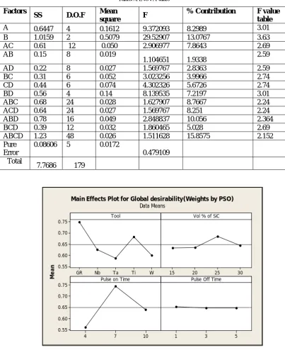
To rank the tools based on the global desirability values, main effect table is constructed by taking average of Global Desirability value corresponding to each tool, pulse on time and off time. Based on Global Desirability value, the tools are rated and the best suited pulse on time and off time is selected, which are shown in the table 6.They ranked the tools as follows; Graphite, Titanium, Niobium, Tungsten, Tantalum. The machinability of workpieces increases when SiC contribution increases till 25% then it start decreasing. Pulse on time of 7 µs and off time of 1 µs is selected as best combination
Table.6.Main effect table
FACTOR/LEVEL 1 2 3 4 5
Max-Min Rank PULSE ON 33.67232 44.6762 38.39074 11.00392 1
PULSE OFF 39.16023 38.77993 38.79914 0.380294 3
workpiece 28.42613 28.5447 30.79568 28.97279 2.369547 2 Tool 26.95299 24.55785 22.5169 21.10954 21.60202
3.3 Analysis of variance
Table.7.ANOVA table
Factors
SS D.O.F Mean
square F
% Contribution F value table
A 0.6447 4 0.1612 9.372093 8.2989 3.01
B 1.0159 2 0.5079 29.52907 13.0767 3.63
AC 0.61 12 0.050 2.906977 7.8643 2.69
AB 0.15 8 0.019
1.104651 1.9338 2.59
AD 0.22 8 0.027 1.569767 2.8363 2.59
BC 0.31 6 0.052 3.023256 3.9966 2.74
CD 0.44 6 0.074 4.302326 5.6726 2.74
BD 0.56 4 0.14 8.139535 7.2197 3.01
ABC 0.68 24 0.028 1.627907 8.7667 2.24
ACD 0.64 24 0.027 1.569767 8.251 2.24
ABD 0.78 16 0.049 2.848837 10.056 2.364
BCD 0.39 12 0.032 1.860465 5.028 2.69
ABCD 1.23 48 0.026 1.511628 15.8575 2.152 Pure
Error
0.08606 5 0.0172
0.479109 Total
7.7686 179
4 Conclusions
EDM of ZrB2-SiC using five different electrodes is carried out at three levels of pulse on and off time. Six responses are considered for optimizing the parameters using desirability functional analysis using PSO. They ranked the tools as follows; Graphite, Titanium, Niobium, Tungsten, Tantalum. The machinability of workpieces increases with Vol % of SiC till it reaches 25% then it starts decreasing. Workpieces with 15 Vol % of SiC shows poor machinability. Pulse on time of 7 µs and off time of 1 µs is selected as best combination.ANOVA shows that tool and pulse on time are the significant factors.
References
[1] Allor R.L. and Jahanmir, S. (1996) `Current problems and future directions for ceramic machining’, American Ceramic Society Bulletein, Vol.75 No.7, pp. 40-43.
[2] Aman Aggarwal, Hari Singh, Pradeep Kumar and Manmohan Singh. (2008) ‘Optimization of multiple quality characteristics for CNC turning under cryogenic cutting environment using desirability function’, journal of materials processing technology, Vol.205, pp.42-50.
[3] Andreas. Nearchou, C. (2011) ‘Maximizing production rate and work load smoothing in assembly lines using particle swarm
W Ti Ta Nb GR 0.75 0.70 0.65 0.60 0.55 30 25 20 15 10 7 4 0.75 0.70 0.65 0.60 0.55 5 3 1 Tool Me a n
Vol % of SiC
Pulse on Time Pulse Off Time
Main Effects Plot for Global desirability(Weights by PSO)
Data Means
[ 4 ] Aysun Sagbas. (2011) ‘Analysis and optimization of surface roughness in the ball burnishing process using response surface methodology and desirability function’, Advances in Engineering Software, Vol.42, pp.992-998.
[5] Chang H.,Lim T.V.(1993)’Evolution of circularity tolerance using Monte Carlo simulation for coordinate measuring machine’,International journal of production research vol.31,pp.2079-2086
[6] Cutler, R. A. (1992) `Engineering property of borides in ceramics and glasses’, In S. J. Schneider (Eds.), Engineered Materials Handbook, ASM International, Materials Park, Vol. 4, pp. 787–803.
[7] Eberhart, R.C. and Kennedy, J. (1995) ‘A new optimizer using particle swarm theory’, proceedings of the sixth International symposium on Micro machine and Human Science, Nagoya, Japan, pp.39-43.
[8] Goldberg, D E. (1990) Genetic algorithms in search, optimization & machine learning, Addison Wesley
[9] Hong Zhang, Heng Li and Tam, C.M. (2006) ‘Particle swarm optimization for resource-constrained project scheduling, International Journal of Project Management’, Vol.24, pp. 83–92.
[10] Indrajit Mukherjee and Pradip Kumar Ray. (2008) ‘Optimal process design of two-stage multiple responses grinding processes using desirability functions and metaheuristic technique’, Applied Software Computing, Vol.8, pp.402–421
[ 1 1 ] In-Jun Jeong and Kwang-Jae Kim. (2009) ‘An interactive desirability function method to multiresponse optimization’, European Journal of Operational Research, Vol.195, pp.412–426
[12] In-Jun Jeong and Kwang-Jae Kim. (2009) ‘An interactive desirability function method to multiresponse optimization’, European Journal of Operational Research, Vol.195, pp.412–426.
[13] Kennedy, J. and Eberhart, R.C. (1995) ‘Particle swarm optimization. Proceedings of IEEE International conference in Neural Networks’. Piscataway, NJ, IEEE service centre. pp. 1942-1948.
[14] Khoshkish, Ashtiani and Goreyshi. ‘Effects of Tool electrode material on electrical discharging machining process of hardened tool AISI D3’, Iran Conference of Manufacturing Engineering
[15] Klocke, F. (1997) `Modern approaches for the production of ceramic components’, Journal of European Ceramic Society, vol.17, pp.457–65.
[16] Mahdavinejad, R.A. (2009) ‘EDM process optimization via predicting a controller model’, International Scientific Journal published quarterly by the Association of Computational Materials Science and Surface Engineering, Vol.1 No.3, pp.161-167
[17] McGeough, J.A. (1988) Advanced methods of machining, Chapman & Hall, New York.
[18] Monteverde, F., Bellosi, A.and Luigi Scatteia. (2008) `Processing and properties of ultra-high temperature ceramics for space applications’, Materials Science and Engineering, vol. 485, pp. 415–21.
[19] Mu-Chen,C.Du-Ming, T. Hsien-Yu,T.(1999)’A stochastic optimization approach for roundness measurements’,Pattern Recognition Letters,Vol,pp.707–719
[20] Ritchie Mae gamut and armacheska mesa. (2008) ‘Particle Swarm Optimization - Tabu Search Approach to Constrained Engineering Optimization Problem’s’, World Scientific and Engineering Academy and Society transactions on mathematics, Vol. 7 No.11,pp.666-675.
[21] Schwartz, M.M. (1995) Engineering applications of ceramic materials, American Society of Metals, Metals Park, Ohio.
[22] Surajit Pal and Susanta Kumar Gauri. (2010) ‘Assessing effectiveness of the various performance metrics for multi-response optimization using multiple regression’, Computers & Industrial Engineering, Vol.59 pp. 976–85.
[23] Thakshila Wimalajeewa and Sudharman K. Jayaweera. (2007) ‘PSO for constrained optimization optimal power scheduling for correlated data fusion in wireless sensor networks’, the 18th Annual IEEE International Symposium on Personal, Indoor and Mobile Radio Communications (PIMRC’07).
[24] Upadhya, K. Yang, J M and Hoffman, W. P. (1997) `Materials for ultrahigh temperature structural applications’. American Ceramic Society Bulletin, vol.76 No.12, pp.51–56.