On th e ex isten ce and uniqueness o f estim a tes in
robust and heteroscedastic regression m odels
Thesis subm itted to the University of London for the degree
of Doctor of Philosophy in the Faculty of Science
b y
Adam Crisp
University College London
P r o Q u e s t Number: 1 0 0 1 6 7 2 5
All rights re s e r v e d
INFORMATION TO ALL U S E R S
T h e quality of this reproduction is d e p e n d e n t upon the quality of the c o p y subm itted. In th e unlikely e v e n t that the author did not s e n d a c o m p le t e manuscript
and there are m issin g p a g e s , t h e s e will b e noted. A lso, if material had to be rem o v ed , a note will indicate th e deletion.
uest.
P r o Q u e s t 1 0 0 1 6 7 2 5
P u blish ed by P r o Q u e s t LLC(2016). Copyright o f the D issertation is held by th e Author. All rights re s e r v e d .
This work is protected a g a in s t unauthorized cop ying under Title 17, United S t a t e s C o d e . Microform Edition © P r o Q u e s t LLC.
P r o Q u e s t LLC
7 8 9 E a st E is e n h o w e r Parkway P.O. Box 13 4 6
A b stra ct
The thesis studies redescending M -estim ators for the ordinary linear regression
model, and m axim um likelihood estim ators for heteroscedastic regression models.
In general, redescending M -estim ators do not yield unique estim ates of the model
param eters, and the thesis shows th a t the difficulties associated with this have
not always been fully appreciated in the literature. This motivates the develop
m ent of an approach whereby unique redescending M -estim ates can be reliably
obtained. This is achieved by embedding the linear model within a m ultivari
ate t location-scatter framework, which is known in the literature for its desirable
uniqueness properties. M -estim ates derived from the conditional t distribution are
also considered, but it is shown th at the resulting objective function is intrinsically
m ultim odal, with modes of infinity.
The nonregularity result for the conditional t model is found to have impli
cations for heteroscedastic regression models. Two classes of commonly proposed
models are considered. The first is found to yield an unbounded likelihood at
points corresponding to nonreplicated observations, whilst for the second a much
stronger linear independence condition is obtained for the likelihood to be un
bounded.
The thesis concludes with a discussion of efficient methods for testing analytical
conditions arising from the preceding studies.
Keywords: conditional distribution, heteroscedastic regression, mean-variance re
lationship, multimodality, m ultivariate t distribution, redescending M -estim ator,
A ck n ow led gem en ts
I would like to thank my supervisor, Jim Burridge, for the ideas, encouragement
and friendship th a t he has offered over the last few years. Thanks are also due to
the many people who have given me support and advice. I would like to mention
in particular M aria Efstathiou, Costas Goutis, Kostas Skouras, Steve G alii van and
an Associate Editor of Biometrika. I also thank Charles Hayward, who got me
C on ten ts
In tro d u ctio n 6
1 A f-estim a to r s 9
1 .1 In tro d u c tio n ... 9
1.1 .1 Simple Location M o d e l... 9
1.1.2 Linear Regression M o d e l... 12
1 . 2 Redescending M - e s tim a to r s ...13
1.2.1 General R e m a r k s ... 13
1.2.2 The Uniqueness P ro b le m ... 17
2 On th e uniq u en ess o f M -estim a tes 19 2 . 1 In tro d u c tio n ...19
2.2 E x a m p l e s ...20
2.3 Analytical C o nditions... 24
2.4 D iscu ssio n ...26
3 U n iq u e R ed escen d in g M -e stim a te s for th e linear m o d el 28 3.1 In tro d u c tio n ...28
3.2 M ultivariate t M e th o d o lo g y ... 30
3.2.1 Location-Scatter M odel... 30
3.2.2 Linear Regression M o d e l... 32
3.3 E x a m p l e s ...34
3.4.1 Main R e s u l t ... 43
3.4.2 Additional Remarks ... 45
3.4.3 Alternative A pproaches... 51
3.5 D iscu ssio n ... 54
4 N on regu lar L ik elih ood s in H etero sced a stic R egression 56 4.1 In tro d u c tio n ... 4.1.1 General R e m a r k s ... 4.1.2 Heteroscedastic Regression Models 4.2 Main R e s u l t s ... 4.2.1 Model 1 ... 4.2.2 Model 2 ... 4.3 E x a m p l e s ... 4.4 D iscu ssio n ... 56 56 57 58 58 59 61 66 5 T estin g th e e x iste n c e o f m axim u m lik elih ood e stim a te s 68 5.1 In tro d u c tio n ...6 8 5.2 Description of a lg o rith m s... 70
5.2.1 Parallel H y p e rp la n e s ... 70
5.2.2 Condition D * ...73
5.3 E x a m p l e s ... 74
5.4 D iscu ssio n ... 76
6 C on clu d in g R em arks 77 A L ik elih ood F ittin g 80 A .l Full Multivariate t M -e s tim a te s ... 80
A.2 Conditional ^ M -e s tim a te s ... 82
A.3 Calculation of D e r iv a tiv e s ...84
In trod u ction
The work reported here relates to the study of redescending M -estim ators for
the ordinary linear regression model and maximum likelihood estim ators for het-
eroscedaatic regression models. The connection between these topics arises from
the development of an approach th at overcomes the well-known uniqueness prob
lems associated with redescending M -estimators.
An M -estim ator is one of many estim ators th at define statistics which are
in some sense robust (Hampel, Ronchetti, Rousseeuw, and Stahel, 1986). Such
estim ators arise from the need to construct procedures which are not too sensitive
to deviations from assumptions, such as normality and independence, th a t form
the foundations upon which many classical procedures are built. For example,
a common type of deviation is the presence of outliers, namely d ata which are
away from the p attern set by the majority. These may be due to a genuinely
long-tailed distribution or perhaps mistakes made in data collection and can, for
example, have an arbitrarily large effect on estim ates obtained from methods of
least-squares.
Robust methods probably date back to the prehistory of statistics (Hampel
et al., p. 34), although a general theory regarding robust estim ation has really
only evolved over the last thirty years or so. A key development in this area
was the introduction of the M -estim ator (Huber, 1964) for robust estim ation of a
location param eter, and generalisations to more complicated estim ation problems
which are attractive in term s of their robustness properties b ut do not usually
guarantee unique estim ates of the model param eters. This has led to research
into obtaining sufficient conditions under which a given sample will yield a unique
redescending estim ate, b ut these are not always useful. It is therefore of interest
to consider an approach whereby unique redescending M -estim ates can be reliably
obtained, and this provides the principal motivation for the work presented here,
which is structured as follows.
Chapter 1 presents an introduction to M -estim ators and reviews the case for us
ing the sub-class known as redescenders. This discussion is continued in C hapter 2
where attention is brought to an im portant, but generally unrecognised difficulty
th a t can arise within the redescending framework. This is found to affect strongly
the uniqueness results for the linear model obtained by Rivest (1989), and provides
further motivation for the development of a new redescending approach.
Such an approach is considered in Chapter 3, where it is proposed th a t unique
redescending estim ates may be obtained if the linear model is embedded within
a m ultivariate location-scatter model. Sufficient conditions for the existence of
unique estim ates in the location-scatter caise have been developed by Kent and
Tyler (1991), and these are of particular use when applied to the m ultivariate t
distribution. Unique estimates for the linear model param eters are obtained from
unique redescending estimates of location and scatter, and examples based on real
d ata sets presented. They suggest th at the m ultivariate t approach is a useful
addition to the methods for robust regression already available. M -estim ates
derived from the conditional t distribution are also considered, but it is shown
th a t the resulting objective function is intrinsically m ultimodal, with modes of
infinity.
In Chapter 4 the nonregularity result for the conditional t model is found to
have wider implications. It is observed th at the essence of the problem lies in the
heteroscedastic form of the conditional t model, and this motivates a more gen
proposed models are considered. The first is found to yield an unbounded likeli
hood at points corresponding to nonreplicated observations, whilst for the second
a much stronger linear independence condition is obtained for the likelihood to be
unbounded. Numerical examples explore the practical difficulties th at can arise
in these cases.
Chapter 5 discusses efficient methods for testing two existence conditions aris
ing from the m ultivariate t and heteroscedastic regression studies, and concluding
remarks are presented in Chapter 6. Some com putational details are included in
C hapter 1
M
-estim ators
This chapter presents background m aterial in order to ‘set the scene’ for following
chapters. It is divided into two sections. The first provides an introduction to
M -estim ators and how they are defined for the linear model. The second section
deals with the sub-class known as redescending M -estimators.
1.1
Introduction
1.1.1
Sim ple L ocation M od el
The definition of an M -estim ator may be motivated by considering the m ethod of
maxim um likelihood estim ation for a one-dimensional location param eter. Sup
pose X i , . . . are independent and identically distributed (i.i.d.) one-dimensio
nal random variables. A param etric model may be defined as a family of probabil
ity distributions Fq on the sample space, indexed by an unknown location param e ter 6 belonging to some param eter space 0 . Denoting the densities as fe the well-
known maximum likelihood estim ator is defined as the value T„ = Tn(ATi,. . . ,X „)
which maximises H* or equivalently by the value T„ which minimises
may achieve more robustness, and so considered estim ators th a t can be defined
by a more general minimization principle of the form:
Tn minimises (1.1) 1=1
where p is a non-constant function. If p has a derivative xj)(x^O) = (dldO)p(x^O)^
then for useful choices of p the estim ator satisfies the implicit equation
è v - ( ^ ; ,r n ) = 0. (1.2)
*=1
D e fin itio n 1.1. Any estim ator defined by (1.1) or (1.2) is an M -estim ator.
Though (1.1) and (1.2) are not always equivalent, for the sake of brevity M-
estim ators are often defined through a given ^-function. For example, ÿ = —f ' / f
is equivalent to maximum likelihood estimation. Typically ^ is odd and, if strictly
monotonically increasing, will yield a unique solution to (1.2) due to the convexity
of p. Otherwise a solution to (1.2) may not be unique and difficulties may arise.
These are discussed in Section 1.2 and in Chapter 2. There follow some examples
of monotone ■0-functions.
E x a m p le 1.1. The Huber M -estim ator (Huber, 1964) with cut-off point c is given
by
0 c(z) = m in{c,m ax{x, —c}}
for 0 < c < G O. It has minimax variance over the distributions contained in
a particular neighbourhood of the normal distribution (Hampel et al., 1986, p.
172).
E x a m p le 1.2. A similar, and perhaps aesthetically more pleasing example arises
from the distribution function of the scaled logistic distribution F(j(x) = { 1 -f
exp(—a:/<j)}"^, for which we obtain the strictly monotone
where 0 < a < oo. The scale param eter a is equivalent to the Huber cut-otF
point c in th a t the larger c and cr are, the more similar the solution will be to
least-squares, whilst smaller values tend to give more robustness.
Robustness properties of an estim ator may be obtained via th e influence fu nc
tion (Hampel et al., 1986, p. 84). It describes, at some underlying model distri
bution F , the effect of an infinitesimal contamination at a point on an estim ator,
standardised by the mass of the contamination. For M -estim ators it reduces to
(Hampel et al., 1986, p. 103), under the assumption th at the denominator is
nonzero. Among the measures th a t can be derived from the IF are the following
(Hampel et al., 1986, pp. 85-88): the asym ptotic variance of the estim ator, which
is simply the expected square of the IF; the gross-error sensitivity of ÿ at given
by
7* = s u p |I F ( a ;;ÿ ,F ) |;
X
and the rejection point
p* = inf{r > 0; lF{x;xj^,F) = 0 when |ar| > r}. (1.3)
(If there exists no such r, then p* = oo.) Thus all observations further away
than p* are rejected completely. The Huber and logistic M -estim ators both have
p* = oo. M -estim ators for which p* is finite will be discussed in Section 1.2.
The gross-error sensitivity measures the worst influence which a small am ount
of contam ination of fixed size can have on the value of the estim ator, and so it
is extremely desirable th at 7* be finite. In such cases ÿ is described as B-robust
at F. It can be shown th at, if F has a unimodal and symm etric density / th a t
satisfies certain differentiability conditions (Hampel et al., 1986, p. 125), then ÿ
is B-robust if and only if |ÿ | is bounded (Hampel et al., 1986, p. 132). It follows
Furthermore, for a given upper bound on 7*, the Huber ^ is optim al (in term s
of asym ptotic variance) B-robust at F = Clearly an estim ator cannot be B-
robust if ÿ) is unbounded: for example, the sample mean is not B-robust, since it
corresponds to ^p(x) = x.
1.1.2
Linear R egression M od el
We now move on to consider the linear regression model, which contains the loca
tion model as a special case:
î/i = xfp-f-e.-, (1.4)
where {(j/i,x,): i = 1, . . . , n} is a m ultivariate sample of size n for y* € R and
X,- G R^, 3 is a vector of unknown param eters belonging to R^ and the {e,} are i.i.d. with distribution function F(e*/cr), where <j > 0 is an unknown scale
param eter. The form of (1.2) can be easily extended to cope with this more
complicated estim ation problem. A more general form of (1.1) defines the M
-estim ator for 3 (Huber, 1973; Hampel et al., 1986, p. 311) as the value 3 th at
minimises
or, on taking derivatives, solves the vector equation
(1.6)
where again, ÿ = p'. Thus p[i) = defines the least-squares estim ator. There
remains the question of estim ating cr. A natural approach is to consider an
M-estim ator for cr, which may be defined as the solution of
where % is some given function. For example, if we take %(t) = sgn(| 11 — 0.6745),
(Hampel et al., 1986, p. 107), we obtain
which is a robust estim ator for scale. The division by % 0.6745 ensures
Fisher-consistency (Hampel et al., 1986, p. 83) when the d ata are normally dis
tributed. Estim ates ^ and d of P and cr m ay then be calculated by solving the
system of equations (1.6) and (1.7). Algorithms for this task are considered by
Huber (1981, Chapter 7).
Unfortunately, the M -estim ator defined by (1.6) can only have bounded in
fluence with respect to outliers in the response variable (Hampel et al., 1986, p.
313). Robustness against outliers in the x space may be obtained via a generalised
M -estim ator for defined as a solution to
è {Vi - x f P)/(T}x, = 0 (1.9)
t =l
(Hampel et al., 1986, p. 315), where the function 77 may be w ritten in the form
?7(x,]() = w{x) • -0 (f • u(x)).
The Huber M -estim ator thus corresponds to w{x) = v{x) = 1. Robustness against
outliers in the x space is achieved through the weight function w, which involves
a robust covariance m atrix in the x space, to be determined by the solution of
further implicit equations. For details, see Hampel et al. (1986, pp. 315-328).
1.2
R edescending iVf-estim ators
1.2.1 G eneral R em arks
We return now to the Huber M -estim ator (1.6). In the preceding section it was
from non-unique solutions. This is im portant since non-monotone ^-functions are
of great interest. The main examples of such functions are the so-called redescen
ders, and these are considered in the present section.
The motivation for redescending M -estim ators arises from the rejection point
p* (1.3). Hampel et al. (1986, p. 8 8) say th a t it is desirable for p* to be finite,
th a t is to say for M -estim ators th at there exists a fixed constant 0 < r < oo such
th a t ÿ (f) = 0 for all | f | > r. M -estimators with such ÿ-functions are described by
Hampel as being redescending. However, this definition has not always been used
in the literature: for example, Maronna and Yohai (1981) and Novovicova (1990)
use the term to describe functions such th at ÿ(f) 0 as 111 — oo, and Holland
and Welsch (1977) use the terminology “soft redescender” to describe ^-functions
th a t merely tend to zero, and “hard redescender” when Hampel’s condition is sat
isfied. Indeed, “soft” redescenders, such as th a t used in the maximum likelihood
estim ator for the Cauchy distribution, give very little influence to extrem e obser
vations and behave almost like estimators with low rejection point, even though
their rejection point is infinite (Hampel, 1974). Following Kent and Tyler (1991)
who use the term “strong redescender” for ^-functions th a t vanish outside some
central region, we shall observe the following:
D e fin itio n 1.2. If xp(t) ^ 0 as | —»• oo, ÿ is weakly redescending. If ÿ(^) = 0
for 111 > r, where 0 < r < oo, ^ is strongly redescending.
It should be noted th at the distinction between the two is im portant, as some
conditions related to the existence and uniqueness of redescending M -estim ators
do not apply in both cases (Kent and Tyler, 1991). Here then, are some examples
of redescending "^-functions, illustrated graphically in Figures 1.1, 1.2 and 1.3:
function^ advocated by Andrews (Andrews et al., 1972):
V’s i n ( a ) ( 0 —
sin (t/a) if I i I < ott,
0 otherwise.
E x a m p le 1.4. In Andrews et al. (1972) Hampel proposed a three-part (strongly)
redescending M -estimator:
^a,6,r( 0 — t
asgn{t) ( r - \ t
- b
0
if 0 < 1^1 < a,
i î a < \ t \ < b ,
sgn(t) if 6 < 111 < r,
otherwise,
where 0 < a < b < r < oo.
E x a m p le 1.5. A weakly redescending M -estim ator is obtained from the p-dimen-
sional t distribution on i/ > 0 degrees of freedom:
{u + p) t
W t e
All redescending M -estimators are B-robust since |ÿ | is bounded by definition
(Hampel et al., 1986, p. 153). However, it is their ability to reject extreme out
liers which makes them preferable to monotone ^-functions. Hampel et al. (1986,
pp. 166-167) compare the asymptotic variances for some strongly redescending
location M -estim ators with those of the Huber and scaled logistic M -estimators.
They find th a t the Huber and logistic are the most efficient at the normal model
and th a t they do well at relatively short-tailed distributions. However, their vari
ance goes up considerably at distributions which produce large outliers, where the
redescenders are up to 20% more efficient. At such distributions, the monotone ÿ
an —ani
Figure 1.1: Andrews’ sine function.
-b —r - a
Figure 1.2: Shape of Hampel’s three-part redescending ÿ»-function.
1.2.2
T h e U niqueness P roblem
Though the motivation for using redescending M -estim ators is clear, their lack of
monotonicity ensures th a t if a solution to (1.6) exists, it may not be unique. To
counter this difficulty, several approaches have been proposed. Klein and Yohai
(1981), in a study of asymptotic behaviour, overcome the difficulty by defining
the estim ate as the limit (if it exists) of a given iterative sequence, and Huber
(1981, p. 192) suggests th at one might ‘start with a monotone ÿ , iterate to death,
and then append a few ( 1 or 2) iterations with the non-monotone However,
Huber does not discuss the choice of monotone ^ or the adequacy of the solution
thus obtained. This is perhaps not too surprising, given his earlier comments (p.
103) to the effect th at, in his opinion, the difficulties associated with redescenders
more than offset the improvements in asymptotic variance obtained at heavy-tailed
distributions.
A similar approach is to compute only a one-step M -estim ator (Bickel, 1975),
where the estim ate is computed from one iteration of a Newton-Raphson type
algorithm, using a robust estim ate for the starting value. For non-monotone ÿ
the estim ator is safe in th at the problem of uniqueness is avoided, but the approach
is somewhat circular in th at one requires a robust estim ate in order to obtain a
robust estimate.
For the regression problem, a very robust starting value for P is the least median
o f squares estim ator (Rousseeuw, 1984), defined as the value th a t minimises
m s = M E D { ( ÿ i - x f p f }
over P, but this proposal presents great com putational difficulties, though algo
rithm s are available (Souvaine and Steele, 1987).
R ather than develop alternative computational strategies, one might consider
obtaining sufficient conditions for a system of estim ating equations to yield a
unique solution. This can be done even if one specifies only th a t the equations are
is th a t the conditions obtained are extremely strong, and almost impossible to
test for all but the simplest of problems. Conditions have been developed for
the Af-estimation framework by, for example. Maronna and Yohai (1981) and
Rivest (1989). However, these do not seem to provide a straightforward means
of testing the uniqueness (or indeed existence) of a solution to (1.6). Indeed,
the results in Rivest (1989) warrant detailed consideration, for in the event th at
(1.6) does not adm it a unique solution, Rivest defines P as the value of P th at
corresponds to the global minimum of (1.5). The tacit assumption is th a t the
global minimum is attained at a unique value of p. However, this need not be the
C hapter 2
On th e uniqueness o f M ’-estim a tes
2.1
Introduction
Rivest (1989) considers the uniqueness of M -estim ators for the linear model (1.4).
The M -estim ator of (3 is defined as the solution of
where c is a ‘positive constant of robustness’, and a is to be estim ated by (1.8). It
is noted th at (1.8) is a special case of a generalised estim ator for <7, given by the
solution to
(2.2)
where %(f) is an even function, increasing in [0, oo), and 7 = E [%(%)], where Z
is a A/’(0 ,1) random variable. One of Rivest’s objectives is to obtain sufficient
conditions concerning ^ and % so th at the non-linear system (2.1) and (2.2) has
a unique solution; however, they do not seem to be complete. Defining ÿt(^) =
0 (</Â;), the non-linear system
è - x f P ) = 0 (2.3)
is considered. For monotonie ip, the system adm its a unique solution P*; in the
contrary caae, Rivest defines P t as the solution of (2.3) which minimises
For a given P;t, Rivest also defines
Rivest claims th at for strongly redescending tp the definition of p t excludes from
the study all the solutions of (2.1) and (2.2) which do not minimise (2.4). However,
the possibility th at (2.4) does not uniquely define Pit has not been acknowledged.
To examine the uniqueness of the solution to (2.1) and (2.2), Rivest states th at
an equivalent problem is to find a value of k for which k = and proceeds to
consider k /c k as a function of k. If k/(Tk is increasing, he writes, the system has
a unique solution for all c. By way of example, for various ÿ and sets of data
Rivest evaluates the function k/(Tk at 60 equidistant values of k^ and the points
{kjk/(7k) thus obtained are joined to form a continuous curve. By joining the
points Rivest implicitly assumes continuity, but this need not be the case. For
example, if at some k the global minimum of (2.4) is attained at more than one
value of p, then Pit will not be uniquely defined. This means th at CTk will not be
uniquely defined either, and so the function k/a k need not be continuous at values
of k corresponding to a switch from one solution to another. Examples of this
behaviour are given in the next section, and these are followed by discussion of
the implications for Rivest’s analytical conditions.
2.2
E xam ples
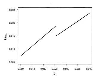
E x a m p le 2.1. Consider the univariate case = x ^P , where fi is the location
param eter of a Cauchy density with scale param eter a:
a
0.025
0.020
-^ 0.015
-0.010
-0.005
0.030 0.035 0.040
0.010 0.015 0.020 0.025
Figure 2.1: Discontinuity from use of Cauchy Af-estimator on clustered data.
Take ÿ = —f ' / f as a weakly redescending function, and without loss of generality
take c = 1. The estim ator fik is thus defined as the solution of
E
= 0. (2.6)■tï + iVi
-For the highly clustered data set
y = (-1 .0 3 , -1 .0 2 , -1 .0 1 , -1 .0 0 , -0 .2 , -0.1,0.95,1.0,1.05,1.10,1.12),
solutions to (2.6) satisfying (2.4) were found for 100 equidistant values of k in
the range (0.01,0.04), and the points {k, k/ ak) thus obtained are presented in
Figure 2.1.
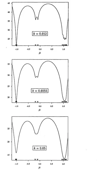
The discontinuity present at A: % 0.0255 is caused by a switch in the estim ate
of the location param eter /z from the cluster around -1 to th at around -f-1. This
can be seen in the plots of p{{yi ~ p ) / ^ } against /z (i.e. minus the log-likelihood
against /z) presented in Figure 2.2. For large k the function becomes unimodal,
and non-uniqueness is no longer a problem, but for k 0.0255 there exist two
40
-k = 0 .0 1 2
-0.5 0.5
-1.0 0.0 1.0
/i
35
30
25
k = 0.0255
20
X X
-1.0 -0.5 0.0 0.5 1.0
25
20
k = 0.05
15
-0.5
-1.0 0.0 0.5 1.0
noted th a t in the narrow range of values for k considered here, the slow change in
the estimates /zjt either side of the discontinuity gives rise to a near constant cTk]
hence the linearity present in Figure 2.1).
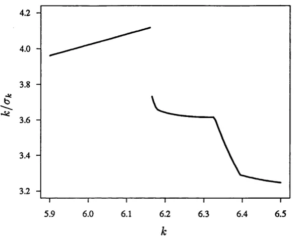
E x a m p le 2.2. Rivest gives an example based on the “Stack-Loss” data (Brown
lee, 1965), comprising 21 observations on y = stack-loss and three covariates.
Using the strong redescender 0 = V>sin(o), with a = 1/tt, Rivest obtains a continu
ous graph of the function k/ak. However, it includes a suspiciously steep drop in
the region of A: = 6.2. When examined in detail, this is found to be a discontinuity
caused by the same problem outlined in Example 2.1. For instance, at A; = 6.164,
both
0.808 0.548 \ -0 .0 7 0 y
and =
^-39.098^ 0.890 10.537 -0 .0 9 4 y
are solutions to (2.3), with minimising (2.4). This yields ak = 1.4966. How
ever, aX k = 6.1645, is the solution th at minimises (2.4), giving ak = 1.6503.
There exists a A;* % 6.16435 for which the solutions give the same value of (2.4),
and so ak* is not uniquely defined. The function k/ak is therefore not continuous,
as shown in the magnified section of Rivest's graph given in Figure 2.3.
The question arises as to which of the estimates for pjt* one should take. An
additional criterion may be to choose the one with minimal residual sum of squares.
However, when other values of k are considered, this is not necessarily consistent
with (2.4). For example, p6!i64 above minimises (2.4) but has a smaller
residual sum of squares. In any case, Rivest's method for examining the function
k/a k is clearly inadequate, and in the light of this result, other examples presented
4.2
-b
3.2
6.5
5.9 6.0 6.1 6.2 6.3 6.4
Figure 2.3: Discontinuity from use of sine M -estim ator on Stack-Loss data.
2.3
A nalytical C onditions
The implications of the previous discussion for Rivest’s analytical conditions are
now considered. Further to the generalised estim ator for the scale param eter
defined by (2.2), let ak be the solution to
Rivest argues th at the non-linear system (2.1) and (2.2) has a unique solution for
a given value of c if
(2.7)
has a unique solution, and th at therefore, in considering without loss of generality
the case c = 1, this is equivalent to ^ x t ( y * — x ^ P t) being a decreasing function
of k, where Xk{t) = x(V^)* Following the results of Section 2.2, this argument
is flawed, for values of k may exist where P t minimising (2.4) is not unique.
Therefore, '^XkiVi — xf P^) may be decreasing, but due to a discontinuity there
0.8
b
0.4
-0.2
0.0 0.5 1.0 1.5 2.0
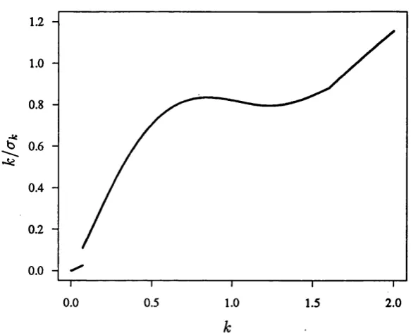
Figure 2.4: Second Cauchy M -estim ator example. Note th at k/ak increases mono- tonically for Â; > 2.
example, returning to the Cauchy M-estimator of Section 2 .2 , if the d ata set is changed to
y = ( - 1 . 1 , - 1 . 0 5 , - 1 . 0 3 , - 1 . 0 , - 0 . 9 7 , - 0 . 9 5 , 0 . 9 7 , 1 . 0 3 , 1 . 0 5 , 1 . 1 , 1 . 2 , 1 . 3 5 , 1 . 5 ) ,
the k/cTk function given in Figure 2 .4 is obtained, where 2 0 ,0 0 0 equidistant values
of k are taken in the range ( 0 . 0 0 0 1 ,2 . 0 ) . Here, at A: % 0 .0 7 1 4 , the discontinuity jum ps in the opposite direction to th at shown in Figure 2 .1 , and since —»■ 0
85 A; 0, it seems th at there exist values of c for which = c has no solution.
Therefore, Rivest’s argument would be more accurately expressed by saying that
if the function kja ^ is increasing, then the system has at most a unique solution
for all c.
Turning now to the analytical conditions, whilst assuming th a t ^ and % are
-1
T r i - x /
»=1 .3=1 i= i
function X) Xk{yi — x f pjt) is decreasing for a given value of k if and only if
x K n ) > 0 (2.8)
where r,- = y,- — '4>'k[y) = i^'{ylk) and Xk{y) ~ x \ y ! ^ ) for values of k for
which is an invertible m atrix. Furthermore, in th e case where the
scale param eter is defined by (1.8), Rivest proposes th at the system (2.1) and (1.8)
has a unique solution if, for all k and for all z = 1, . . . , n,
- 1
0.6745 > SixJ
i=i 3=1
(2.9)
provided th at ^DxjxJV’U^i) is invertible, where s,- = sgn(r,).
Two points arise here. Firstly, it has already been shown th a t ÿ and % cannot
be assumed to be continuously differentiable, and so the validity of (2.8) and
(2.9) as conditions for uniqueness requires clarification. For example, (2.9) may
be satisfied for all k where is defined, but the behaviour of the function k/(7k
at discontinuities and its effect on the existence of solutions to (2.1) and (1.8)
remains unclear. Secondly, even if some proposed condition for the existence of
for all k is satisfied, it is not immediately obvious how the conditions (2.8) and
(2.9) may be put to profitable use, for to test (2.9) one is apparently faced with
the task of finding |3jt for aU & — a non-trivial problem in all but the simplest
cases.
2.4
D iscussion
A ttention has been drawn to a problem th at all too easily may be overlooked.
T hat the system of equations (2.3) may not have a unique solution has been
appreciated by Rivest, but he has not considered the possibility th at the solution
corresponding to the global minimum of (2.4) may also be non-unique. In this he
redescending M-estimates for the univariate case, both Huber (1981, p. 54) and
Hampel et al. (1986, p. 152) state th at one way of overcoming the problem is to
take the global minimum. This is curious, since when discussing the linear model,
Hampel et al. (1986, p. 339) note th at there may be m ultiple global solutions to
the minimization problem.
In considering solutions to (2.3), it has been demonstrated, in examples using
both artificial and real data, th at even the “optim al” estim ate of the regression
param eter Pt, in the sense of minimising (2.4), is not necessarily unique. This
suggests th at, if redescending ^-functions are to be used, then the estim ator for
P should be defined in a different way. An alternative definition is considered in
C hapter 3
U niq u e R ed escen d in g
iU -e stim a tes for th e linear m od el
3.1
Introduction
In the previous chapter we saw the complications th a t can arise when using re
descending M -estim ators for the linear model. In this chapter, a redescending
approach is developed th at does not suffer these drawbacks, since unique esti
m ates will, in general, be obtained. This is achieved by application of recently
developed results for the existence of unique weakly redescending M -estimates
for the location-scatter model, and in particular, for location-scatter estimates
corresponding to the multivariate t distribution.
A p-dimensional t distribution on i/ > 0 degrees of freedom gives rise to a
weakly redescending ^-function:
(3 1)
This ^ is appealing in th at the degrees of freedom param eter i/ may be regarded
down-weighting on outliers increases with decreasing i/, and since in the lim it as i/ —+ oo,
—*■ t, (3.1) includes least-squares as a special case.
The t distribution has been widely considered as an alternative to the strict as
sum ption of normality th at is often made in classical statistical inference. M aronna
(1976) presents an example using t M -estimates for m ultivariate location and scat
ter, and Pendergast and Broffitt (1985) mention the t distribution as a potential
M -estim ator for growth-curve models. Zellner (1976) considered inference un
der an assumed m ultivariate t distribution on the vector of errors in the linear
regression model, and Sutradhar and Ali (1986) generalised this to m ultivariate
regression. However, the models contained therein are of no use in the context
of robust regression, since the resulting objective function is maximised at the
least-squares estim ate.
Lange, Little, and Taylor (1989) report a study of maximum likelihood esti
m ation for regression models with assumed t errors, and note its equivalence to
redescending M-estimation. However their approach to the uniqueness problem of
redescending M -estim ators is given thus: ‘m ultiple m axim a of the likelihood seem
possible, particularly when u is small; however, we did not find any for our prob
lem s’. Since Gabrielsen (1982) notes th at one can show th a t for all i/ and all linear
models, there exist, with probability greater than zero, data such th a t the joint
likelihood for the regression param eter and the scale param eter is multimodal, the
acknowledgement of Lange et al. th at ‘widely distributed software should recog
nize and deal with the possibility of multiple m axim a of the likelihood’ is certainly
a valid one.
Unique t M -estim ates may be obtained if the linear model is embedded within
a m ultivariate location-scatter framework. Some uniqueness results related to
the location-scatter model are reviewed in Section 3.2, and particularly how they
apply to the m ultivariate t distribution. Unique redescending t M -estimates for
the linear model are then obtained from within the location-scatter framework by
elliptically symmetric distribution. Examples based on real d ata are presented in
Section 3.3. For many d ata sets it is not reasonable to embed the covariates within
a m ultivariate t framework. Therefore, in Section 3.4, we consider M -estim ates
derived from the conditional t distribution, so th at, as with least-squares, estim ates
may be defined without regard to the joint marginal distribution of the covariates.
However, it is shown th a t the resulting objective function is extremely nonregular,
being, in general, unbounded at each of the data points. A ttem pts to obtain
estim ates from a local mode are generally not successful. Finally, the m erits and
lim itations of the methodologies used are discussed in Section 3.5.
3.2
M ultivariate
t
M eth od ology
3.2.1 L ocation -S catter M odel
The existence and uniqueness of redescending M -estim ates for the multivari
ate location-scatter model have been considered by numerous authors, includ
ing M aronna (1976), Tyler (1988) and Kent and Tyler (1991). Specifically, let
{zj : i = l , . . . , n } , b e a data set in and denote Vp aa the set of symmetric p x p
positive definite matrices. Kent and Tyler (1991) consider estim ates p € and
è € “Pp to maximise objective functions of the form
i ( n , S ) = - i n l o g |S | - n f S - ‘ (zi - n ) } , (3.2)
t=l
where p is continuous. If p is differentiable, then setting the derivative of (3.2)
w ith respect to p and S to 0 yields the estim ating equations
p = ave{w,z,}/ ave{w j, (3.3)
é = ave{w,(z, - p)(z,- - p)^}, (3.4)
where w,- = u(s,), u(s) = 2p'{s) and s,- = (z,- — p)^S~^(z,- — p). Here “ave” stands
condition for the existence of a unique solution p € S € to (3.3) and
(3.4) for the weakly redescending case (which in their notation implies s^/^u(s) is
increasing near 0 and decreasing near oo), and as an example consider m ultivari
ate t M -estimates. Such estim ates correspond to the solutions of the likelihood
equations for the location-scatter families of elliptically symmetric t distributions
(Cornish, 1954) on z/ > 0 degrees of freedom. In this case the log-likelihood, up to
an additive constant independent of p and S , is given by (3.2) with p{s) taken as
Pu{s) = i(z/ -t- p) log {(z/ + s ) l u ) ,
and the likelihood equations correspond to (3.3) and (3.4) with u(s) taken as
U:,(s) = (z/ + p)/(f/ + s).
The sufficient condition for the existence of a solution (fi^, Sj,) is then:
Condition D*. For any hyper plane i f G with 0 < dim (if) < p — 1,
Pn{H) < {z/ -h d im (if)} /(p -\- v).
Here, Pn(‘) denotes the empirical distribution of the {z,}. This condition becomes
increasingly strict as z/ decreases, as the upper bound on the proportion of data
points lying in lower dimensional hyperplanes also decreases.
Kent and Tyler also prove th at, for z/ > 1, if a solution exists it will be
unique, and they note th at when sampling from continuous distributions in R^,
Condition D* holds with probability 1 for samples of size n > p -f 1. However,
the effectively discrete nature of real data may negate this welcome property, and
so the question of whether or not to test Condition D* must be addressed. Since
the sufficient condition D* can be made a necessary condition for the existence
of a solution (p^, Sj,) by replacing the strict inequality with a simple inequality,
in order to dem onstrate th at a solution does not exist we must find, for some q
such th a t 0 < g < p — 1, a subsample of size Uq > n {{u q) / { p u ) } th a t lies
such a subsample is discussed in Chapter 5. However, in practice, if an estim ate is
obtained, it must be unique. The results on uniqueness do not apply for 0 < z/ < 1.
3 .2 .2
Linear R egression M od el
T he linear model is embedded in the location-scatter framework as follows. Let
us interpret a p-dimensional observation (y ,x ^ ) from the linear model as an ob
servation = ( z i , . . . , Zp) from a m ultivariate <p(p, S ,z/) distribution; i.e. for
z = ( z i , . . . , Zp)^,
/ ( z ) = c„,p |sr* /^ { l + (z - - n )/i/} ,
where is a normalizing constant independent of p and S (Mardia, Kent, and
Bibby, 1979, p. 57). For samples of size n > p -f 1, and values of z/ > 1, there is a
unique estim ate (p^, if Condition D* holds for the sample. Hence a unique esti
m ate p of the param eter for the “regression” of Zi on (Z2, . . . , Zp) may be obtained
from the component-wise location param eters of the conditional distribution of
Zi I Z2, . . . , Zp. More generally, consider the partition z = (z f z^)^, p = ( p f
and
S i i S12
^ 1 2 ^ 2 2
where z,-, p,- G {i = 1,2) with pi + P2 = p, and the submatrices are of
order p,- x pj. Then, using elliptical symmetry, it can be shown (Fang, Kotz, and
Ng, 1990) th a t the conditional location param eter, p, of Zi | Z2 = Z2 is given by
P = Pi 4- (z2 — ^2)' (3.5)
For the linear model (1.4), pi = 1, P2 = p — 1, Zi = y and Z2 = x. A unique
estim ate P of the regression of Zi on Z2 may then be obtained from a unique
estim ate (p, A) of location and scatter. Specifically, we will have
(3 = - S i2S22*A2 I , .
A m ajor advantage of this approach over the M -estim ator defined by the so
lution to (1.6) is th a t we may obtain robustness against outliers in the response
variable y and in the covariates x, as with generalised M -estim ators. This can be
seen by noting th at
u. {(z, - '(z , - A)} = {(Xi - AzfÊ^^Xx, - Az) +
where r,- = yi —( 1 x f ) p and This can be proved by
employing a standard identity for a partitioned quadratic form (DeGroot, 1970,
p. 54). Hence both outlying covariates and outlying responses receive less weight
th an non-outlying observations, since «^/(s) is decreasing in s.
The idea of embedding the linear model in a location-scatter framework has
already been proposed by Maronna and Morgenthaler (1986), who consider the
im plicit equations (3.3) and (3.4) with arbitrary u and no underlying objective
function. They note th at the influence function for the scatter estim ator (Huber,
1981, pp. 223-226), and hence for the regression estim ator, is bounded only if
su{s) is bounded, but they do not discuss how the choice of u affects the ex
istence and uniqueness of estimates. This is an im portant omission, because if
su{s) is bounded, then must redescend to 0 as s —> oo (Kent and Tyler,
1991). In general, one cannot assume the existence and uniqueness of redescending
location-scatter estimates, and so the function u should be chosen with care. The
m ultivariate t choice u = Uj, is extremely favourable, as su„(s) is bounded and the
estim ator enjoys the existence and uniqueness properties already discussed.
Unfortunately, the regression models available for consideration are lim ited in
th a t estim ates cannot be obtained if Condition D* is not satisfied. For smaller
values of i/ this may prevent the inclusion of factors and interaction term s in
the model, due to the large number of indicator variables required to represent
the various levels. Similar problems occur if the covariates arise from a designed
experim ent, but then the use of a m ultivariate t distribution jointly for y and
W hen it exists, may be obtained via a guaranteed-convergent algo
rith m given by Kent and Tyler. The estim ate (fi, S ) can then be taken as a value
Ay) corresponding to a global maximum of the likelihood function (3.2) over
I/. In the event th at such an estim ate is not unique, the ‘uniqueness problem ’ is generally reduced to consideration of the 1-dimensional param eter %/, so it will be
readily apparent if competing estimates exist. This does not apply, however, if
the data suggest an estim ate corresponding to 0 < i/ < 1, where Kent and Tyler’s
uniqueness results do not hold. In such cases one would have to settle for the best
local-maximum estim ate th at could be found.
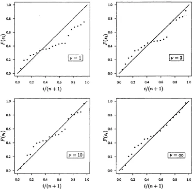
There remains the problem of assessing the adequacy of the m ultivariate t
model. This may be achieved by considering probability plots, since if Z is a
p-dimensional t(p, S , i/) random variable, then 5 = (Z — ^i)^S“ ^(Z — \Cjjp Fp,y.
Hence ‘observed’ values S{ of S may be calculated from an estim ate
(p. A),
andthe ordered values of P ( 5 < s,) may be plotted against i/( n -f-1), for i = 1, . . . , n.
3.3
E xam ples
E x a m p le 3.1. Stack-Loss data. The first example is the stack-loss data set pre
sented by Brownlee (1965). This data set has been examined by numerous authors,
including Andrews (1974), Lange et al. (1989) and, of course, Rivest (1989). As
suming th a t the 2 1 observations o n y = stack-loss, Xi = air flow, X2 = tem perature
and X3 = acid concentration may be regarded as a m ultivariate sample from a 4-
dimensional t distribution, estimates (p.y. Ay) were calculated for a broad range of
1/ values. A selection of estimates of the regression param eter (3.6) thus obtained
is given in Table 3.1. Maximised log-likelihoods are given in the second column of
the table; they describe the profile log-likelihood as a function of i/. It can be seen
th a t the m ultivariate t approach actually points to the least-squares estim ator,
given by 1/ = oo. The probability plots given in Figure 3.1 also suggest th a t the
distribution. This conclusion is quite different from th at reached by Lange et al.
(1989), who modelled the data under the assumption of univariate homoscedastic
errors, and obtained ù = 1.1. However, whether or not this represents a signif
icant improvement in fit over u = oo they leave open to question. The estim ate
given by Lange et al. is similar to th at of Andrews, and they seem to give the
best fit for the m ajority of the observations in this data set.
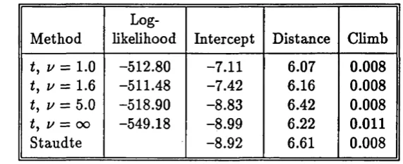
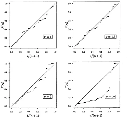
E x a m p le 3.2. Scottish Hill Races data. Staudte and Sheather (1990, pp. 265-
268) analyse a data set comprising 35 observations on a dependent variable y =
recorded tim e in minutes, and independent variables x\ = distance in miles and
X2 = climb in feet. They give generalised M -estim ates, defined as the solution to
(1.9), with w(x^) = u(x,) = (1 — hi)/y/hi and ip{ti • u(x,)) = ^c(f(/u(x^)), where
hi is the 2th diagonal element of the m atrix X (X ^X )~^X ^ and is the Huber
^-function defined in Example 1 .1 with c = kV{p + l) / n . A selection of t
M-estim ates for the data are given in Table 3.2, together with the M-estim ate obtained
by Staudte and Sheather when k = 1. The maximised log-likelihoods given in
column 2 suggest taking ù % 1.6, and this is confirmed by the probability plots
given in Figure 3.2. The largest residuals calculated from the resulting estim ate
P of the regression param eter correspond to the cases 7, 18, and 33, and are
respectively 52.9, 64.8 and 24.7 — consistent with the equivalent residuals from
the Staudte and Sheather estim ate, which are 47.8, 64.9 and 18.6.
Staudte and Sheather also consider the median of the absolute deviations from
the median (MAD) and interquartile range (IQR) of the residuals as criteria for
judging how well the fitted model agrees with the bulk of the data — small values
indicating a good fit. Their estim ate has an MAD of 3.66 and an IQR of 7.46,
whereas the multivariate t M -estim ate for i/ = 1.6 has an MAD of 3.42 and an
IQ R of 6.90, indicating a slight improvement in fit.
Finally, Staudte and Sheather note th a t the robust approach they used is
Method
Log-likelihood Intercept Air-Flow Temp. Acid
2, z/ = 1 -243.01 -35.61 0.81 0.65 -0 . 1 2
t, u = 3 -236.79 -38.19 0.82 0.81 -0.13
t, u = 10 -234.26 -39.81 0.78 1.05 -0.14
u = oo -233.15 -39.92 0.72 1.30 -0.15
Andrews -37.20 0.82 0.52 -0.07 Lange -38.50 0.85 0.49 -0.07
Table 3.1: Stack-Loss results.
1.0
-0.8
-0.6
-0.4
0.2
-0.0
-0.0 0.2 0.4 0.6 0.8 1.0
i/{n -t-1)
1.0
-0.8
0.6
0.4
-1/ = 10 0.2
-0.0
-0.0 0.2 0.4 0.6 0.8 1.0 i/{n + 1)
1.0
-0.8
-0.6
0.4
-0.2
-• /
0.0
-0.6
0.4 0.8 1.0 0.2
0.0
i / ( n - I - 1 )
1.0
-0.8
0.6
0.4
-1/ = OO
0.2
-0.0
-0.2 0.4 0.6
0.0 0.8 1.0
i/{n4-1)
Method
Log-likelihood Intercept Distance Climb z/ = 1 .0 -512.80 -7.11 6.07 0.008
tj u = 1 .6 -511.48 -7.42 6.16 0.008
(, z/ = 5.0 -518.90 —8.83 6.42 0.008
ty 1/ = oo -549.18 —8.99 6 .2 2 0 .0 1 1
Staudte -8.92 6.61 0.008
Table 3.2: Scottish Hill Race results.
This disadvantage is not shared by the m ultivariate t approach, as the degrees of
freedom param eter z/ is estim ated from the data, so th at for m ultivariate normal
d ata the least-squares estim ate can be obtained.
E x a m p le 3.3. Water Salinity data. The water salinity d ata is a widely studied
example in the robustness literature. See for example, Ruppert and Carroll (1980),
Staudte and Sheather (1990, pp. 264-265) and references therein. The data consist
of 28 observations on y = water salinity, xi = salinity lagged two weeks (sallag),
X2 = trend, which is one of the six biweekly periods in March-May, and xs =
HgO Flow — the river discharge. Various t M -estim ates for the data are given
in Table 3.3, along with a trim m ed least-squares estim ate obtained by Ruppert
and Carroll and the Staudte and Sheather estim ate with k = 2. The maximised
log-likelihoods suggest taking z) % 5, and the outlying cases are then 15, 16 and
17 — with residuals of -2.38, 5.68 and -2.20, broadly agreeing with the results of
R uppert and Carroll and Staudte and Sheather. Note th at the t M -estim ate of P
is very similar to the estim ate given by Staudte and Sheather, and both are quite
different from least squares.
In both of the studies cited above the MAD and IQR of the residuals are
considered as means of comparing the fit of competing estim ates. The MAD
and IQ R of the t M -estim ate given by z/ = 5 are respectively 0.45 and 1.06,
1.0
-0.8
-0.6
0.4
-0.2
-0.0
-0.6 0.8 1.0
0.0 0.2 0.4
*7(n + 1)
1.0
-0.8
-0.6
0.4
-0.2
-0.0
-0.0 0.2 0.4 0.6 0.8 1.0
i/{n + 1)
1.0
-0.8
-0.6
0.4
-u = 1.6 0.2
-0.0
-1.0
0.6 0.8
0.0 0.2 0.4
* / ( n + 1 )
1.0
-0.8
0.6
0.4
-0.2
-0.0
-0.8 1.0
0.4 0.6
0.0 0.2
i/{n + 1)
Figure 3.2: Probability plots for Scottish Hill Race data.
Method
Log-likelihood Intercept Sallag Trend Flow
1/ = 1 -239.40 20.15 0.707 -0.173 -0.704
t, u = 3 -233.06 18.87 0.715 -0.166 -0.653
t, u = 5 -232.50 17.56 0.723 -0.148 -0.601
ty u = 7 -232.68 16.46 0.729 -0.131 -0.558
t, 1/ = oo -235.75 9.59 0.777 -0.026 -0.295
Ruppert 14.49 0.774 -0.160 —0.488 Staudte 16.89 0.715 -0.142 -0.570
R uppert and Carroll for their estimates. Therefore in terms of these criteria the
t M -estim ate compares very favourably with those obtained from other robust
methods.
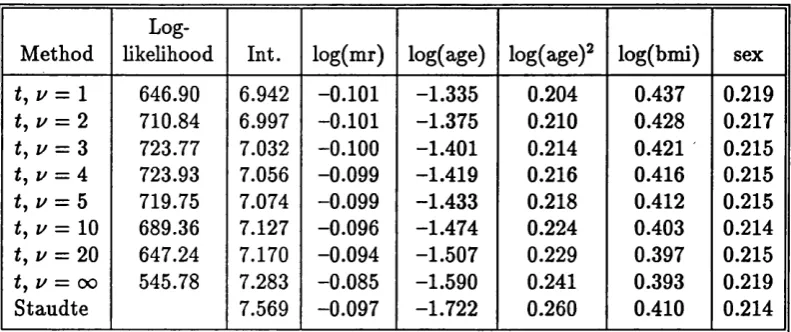
E x a m p le 3.4. Twickenham Run-Times. This is a much larger data set, consist
ing of the finishing times of 556 runners (472 male, 84 female) who completed
an 8 mile race in Twickenham, England, in 1983. For each individual there are
measurements on the following:
y = log (finishing time), x\ = log (miles run per week 4-1), X2 = log(age),
xz = log( weight), 2:4 = log (height),
a = number of other active sports per week (0, 1, or 2), and
s = sex ( 0 = male, 1 = female).
A “body mass index” variable xs = log(weight/height^) is also defined. For sim
plicity, the runners who gave only partial information have been om itted.
We seek a simple linear model relating finishing tim e to the various explana
tory variables, and a conventional m ultiple regression model selection procedure
suggested the following:
2/ = ^ 0 + + ^2^2 + ^z^2 d" ^42:5 + PsS + e.
The data cannot be regarded as a random sample from a m ultivariate t distribu
tion, particularly as both X2 and x\ are included in the model, but nevertheless,
m ultivariate t M -estim ates of the regression param eter are given in Table 3.4.
For comparison, we also include the estim ate obtained by using the Staudte and
Sheather m ethod with k = 1. The results suggest th a t the log-likelihood is max
imised with % 4. The difference in log-likelihood between the best fitting t and
the normal model yields a likelihood ratio chi-squared statistic of 356.3 on 1 df, an
apparently significant improvement in fit. However, there is a negligible difference
in term s of the MAD and IQR: for the t, u = A model we obtain an MAD of 0.066
Method
Log-hkelihood Int. log(mr) log(age) log(age)2 log(bmi) sex
tj 1/ = 1 646.90 6.942 -0 .1 0 1 -1.335 0.204 0.437 0.219
t, u = 2 710.84 6.997 -0 .1 0 1 -1.375 0 .2 1 0 0.428 0.217
(, z/ = 3 723.77 7.032 -0 .1 0 0 -1.401 0.214 0.421 0.215
t, u = A 723.93 7.056 -0.099 -1.419 0.216 0.416 0.215
f, z/ = 5 719.75 7.074 -0.099 -1.433 0.218 0.412 0.215 i, z/ = 1 0 689.36 7.127 -0.096 -1.474 0.224 0.403 0.214
u = 20 647.24 7.170 -0.094 -1.507 0.229 0.397 0.215
ty u = oo 545.78 7.283 -0.085 -1.590 0.241 0.393 0.219
Staudte 7.569 -0.097 -1.722 0.260 0.410 0.214
Table 3.4: Twickenham Run-Time results.
0.067 and 0.133. The Staudte and Sheather estim ate yields the same values for the
MAD and IQR as the u = A estim ate, and so it appears th at the least-squares
estim ate is adequate for this d ata set.
To examine whether or not the indicator variable for the sex factor has had an
undue influence on the estim ate z), separate estimates for males and females are
also presented in Tables 3.5 and 3.6. For males only, z / 5, and for females, z/ % 4. It seems therefore th at the estim ate of v obtained for the combined data has not
been largely influenced by the inclusion of an indicator variable. The MAD and
IQR for the f, z/ = 5 male estim ate are 0.065 and 0.130; for the f, z/ = 4 female
estim ate they are 0.075 and 0.153; the corresponding figures from the Staudte and
Sheather estim ates are 0.063, 0.127 and 0.074, 0.154.
Probability plots are given in Figure 3.3. The plot for z/ = 4 is quite good,
save for the noticeable discrepancy at z/(n -|- 1) % 0.8, which may be due to the
univariate probability plot obscuring the fact th at the data are not m ultivariate
t. The z/ = 4 plot is not, however, as good as the univariate normal probability
plot for the least-squares estim ate (not shown), which indicates no departure from
Method
Log-likelihood Int. log(mr) log(age) log(age)2 log(bmi)
t, u = 1 637.86 6.925 -0 .1 0 1 -1.326 0.203 0.436
= 3 764.90 6.992 -0 .1 0 0 -1.381 0 .2 1 1 0.418
t, 1/ = 4 774.99 7.016 -0.099 -1.400 0.214 0.412 1/ = 5 777.38 7.034 -0.098 -1.415 0.216 0.407 1/ = 6 776.34 7.048 -0.098 -1.423 0.218 0.404
t, u = oo 659.13 7.083 -0.083 -1.502 0.229 0.359
Staudte 7.527 -0.096 -1.704 0.257 0.405
Table 3.5: Twickenham Run-Time results — Males only.
Method
Log-likelihood Int. log(mr) log(age) log(age)2 log(bmi)
t, 1/ = 1 135.47 5.644 -0.098 -0.534 0.088 0.323 1/ = 3 155.06 6.345 -0.103 -0.904 0.140 0.360
t, u = 4 155.55 6.543 -0.104 -1.004 0.155 0.376
ty u = 5 154.82 6.683 -0.105 -1.072 0.164 0.391
t, u = Q 153.64 6.784 -0.106 -1.119 0.171 0.403
t, u = oo 120.34 7.698 -0.107 -1.540 0.231 0.555
Staudte 7.020 -0.109 -1.233 0.187 0.427
1.0
0.8
0.6
0.4
0.2
0.0
0.0 0.2 0.4 0.6 0.8 1.0
i/{n + 1)
1.0
0.8
0.6
0.4
i/ = 20 0.2
0.0
0.0 0.2 0.4 0.6 0.8 1.0
1.0
0.8
0.6
0.4
1/ = 4 0.2
0.0
0.0 0.2 0.4 0.6 0.8 1.0
i/{n + 1)
1.0
0.8
0.6
0.4
1/ = OO
0.2
0.0
0.0 0.2 0.4 0.6 0.8 1.0
i/(n + l) *7(n + l)
3.4
C onditional
t
A f-estim ates
3.4.1 M ain R esu lt
For many data sets, such as those arising from designed experiments and those
involving curvilinear term s such eis Example 3.4 discussed earlier, it is not rea
sonable to impose a m ultivariate t framework on the covariates. In such cases it
would be preferable to estim ate directly the conditional distribution of a response
y given a set x of explanatory variables, i.e., without regard to the joint marginal
distribution of x. This is effectively what occurs in conventional least-squares re
gression, which can be viewed as a m ethod for estim ating a conditional normal
distribution.
Unfortunately, this approach breaks down when we consider the conditional t
distribution, for as we prove in this section, it yields a highly nonregular likelihood
function, being, in general, singular at each of the d ata points. The likelihood is
thus intrinsically multimodal, with modes of infinity, so th at unrestricted maxi
m um likelihood estim ation breaks down. We proceed as follows.
The conditional t M -estim ate of |3 is the estim ate defined by (3.6), but with
its component terms obtained by maximising the log-likelihood function corre
sponding to the conditional distribution of Z1IZ2 = Z2, rather than the full joint
distribution of Z% and Z2. DeGroot (1970) notes th a t the conditional distribution
is a Pi-dimensional t distribution on 1/1.2 = ^-\-p2 degrees of freedom, with location
param eter jx given by (3.5) and scatter m atrix
S = Pt/(Z2, P2, S22) S 1.2,
where
M2, S22) = i^i.2 { y + (Z2 — M2)^S^(Z2 — M2)}
constant involving only U\ . 2 and pi, is given by
= - 1 log IÊ.I - 1 I (z ii - - M .)}, (3.7)
1=1 t=l ^ ^
where \ii and S,- are respectively \i and S evaluated at Z2 = Z2*. For the linear
model, we have Z2* = x,-, fh = ( 1 x f ) P and we may denote S1.2 and È,- as,
respectively, cr^ and a f, where a f = ^^(x^, P2» S22)
Ideally, maximisation of the full log-likelihood Lz(li, S , z/) as carried out in
Section 3.2 would be equivalent to maximisation of the conditional log-likelihood
^Zi|Z2(l^j so th at the results on existence and uniqueness may still apply.
This is true for the m ultivariate normal {v = 0 0) case, as can be shown by writing
T z (li,S ,z /) as
^ z (p , S , z/) = 4- ^2 2(112, ^ 22,%/),
where Tz2(li2, S2 2, is the log-likelihood corresponding to the marginal distri
bution of Z2. In the normal case, it is easy to show th at the marginal compo
nents (corresponding to the marginal distribution of Z2) of the maximum likeli
hood estim ate (p, S ) for the full log-likelihood are the maximum likelihood esti
mates (p2, S22) for the marginal log-likelihood. It follows th a t the derivative of
-^Zi|Z2(l^)S) with respect to \i and S must equal 0 at the value (p, 2 ) = (A ,S ),
and so for infinite z/, maximising the full likelihood is equivalent to maximising the
conditional likelihood. For finite z/, this is not the case, since the conditional like
lihood contains information about P2 and S22. This difficulty is, however, minor
in comparison to the more fundam ental existence problem given in the following
theorem. Before presenting the theorem, however, it is convenient to make a minor
change to the notation, by denoting the num ber of occurrences of an observation
Z2i in a given data set as r,-.
T h e o re m 3.1. For a data set {z,- = (z^ z^ J^ E i = 1 , . . . ,n }, the condi