© 2015 IJSRST | Volume 1 | Issue 3 | Print ISSN: 2395-6011 | Online ISSN: 2395-602X Themed Section: Engineering
Design of Classical and State Space Controller Using a Moving
Coil Machine
Folayan Gbenga, Adeoye O. S.
Department of Electrical and Electronic Engineering, Federal Polytechnic, Ado-Ekiti. Ekiti State, Nigeria
ABSTRACT
This paper looks at two methods of designing controllers among numerous approaches used in controller designs; the root locus method using the SISOTOOL in MATLAB and the state space method. The root locus is a classical graphical method, of all the classical methods this was chosen because it helps to understand fundamental concept of controller design, and a graphical understanding of what is going on in the system. This paper analyse, design, compare and contrast a classical method, PID and a more recent approach; state space to controller design. The state space approach is more modern and used to highlight the short comings of the classical approach. A laboratory moving coil meter was used for the design of the controller. The utilisation of the system identification toolbox in MATLAB was employed for the system modelling obtained and analysed. Finally the paper compares the performance of both designed controllers based on root locus and state space methods at the second order moving coil system and previous work done were subjected to due comparison.
Keywords: Controller, Root Loci, State Space, MATLAB, Model and Moving coil meter.
I.
INTRODUCTION
The paper tends to make the difference between the classical and a more modern approach in the design of controllers. When we have a system, we want that system to behave in a desired manner. But that is often not the case as external signals often known as noise interferes with the system and therefore an output less than the desired.
The need for a method to make the system behave in the desired manner leads to the development of control engineering. Control engineering involves the design of an engineering product or system where a requirement is to accurately control some quantity (Dutton, K 1997). The system used in this paper is the moving coil machine. The moving coil machine is used to measure current. Whenever electrons flow through a conductor, a magnetic field proportional to the current is created. This effect is useful for measuring current and is employed in many practical meters (Kim, 2006). To use a permanent –magnet moving coil device as a meter two problems must be solved. First, a way must be found to
compensation method. The root locus method is adopted in this paper without any specific reason.
After the introduction we have the methodology where the root locus and the state space methods are discussed followed by the discussion of results obtained and finally the conclusion.
II.
METHODS AND MATERIAL
The methods employed in the design of controllers for the moving coil machine is the root locus approach and the state space method. For certain systems, their properties are described using graphical models which use numerical tables and plots. That means for linear systems, they are describing by their step or impulse responses and or by their frequency function. For more advanced applications , models that describe the relationship among the system variables in mathematical expressions like differential equations are used which could be time continuous or time discrete, lumped or distributed, deterministic or stochastic, linear or non-linear as well as the graphical method. The third method uses the experimental approach. Here experiments are carried out on the system and a mathematical model of the system can be found. This is known as system
identification and it includes the following;
Experimental planning, Selection of model structure, parameter estimation and Validation (Dutton 1997). This method is used for the purpose of this paper. The experimental design involves several factors. The choice of the input signal and choice of sampling interval is of great importance. In a system identification experiment, the input signal applied to the system can have great influence on the resulting parameter estimates. The major types of input signal used in system identification experiment are; Step function, Steady input (static test), Impulse input and Random input-Pseudorandom binary sequence. A pseudo-random-binary-sequence (PRBS) is a two state signal of logic 1 levels and logic 0 levels. Logic 1 will be a positive voltage and logic 0 an equally negative voltage. It can be generated by using a feedback shift register. It cannot be said to be truly random since it repeats itself every 2n-1 bit interval for
an n-bit shift register (SoderstrÖm and Stoica, 1989).
Inappropriate model structure is the most common cause of problem in system identification. Optimum model structures which have just sufficient parameters are
needed to model the process. There are numerous time series model but for the purpose of this paper the (ARMA) model is used. Auto Regressive model is one where the current value of a time variable is a function of its past values only. In other words the current output is a weighted sum of previous output values. It is auto regressive because its form shows a regression of a time variable with itself at different time instants (Tham, 1999).
It is generally represented as:
...1 defines the oldest output value that has a significant influence on the current output. The Moving average model believes that its output is dependent upon the current state of the input and what that input was doing for some time in the past represented as:
... 2
A more realistic model would have been to consider both the input and output because practically the output of the system is a function of both the input and outputs.
AR+
MA ... 3 ARMA
The background knowledge of the system made it easy to make decisions on the model and to estimate its parameters. The system is a linear second order under damped system, and because a continuous transfer function is preferred as the system representation, the choice of process model in system identification of MATLAB is not a difficult choice to make. Having
specified the characteristics, the mathematical
representation is obtained:
...………4
state space description to enable manipulation. A new mathematical model is obtained in discrete form to avoid converting from the continuous form to discrete form. This is to avoid the unnecessary uncertainties in the obtained result.
Using the same process used in obtaining the mathematical model for the system in the earlier section of identification. Using linear parametric models, specifying ARX as the structure, using 2,2,1 as the order and instrumental variables as the method we obtain
( )
...5
Verification shows that the transfer function truly represents the system.
Thecontroller must be able to do the following: correct
the steady state error, improve the speed of response that is rise time and settling time, stability and better oscillation i.e. the percentage overshoot and damping ratio. Proportional action takes corrective action based on magnitude of the error and integral takes corrective action based on the area under the error curve. This means that when error rapidly changes when the magnitude has not changed much then P+I will not give much corrective action. The inclusion of the integral action only is not good enough so we need a third term that will make control signal proportional to the time derivative (rate of change) of the error signal
( ) ( )
...6
Where Kd is the derivative gain.
Root Loci Design
The root locus plot is the plot of the s zero values and the s poles on a graph with real and imaginary coordinates. The root locus is a trace of the spots of the poles of a transfer function as the gain K is varied. The locus of the roots of the characteristic equation of the closed loop system as the gain varies from zero to infinity gives the name of the method. Such a plot shows clearly the contribution of each open loop pole or zero to the locations of the closed loop poles. This method is a very powerful graphical technique for investigating the effects of the variation of a system parameter on the locations of the closed loop
poles. Sketching root loci is simple if the general rules for constructing is followed. “The closed loop poles are the roots of the characteristic equation of the system. From the design viewpoint, in some systems simple gain adjustment can move the closed loop poles to the desired locations. Root loci are completed to select the best parameter value for stability. A normal interpretation of improving stability is when the real part of a pole is further left of the imaginary axis”. (Roy 2010).
State Space Design
The state space approach is a more modern approach to controller design. It is a unified method for modelling, analysing, and designing a wide range of systems. In the recent past there have been a number of developments and papers written about true digital control (TDC) design, in which discrete time is used in the design of control systems. TDC is actually based on simplified
refined instrumental variable identification and
estimation algorithms for data based modelling (Young, 2004) and later the design of Proportional Integral Plus (PIP) control algorithms (Young et al 1987).
A proportional integral plus (PIP) controller is a full discrete state variable feedback controller based on non-minimal state space description (NMSS). NMSS follows methodological approach from earlier research. Hesketh (1982), Young, Behzadi, Wang & Chotai (1987), in which NMSS models are formulated so that, in the deterministic situation, full state feedback control can be implemented directly from the measured input and output signals of the controlled process, without resort to the design and implementation of a state re-constructor (or observer). This yields a PIP design that is naturally robust to uncertainty and eliminates the need for measures such as loop transfer recovery.
The mathematical editor on which along with text you can also write
III.
RESULT AND DISCUSSION
Using SISOTOOL on MATLAB to achieve the design requirements we add a complex zero and adjust the gain. Reading off the compensator values from the SISOTOOL we obtain equation 7
Gcs=4.59351s+0.65+0.412s ……….. 7
Rearranging and writing in form of a PID transfer function, that is;
Gcs=Kp1+1sTi+sTd ……… 8
We have
Gcs=2.9861+10.65s+0.2586s ……… 9
Having; Kp=2.986;
Ti=0.65;
Td=0.2586.
Figure 1: Simulink model used to obtain system data
Figure 2: Obtained PID being tested on the model and system
Figure 3: Response to a step input. Downward because of the negative transfer function
The difference equation gives for equation 5 gives:
( )
... 10
Considering the State Space equation;
̇ = ( Xk+1 = A Xk + BUk ) ...11 ...12
Where the state vector is a column vector of length n;
Input vector u is a column vector of length r; A is an n x
n square matrix of constant coefficients; B is an n x r
matrix; Y is a column vector of the output variables; C is
an m x n matrix of the constant coefficients that weight
the state variables and D is an m x r matrix of the constant coefficient that weights the system inputs.
And to obtain our non-minimal state space
representation,
( )
... 13
[
]
[
] [
] +
[
] UUn ………14
the above matrix include an integral of the error state.
Comparing the above expression to equation 9 we can
say that;
A=[
]
B= [
]
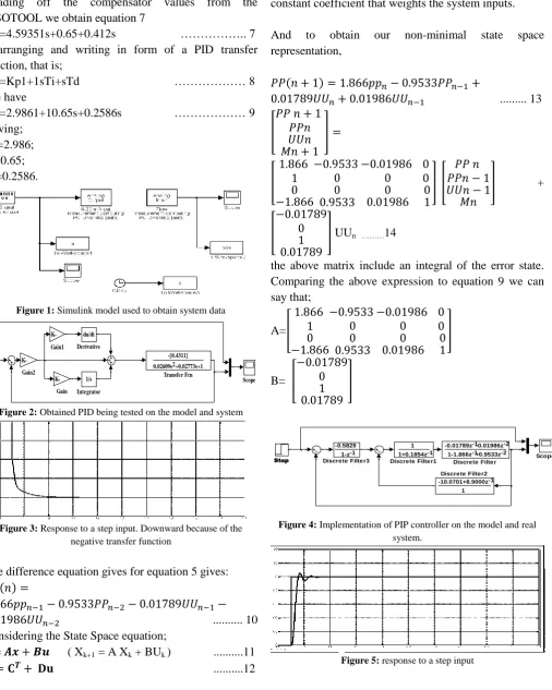
Figure 4: Implementation of PIP controller on the model and real system.
Figure 5: response to a step input
-[0.4311]
0.02609s +0.02773s+12
Transfer Fcn Step1
Scope 1/s
Integrator
-K-Gain2
-K-Gain1
-K-Gain du/dt
Derivative
Step Scope
-0.5829 1-z -1 Discrete Filter3
-10.0701+8.9000z -1 1 Discrete Filter2 1
1+0.1854z -1 Discrete Filter1
-0.01789z -0.01986z -1 -2 1-1.866z +0.9533z -1 -2
The design carried out to obtain Fig.3 using root locus considered steady state error and transient response. The design method was iterative. Iterating around the design specifications changing the design and checking the response until the result is deemed acceptable. The approach has the difficulty in detecting if the system is controllable or not while the designer labour over a long period of time before coming to such conclusion.
The design of state variable systems feedback (SVF) is a very different approach. The desired closed loop performances are specified in advance and together with the state space model of the open loop plant are fed into an algorithm (an m.file in MATLAB) the algorithm then produces the details of the required controller.
To be able to design the necessary a controller for our dynamic system the system must be controllable. In other words it must be possible to move all of the system open loop poles by state variable feedback to any arbitrary closed loop locations.
IV.
CONCLUSION
Thispaper has looked at two approaches to analysis and
design of feedback control system. The first part looked at the classical approach. This method uses root locus and the MATLAB SISOTOOL, by obtaining a model of the system and analysing its poles and zeroes.
The main advantage of the method is that they readily provide the stability and transient response information so it is easy to see the effect of adjusting the poles and zeroes until an acceptable design is met.
However the main disadvantage lies in the fact that its usability is limited. It can only be useful for linear time invariant systems or system that can be approximated as such.
The second method used a more recent approach to system control. This method cannot only be used for same class of systems as classical method but also analyse non-linear systems that have backlash, saturation and dead zone. It can also model systems with non - zero initial systems as well as multiple input multiple output (MIMO) systems.
One of the draw backs of frequency domain method of design using either root locus or frequency domain is that after designing the location of the dominant second order pair of poles , we keep our fingers crossed, hoping that the higher order poles do not affect the second order approximations. Frequency domains methods do not allow us to specify all poles in the systems of order higher than 2 because they do not allow for a sufficient number of unknown parameters to place all of the closed loop poles uniquely. One gain to adjust, or compensator pole and zero to select, does not yield a sufficient number of parameters to place all the closed loop poles at desired location. To place n unknown quantities, you need n adjustable parameters.
State space method solves this problem by introducing into the system
(1) Other adjustable parameters and
(2) The technique for finding these parameter values, so that we can properly place all poles of the closed loop system.
On the other hand, state space methods do not allow the specification of closed loop zero location, which frequency domain method do allow through placement of the lead compensator zero. This is a disadvantage of the state space methods, since the location of the zero does not affect the transient response. Also, a state space design may prove to be very sensitive to parameter changes.
Finally there is a wide range of computational support for state space methods; many software packages support the matrix algebra required by the design process. However as mentioned before the advantages of computer support are balanced by the loss of graphic insight into a design problem that the frequency domain methods yield.
V.
REFERENCES
[1] Astrom K. and Hagglund T., (1994) PID Controllers: Theory, Design, andTuning. Research Triangle Park, NC: Instrument Soc. Amer.
[2] Beadmore R. (2010) Root Locus Analysis of Control
systems,[online], available at
[3] Cheng, L., Hou, Z.G., Tan, M., Liu D., and Zou, A.M. (2008) Multi-agent based adaptive consensus control for multiple manipulators with Kinematic uncertainties, pp. 189-194 [4] Dutton K., Thompson S., Barraclough B. (1997), The Art of
Control Engineering, Essex: prentice hall.
[5] French, I (2009), System Identification and Adaptive Control Lecture Note, Teesside University, Uk
[6] Hesketh T., (1982). State-space pole-placing self-tuning regulator using input-output values. IEE Proceedings 129 4D (1982), pp. 123-128
[7] Jun Gu, James Taylor & Derek Seward (2004); Computer-Aided Civil and Infrastructure Engineering Proportional-Integral-Plus Control of an Intelligent Excavator.
[8] Ljung L. (1987) system identification Theory for the user. London. Prentice hall. Inc.
[9] Mestha L.K. & Planner C.W. (n.d). Application of system identification techniques to an RF cavity tuning loop. [online] available at: http://lss.fnal.gov/archive/other/ssc/ssc-n-706.pdf [13 march 2010].
[10]Norman S. Nise (2008) Control Systems Engineering 5th edition asia: john Wesley and sons.
[11]Soderstrom T., Stoica P. (1989),system Identification New jersey, prentice Hall
[12]Taylor C. J., Leigh P., Price L., Young P. C., Vranken E. and Berckmans D. (2004) Proportional-integral-plus (PIP) control of ventilation rate in agricultural buildings control engineering practise 12(2) [online] available at:
http://www3.interscience.wiley.com/cgi-bin/fulltext/118801781/PDFSTART
[13]Tham M.T. (1999) Dynamic Model for Controller Design,
[online], available at
http://lorien.ncl.ac.uk/ming/digicont/mbpc/models.pdf [accessed12 march 2010].
[14]The Mathworks (2010) System Identification tooolbox [online]
available at:
http://www.mathworks.com/access/helpdesk/help/toolbox/ident/ gs/bqv54ev-7.html. [accessed on 15 march 2010].