Fe Coefficient – Development and Application of a Key Figure for Assessing the Efficiency of Alternative Drive Concepts in Trucks

(1)

http://www.sciencepublishinggroup.com/j/ajtte doi: 10.11648/j.ajtte.20190402.12

ISSN: 2578-8582 (Print); ISSN: 2578-8604 (Online)

Fe Coefficient – Development and Application of a Key

Figure for Assessing the Efficiency of Alternative Drive

Concepts in Trucks

Klaus-Peter Franke

Institute of Industrial Engineering and Supply Chain Management, Ulm University of Applied Sciences, Ulm, Germany

Email address:

To cite this article:

Klaus-Peter Franke. Fe Coefficient – Development and Application of a Key Figure for Assessing the Efficiency of Alternative Drive Concepts in Trucks. American Journal of Traffic and Transportation Engineering. Vol. 4, No. 2, 2019, pp. 48-55.

doi: 10.11648/j.ajtte.20190402.12

Received: March 26, 2019; Accepted: April 28, 2019; Published: May 23, 2019

Abstract:

Alternative drive concepts for trucks represent a highly promising way of reducing environmental pollution from road freight traffic. There are numerous proposals and pilot schemes pointing to the replacement of fossil fuel diesel by more sustainable energy sources. Along with drive chain electrification, it is a matter here of deploying alternative natural (gas) and synthetically generated fuels (eFuels) in combustion engines that might have to be modified. Given that a multitude of parameters on final energies, vehicle and travel route/ ambient conditions enter into the consumption calculation, it is usually difficult to compare the various drive concepts based on individually gauged consumptions/emissions. It is therefore proposed assessing the comparison on the basis of the same vehicle platform under practically the same deployment and route parameters. In other words, in order to examine an alternative energy as to its efficiency, only the vehicle drive chain is replaced - everything else remains as it is! The Fe coefficient in the heading is formulated to afford a simplified comparison of the various drive concepts under the above general conditions. Going into the Fe coefficient in each instance is solely the mean drive efficiency over the route ηE-N and the payload to total load ratio under full capacity utilisation ηkon (design efficiency).

The calculated Fe coefficient provides information on consumption. The greater the Fe the higher the consumption. Under the same vehicle platform - and with consideration given to the above general conditions - the Fe coefficients of the various drive variants can be related one to the other and, in this way, the increase or decrease in consumption as against, for instance, the diesel benchmark can be established. In conclusion, the Fe coefficient is used in three case studies to assess the effectiveness as against the diesel benchmark of two electric battery (Fuso eCanter, Tesla Semi) trucks and one LNG-driven Iveco Stralis NP 400 truck.

Keywords:

Transport Logistics, Road Freight Traffic, Transport Efficiency, Energy Demand Calculation, Fe Coefficient

1. Introduction

Traffic contributes significantly to the worldwide consumption of fossil energies and associated environmental pollution. For instance whilst in Germany the non-traffic sectors contributed to the German climate protection plan being met between 1990 and 2014 by lowering the anthropogenic CO2e-emissions from 1.248 billion tons to

0.902 billion tons, the 0.160 billion ton share of the traffic sector remained practically constant [1-2]. Irrespective of the fact that both private and goods traffic have exceeded local pollutant limits for years now and that diesel vehicles will be

banned from city centres at some point in the future [3], the German government is requiring traffic-induced CO2

e-emissions to be reduced to under 0.098 billion tons by 2030 [1]. Thus a lot needs to be done to bring about environmentally compatible traffic conditions in the remaining 11 years. As such, both the vehicle industry and the road haulage/logistics sector are currently busy working on a number of points for the improvement of transport and fuel efficiency. The up-and-coming innovations basically follow the three mega trends of automation, digitalisation and alternative drives [4].

(2)

(Chapter 2) as to their efficiency is an intricate business. In this respect, the idea in Chapters 3 and 4 is to devise an efficiency coefficient (Fe coefficient) permitting an easy assessment to be made of the efficiency of alternative drive chains in the given truck under the same vehicle and route parameters. The following case studies focus on electric battery trucks and those with LNG engines. The purpose of the Fe coefficient is to assess the efficiency of the 7.5 ton Fuso eCanter (Chapter 5), the Tesla Semi (Chapter 6) and the 40 ton Iveco Stralis NP 400 (Chapter 7) over their diesel counterparts and, in this way, to contribute scientifically to the current pro & contra discussion. The article closes with a summary, critical reflection and an outlook (Chapter 8).

2. Alternative Drives in the Truck

2.1. Overview

The alternative truck drives subject is focussed on changing the energy source away from mineral oil - as the scarce and environmentally damaging primary energy source - towards

1.Replacing diesel fuel in (correspondingly modified) combustion engines with less ecologically damaging alternative fuels like CNG (compressed natural gas with a 90% + methane share), LNG (liquefied methane), oxygen and CO2-neutral synthetic fuels or

2.Replacing combustion engines with electric motors with electrical energy generated when the truck is moving from hydrogen (fuel cells), supplied by way of current collectors from overhead lines or carried along in batteries. Differences in the provision and/or storage of the energy source (overhead line, fuel cells, batteries, tanks for liquids, pressure tanks for gases, cooling), type of engine (combustion engine, el. motor) and drive unit (mechanical, hydrostatic, electric) plus differences in the energy densities of the energy supply possibly carried along result in differences in the net weight and/or permitted payload as well as different efficiencies in transforming final energy into motion energy. Having to consider all these factors can make a comparison of the vehicle efficiencies a highly intricate one.

2.2. Electric Battery Drives

Whilst cars with electric drives - either as hybrids or fully electric cars - have been coming from the belt for some years now, e-trucks are either still at the prototype stage or have just left it. Only as expensive conversions have e-trucks been in evidence up to shortly ago. That has involved removing the combustion engine-driven drive chain and replacing it with an electric drive chain. But things have also been happening here. Mitsubishi Fuso has seen its electric battery eCanter (7.5 tonner) coming off the belt in a pilot batch (550 all told) [5]. And its competitors (Daimler, MAN etc.) are also about to catch up. Given that up to the fall of 2017 only electrifying distributor trucks of a moderate range and a high stop-and-go share seemed feasible, the surprise was

considerable on learning in November 2017 that Tesla planned to bring an electric battery long-distance truck (Tesla Semi) of a total 36.29 t weight and an 800 km range onto the market in 2019 [6].

There is considerable speculation on the merits and drawbacks of electric battery trucks as replacements for diesel vehicles. On the one hand, it involves how electrical energy, if at all, can be provided nationwide and more or less quickly “tapped”, on the other, of how practical and efficient electric utility vehicles really are compared to diesel trucks or those run on alternative energies. The last question will be gone into with the example of the Fuso eCanter and the Tesla Semi.

2.3. Gas Engines for the Combustion of LNG and CNG

Iveco, Scania (Otto principle) [7] and Volvo (HPDI principle) are equipping heavy trucks with gas engines [8]. The prime functional difference of interest here between engines operating on the basis of the Otto principle and those on the basis of the HPDI principle (High-Pressure Direct Injection) is their efficiency ηe,opt. [18, S. 20] indicates that fuel efficiency in engines functioning on the basis of the Otto principle is down by 15 to 25% as against diesel whilst in [9, Page XVI] the talk is of where optimized natural gas engines functioning on the basis of the Otto principle they should ideally be able to attain up to 95% of diesel efficiency. Should Iveco’s announcement of its new Stralis NP 460 having “up to 15% lower fuel consumption” also relate to comparable gas engines, then the new Cursor 13 NP engine has an efficiency surpassing 90% of a comparable diesel unit. In contrast, HPDI engines (self-igniter i.e. „liquid spark plug“) have a fuel consumption which energetically is at the same level as for conventional diesel engines [9, S. 63]. Basically, both process principles allow the use of LNG and CNG although the engines have to be adjusted to the way in which the natural gas is provided.

(3)

km with CNG and LNG respectively for its fully loaded Stralis NP460 [19, S. 15].

3. The Energy Demand Calculation

Theory

3.1. Modelling

The (final) energy consumption EE of a truck (Formula 1) is conditional upon the work (corresponds to the effective energy to be provided EN) which the vehicle has to perform along a distance s between source and sink for overcoming the external motion resistances Fges = Fmass + Faer with consideration given to an efficiency ηE-N (cf. [10]).

= ∙ [ + ] ∙ (1)

The across-the-route s variable efficiency ηE-N of the power transmission between the input of final energy from the tank and the provision of effective energy to the drive wheels considers the efficiencies ηE-mot between energy reservoir and engine, ηmot = ηe of the engine as well as ηmot-N between engine and drive wheels (Formula 2)

= ∙ ∙ (2)

By dispensing with the integer spelling and by entering mean values over distance s Formula 1 can be transferred into Formula 3. The increase of the energy consumption EE

due to a divergence of efficiency ηE-N, i.e. principally that of the share ηmot of the efficiency , at the ideal operating

point, is taken into account by a (drive line) factor α1. It can also consider consumption increases due to non-ideal operations e.g. constant crawling speed under internal company transport operations.

= ∝

, !"∙ [ # + # ] ∙ (3)

The mass-dependent mean motion resistance # is calculated (Formula 4) by a (route) factor α2, the rolling

friction coefficient µR, gravitational acceleration g and the masses from vehicle net weight mEG and payload mNL.

# _{= $}_%_{∙ µ}_'_{∙ ()} _*_{+ )} ₊_{) ∙ -}₍₄₎

Factor α2 takes into account (Formula 5) the share transformed into heat from braking along the distance s after accelerating and/or surmounting inclines by applying a mean fictitious acceleration .# and/or mean fictitious incline /0. The effect of not converting any energy into heat from braking e.g. when travelling at a constant speed on the level, as a consequence, produces $% = 1 . $% is reduced when

kinetic/potential energy placed beforehand into the system is recuperable under braking conditions.

$

_%

=

23

∙ (

#

4

+ 5

'

+ /0)

(5)

The mean air resistance # arises (Formula 6) from the

air density ρL = 1.2 kg/m³, the product of cross-section area A

and air resistance coefficient cW of the truck and the mean vehicle speed 60. The impact of wind is negligible!

#

_{= 0,5 ∙ 9}

₊

_{∙ : ∙ ;}

_<

_{∙ 60}

%

(6)

3.2. Discussion of Vehicle Parameter α1 and Road

Parameter α2

The effect of using Formula 4 for the mass-dependent mean motion resistance # in Formula 3 and cancelling it as per α1 produces the connection between α1 and α2 under given energy consumption EE (Formula 7).

∝ = ∙ , !"

[ ∝₌ ∙>₃∙( _?@ _A)∙4@B#_CDE] (7)

By plotting α1 via α2, the possible value pairs (α1, α2) for a given energy consumption EE would create a sub-linear hyperbola course in the top right quadrant of an axis cross with origin (1, 1). The maximum of α1 arises for α2 = 1 and vice versa. The higher the consumption, the further away the hyperbola is from the origin and/or the larger become the maxima of α1 and α2.

In [11] the consumption of six fully loaded articulated lorries (40 t, Euro-6 standard), which the VerkehrsRundschau tested on a five route-sectioned course of varying difficulties from 2014 to 2016, was analysed with Formula 3. The mean values for α1,max (for α2 = 1) of the six trucks lay between 1.17 (easy-to-negotiate autobahn) and 1.75 (road) whilst the mean values for α2,max (for α1 = 1) of the six trucks lay between 1.39 (easy-to-negotiate autobahn) and > 1.89 (road).

3.3. Formulation of a Vehicle Efficiency Coefficient Fe

Vehicle efficiency is to be assessed for full capacity utilisation on the basis of the specific (final) energy consumption eE in kWh per transported ton of payload and km. Following change-over and introduction of a design efficiency F G, Formula 3 can be transferred into Formula 8.

A,HIJ ∙ =

K

, !" ∙ L M∙

[B#NCOO@B#CDE]

PDO,HIJ = Q (8)

The design efficiency F G stipulates the ratio of

maximum permitted payload ) +,RSTto max. permitted total

weight )4 ,RST = ) *+ ) +,RST (Formula 9). The larger

the F G, the smaller is the dead weight mEG to be moved. For

instance, tanks / batteries with energy sources of a comparable low energy density result in a significant increase in vehicle weight mEG when substantial vehicle ranges are to come about. Furthermore, the net weight of pressure tanks, e.g. for storing liquid hydrogen, should not be underestimated.

F G= A,HIJ

PDO,HIJ (9)

(4)

Q = Q ∙[B#NCOO@B#CDE]

PDO,HIJ (10)

To be entered into the vehicle efficiency coefficient Fe is the power provision efficiency under optimum operating conditions , , factor $ and design efficiency F G

(Formula 11).

Q =

K

, !" ∙ L M (11)

The vehicle efficiency coefficient Fe enables drive variants to be tested (for the first time) under the same vehicle (especially aerodynamics, tyres, permitted total weight) and route parameters (especially height profile, speed profile, weather conditions) The smaller the Fe, the lower the specific energy consumption eE or the higher is the vehicle efficiency per tkm under given vehicle and route parameters.

4. Case Study 1 – Fuso eCanter

The Fuso eCanter is the first line-produced electric battery 7.5 tonner. It is fitted to the chassis of the corresponding diesel version (FE 160) of the Fuso Canter, which is assembled in Portugal [5, 12].

On the basis of the vehicle efficiency coefficient Fe

developed in Chapter 3, the intention is to compare the efficiency of the electric drive chain of the eCanter with that

of the diesel-driven FE 160 Canter. This takes no account of the smaller range of the eCanter and the scope it offers for braking energy recuperation.

Given that nothing further is known of the deployment conditions - and for the sake of simplicity - the assumption at the outset is that in operating the two vehicles no difference exists in the mean deviation from the ideal operating point α1. Thus, α1 can be set to 1 in both cases.

The chassis load-bearing capacity of the eCanter is thought to be 9,000 lbs or 4,080 kg which is approximately 10% under that of the Fuso FE 160 Canter (4,500 kg) [5]. The inclusion of an additional 1,165 kg for lightweight van body and tail-lift reduces the net load-bearing capacity (mNL,max) to 2,915 kg (eCanter) and to 3,335 kg (FE 160) and design efficiencies F G arise of 0.39 (eCanter) and 0.45 (FE 160).

(Note: increasing the eCanter range would raise the weight of the battery and, as a result, negatively affect its design efficiency F G.)

The effect of continuing to set the efficiency , of

the electric battery drive chain to 0.91 and that of the mechanical-diesel to 0.38 results in Fe coefficients of 2.82 (eCanter) and 5.94 (FE 160) respectively. Setting the two Fe

figures relative to each other gives rise to a situation where - in respect of both cases α1 = 1 - consumption of the Fuso eCanter per transported ton and km is at least (without any energy recuperation from braking) 53 % under that of the diesel-driven FE 160. cf. Table 1.

Table 1. Vehicle efficiency comparison Fuso eCanter v. Fuso FE 160 (Diesel).

A B

Fuso FE 160 (diesel) Fuso eCanter

mchassis [t] 2.990 3) 3.410 3)

mbox body [t] 0.865 2) 0.865 2)

mtail lift [t] 0.300 2) 0.300 2)

mEG [t] 4.155 4.575

mNL,zul [t] 3.335 2.915

mges,zul [t] 7.490 3) 7.490 3)

ηkon [-] 0.45 0.39

ηE-mot [-] 1 1) 0.98 1)

ηmot-N [-] 0.97 1) 0.98 1)

ηint [-] 0.97 0.96

ηe,opt [-] 0.39 1) 0.95 1)

ηE-N,opt [-] 0.38 0.91

α1 [-] 1.00 1.00

Fe [-] 5.94 2.82

B/A [-] 0.47

Annotations:

1) Own realistic assumptions

2) Indication from ORTEN Fahrzeugbau

3) From literature [5]

Table 2. Establishing payload break-even Tesla eSemi v. fictitious articulated lorry (Diesel).

A B

Fiktitious articulated lorry (diesel) Tesla eSemi

mEG [t] 15.00 1) 27.14

mNL,zul [t] 21.29 9.15

mges,zul [t] 36.29 ← 36.29 2)

ηkon [-] 0.59 0.25

ηE-mot [-] 1 1) 0.98 1)

ηmot-N [-] 0.98 1) 0.98 3)

ηint [-] 0.98 0.96

(5)

A B

Fiktitious articulated lorry (diesel) Tesla eSemi

ηE-N,opt [-] 0.39 0.91

α1 [-] 1.00 1.00

Fe [-] 4.35 → 4.35

B/A [-] 1.00

Annotations:

5. Case Study 2 – Tesla Semi

The Tesla Semi - referred to below as eSemi - is an electric battery truck traction unit which with its total weight mges of 36.29 t together with trailer is reported to have a range of up to 500 miles or 800 kms [6]. Speculations are rife bearing in mind that battery details are as yet unknown. To move the eSemi (µR = 0.0048, cW = 0.36) with its 36.29 tons on a level stretch at a constant speed of v = 65 m.p.h, own calculations would point to an electrical power output of 110 kW. A 500 mile range would require an approx. 840 kWh battery capacity. Basing this on a lithium-ion battery of a 200 Wh/kg energy density would entail an approx. 4.2 ton battery weight (cf.[6]: „Analysts have estimated the weight of the battery pack at perhaps 10,000 pounds“ (= 4.55 tons)). Given that the net weight of the Tesla eSemi is unknown, the Fe

coefficients (Formula 12) of two articulated trucks are to be compared to establish break-even for the loading weight mNL

upwards from which the specific energy consumption eE (in

kWh per transported ton of payload and km, see above) of the articulated lorry based on the Tesla eSemi is greater than that of a fictitious diesel-driven counterpart with a net weight

mEG of a customary 15 tons.

FeTS,el = FeTS,diesel (12)

By incorporating Formulas 11 and 9, Formula 12 can be unravelled according to mNL,TS,el = mNL,BreakEven (Formula 13).

) +,U F V G=_B

WX,YZDODJ∙ (

K ∙ _PDO,HIJ

, !" )[\, T (13)

Formula 11 - and with the technical data of the diesel-driven counterpart in Table 2 taken into account - allows

Q[\,]^ T to be calculated to 4.35. As such, Formula 13 and

the technical data of the eSemi in Table 2 can continue to be used to calculate an mNL,BreakEven of 9.15 tons (again in each

instance α1 = 1). This means that only when the payload proportion to the total weight is under 25% does the eSemi use more energy per transported payload and km than its diesel-driven counterpart This means that the extra weight of the-eSemi traction unit resulting from the 4.2 ton battery weight (see above) is not of importance for consumption as long as the reduced permitted payload of the e-Semi has no limiting effect. Given an average weight per pallet of what is usually under 200 kg and double-storey loading, a maximum required payload of mNL,max = 66·0.2 t = 13.2 t << 25 t =

mNL,zul of a conventional 40 t articulated lorry can be

reckoned with for groupage freight carriers!

6. Case Study 3 – Iveco Stralis NP 400

The Iveco Stralis NP 400 (294 kW) is an LNG-driven truck traction unit with gas engine operating on the Otto principle. Two LNG tanks with a total 1,080 litre capacity should “easily” ensure a 1,500 km range. The Stralis NP 400 with a 7,580 kg net weight only weighs 200 kg more than the Stralis XP 410 - its diesel-driven counterpart [13, 14]. Multiplying the 1,080 litre volumetric capacity by the 0.423 kg/litre density of LNG at the evaporation point (– 161,52 °C) [15] results in a tank capacity of just under 460 kg LNG or with a lower calorific value of 13.98 kWh/kg [16] an energy content of 6,430 kWh or with 9.97 kWh/litreDÄ [16] an equivalent of 645 litres of diesel. Resulting

from a 1,500 km range under full load (see above) is a very conservatively set mean consumption of 645/ 15 = 43 litres

DÄ/100 km. As a comparison, in [9, S.65 and S. 68] an energy

demand of 383 kWh/ 100 km or 38.4 litre DÄ is indicated for a

40 tonner with gas engine as against a 31 litre consumption of its diesel-driven counterpart. This means that the gas engine efficiency continues to attain only 31/ 38.4 = 80 % of the efficiency of the diesel engine, whilst in [9], see above, the talk ideally is of up to a 95% efficiency of the diesel engine.

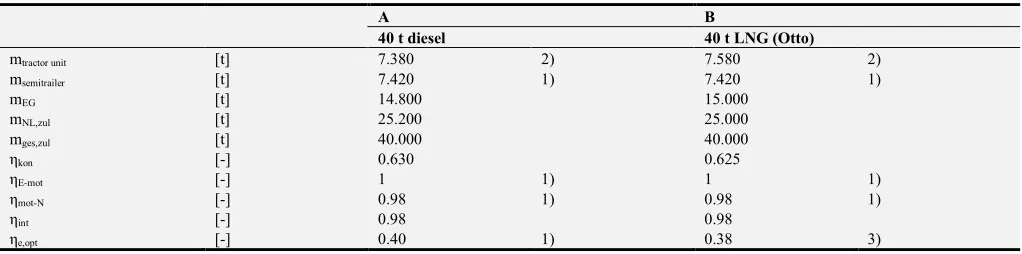
Table 3. Vehicle efficiency comparison 40 tonner Stralis NP 400 with ηe,opt = 0.38 v. Stralis XP 420 (Dies.).

A B

40 t diesel 40 t LNG (Otto)

mtractor unit [t] 7.380 2) 7.580 2)

msemitrailer [t] 7.420 1) 7.420 1)

mEG [t] 14.800 15.000

mNL,zul [t] 25.200 25.000

mges,zul [t] 40.000 40.000

ηkon [-] 0.630 0.625

ηE-mot [-] 1 1) 1 1)

ηmot-N [-] 0.98 1) 0.98 1)

ηint [-] 0.98 0.98

(6)

A B

ηE-N,opt [-] 0.39 0.37

α1 [-] 1.00 1.00

Fe [-] 4.05 4.30

B/A [-] 1.06

Annotations:

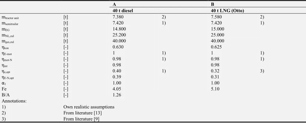
Table 4. Vehicle efficiency comparison 40 tonner Stralis NP 400 with ηe,opt = 0.32 v. Stralis XP 420 (Dies.).

A B

mtractor unit [t] 7.380 2) 7.580 2)

msemitrailer [t] 7.420 1) 7.420 1)

mEG [t] 14.800 15.000

mNL,zul [t] 25.200 25.000

mges,zul [t] 40.000 40.000

ηkon [-] 0.630 0.625

ηE-mot [-] 1 1) 1 1)

ηmot-N [-] 0.98 1) 0.98 1)

ηint [-] 0.98 0.98

ηe,opt [-] 0.40 1) 0.32 3)

ηE-N,opt [-] 0.39 0.31

α1 [-] 1.00 1.00

Fe [-] 4.05 5.10

B/A [-] 1.26

Annotations:

The result of recording the efficiency , of the LNG

engine once with 0.38 = 0.95 · 0.40 and once with 0.32 = 0.80 · 0.40 are Fe coefficients of the LNG traction unit of 4.3 and 5.1 respectively as against a 4.05 Fe coefficient for the diesel-driven counterpart ( , = 0.40). Setting the Fe

coefficients relative to one another results in that - for all instances of α1 = 1 - the consumption of the gas-driven articulated lorry per transported ton and km is approx. 6% or 26% higher than that of the diesel-driven articulated lorry. Cf. Tables 3 and 4! (Note: even when this comparison of the specific final energy demand eE in kWh (tank-to-wheel) is

unfavourable towards the fossil natural gas driven truck (NG), it still does not say anything about its environmental friendliness - in particular on its admixture with biogas. Compare in this respect [9, S. 2-69 – 2-70]).

7. Conclusion, Critical Reflection,

Outlook

As essentially a multitude of parameters (Formula 8) have to be inputted into the energy demand calculation (Chapter 3), comparing different drive chain trucks on their consumption (and environmental compatibility) can be highly complex. The answer is easy when replying to the question which generally satisfies for an initial assessment „To what extent does the fuel consumption per transported ton and km (under full load capacity) change when the drive chain is replaced in a given truck but with

the outer shape and permitted total weight (vehicle parameters) and the deployment conditions (route parameters) remaining the same ?“ In this instance, it suffices to ascertain the vehicle efficiency coefficients Fe

as developed in this article (Chapter 3) for the various drive concepts (Formula 11) and compare them. The lower the Fe, the lower the specific final energy consumption eE

and the higher is the vehicle efficiency in comparison. But any simplification has its drawbacks. This kind of (initial) comparison takes no account of possibly different ranges of the vehicles which, under certain circumstances, necessitate adjustments to the net weight mEG and/or the permitted payload mNL,zul or the possibility of recuperating energy when braking, which, in turn, results in a reduction of the specific consumption eE.

The outcome of Case Study 1 (Chapter 4) concerned with an (initial) comparison of the efficiency of the Fuso eCanter over its diesel-driven counterpart in the shape of the pendant Fuso Fe 160 (both 7.5 tonners) was one of the eCanter requiring approx. 50% less final energy per transported ton and mileage undertaken than the FE 160.

(7)

The outcome of Case Study 3 (Chapter 6) concerned with the efficiency of a gas-driven 40 t articulated lorry over its diesel-driven counterpart is one whereby - conditional upon the efficiency 0.8 ≤ ηe,opt ≤ 0.95 of the gas engine (Otto principle) - the final energy demand per tkm is 6% to 26% higher than for the diesel-driven counterpart.

For simplification purposes, α1 = 1 was assumed for all the three case studies. The risks inherent in the differences

in ranges were knowingly accepted. No consideration was given to the recuperation possibilities of the electric battery vehicles.

This article focussed on a calculation proposal to compare specific final energy demands eE in kWhE/t/km. It

goes without saying it allows deductions to be made as to primary energy demands eP in kWhP/t/km as well as CO2

e-emissions mCO2 in kg/t/km.

Abbreviations

A cross-section area

DÄ diesel equivalent

EE final energy provided

EN useful energy supplied at the wheels

Fmass mass-dependent motion resistance

Faer air resistance

Fe vehicle efficiency coefficient

HPDI High Pressure Direct Injection

I incline

TS Tesla Semi

cW air resistance coefficient

ee specific final energy consumption

ep specific primary energy consumption

el electric

g gravitational acceleration

mtractor unit net mass of tractor unit

msemitrailer net mass of semitrailer

mChassis net mass of chassis

mbox body net mass of box body

mtail lift net mass of tail lift

mEG net mass

mNL payload

mNL,zul permissible payload

mges,zul gross vehicle weight

mCO2 mass of CO2e-emissions

s distance

v speed

α1 drive line factor

α2 route factor

ηe = ηmot motor efficiency

ηe,opt motor efficiency at the ideal operating point

ηE-mot energy efficiency between final energy supply and motor terminal

ηE-N energy efficiency between final energy supply and wheels

ηE-N,opt optimum energy efficiency between final energy supply and wheels

ηint = ηE-mot + ηmot-N

ηkon design efficiency

ηmot =ηe motor efficiency

ηmot-N energy efficiency degree between motor shaft and wheels

µR rolling friction coefficient

(8)

References

[1] N. N.: Klimaschutzplan 2050. Deutsches Bundesministerium für Umwelt, Naturschutz und nukleare Sicherheit (BMU), Arbeitsgruppe IK III 1, Berlin. November 2016. https://www.bmu.de/fileadmin/Daten_BMU/Download_PDF/ Klimaschutz/klimaschutzplan_2050_bf.pdf.

[2] Weiß, Martin; Welke, Mareike: Klimaschutz in Zahlen. Fakten, Trends und Impulse deutscher Klimapolitik. Deutsches Bundesministerium für Umwelt, Naturschutz, Bau und Reaktorsicherheit (BMUB), Referat KI I 1, Berlin. April 2017.

http://www.bmub.bund.de/fileadmin/Daten_BMU/Pools/Brosc hueren/klimaschutz_in_zahlen_2017_bf.pdf.

[3] N. N.: Gerichts-Hammer: Städte dürfen Diesel-Fahrverbote erlassen. Onlineportal Merkur.de, München, 28.02.18.

https://www.merkur.de/politik/hammer-urteil- bundesverwaltungsgerichts-in-leipzig-staedte-duerfen-diesel-fahrverbote-erlassen-zr-9649379.html.

[4] N. N.: Trend guide – Alles was 2018 wichtig ist! ETM-Verlag, Stuttgart, 2018.

[5] Crissey, Jeff: Mitsubishi Fuso delivers first all-electric eCanter trucks to customers. https://www.ccjdigital.com/mitsubishi-fuso-delivers-first-all-electric-ecanter-trucks-to-customers/. Commercial Carrier Journal. Posted on 14.09.2017.

[6] Gross, L. J.: Analysis: The Tesla semi’s major selling points. https://www.joc.com/technology/analysis-telsa-semis-major-selling-points_20171228.html. joc.com. Posted on 28.12.2017.

[7] Hoffmann, J.: Scania zieht nach – Schwedischer Lkw-Hersteller setzt zunehmend auf Erdgas. transaktuell 5. ETM-Verlag, Stuttgart, 15.2.2018.

[8] Schmidt, B.: Iveco und Scania geben Gas. Onlineportal Frankfurter Allgemeine faz.net, Frankfurt, 03.12.2017. http://www.faz.net/aktuell/technik-motor/motor/lastwagen-mit-lng-iveco-und-scania-geben-gas-15311802-p2.html. [9] Bünger, U. et alt.: Vergleich von CNG und LNG zum Einsatz

in Lkw im Fernverkehr. Abschlussbericht. Ludwig-Bölkow- Systemtechnik GmbH, Ottobrunn, Mai 2016. http://www.lbst.de/ressources/docs2016/1605_CNG_LNG_En dbericht_public.pdf.

[10] Franke, K.-P.: Raising the efficiency of Long Distance Road Haulage by Introducing Extra Long Trucks. Proceedings of the VII International Scientific Conference “Logistic Systems in Global Economics”, S. 21 -29. Krasnoyarsk 2017. http://vseup.ru/static/files/2017.pdf.

[11] Haag, M.; Künzel, T.: Plausibilisierung eines Rechenmodells für Fernverkehrs-Lkw. Master-Projektarbeit an der Hochschule Ulm. 03.2018 (not published).

[12] N. N.: Fuso Ecanter. WIKIPEDIA.

https://de.wikipedia.org/wiki/Fuso_Ecanter. (Download 8.3.2018).

[13] Burgdorf, J.: Supertest Iveco Stralis NP 400: Spass mit dem Gas? Trucker.de –Test & Technik –Tests. Springer Fachmedien München GmbH, München, 10.01.2018. http://www.trucker.de/supertest-iveco-stralis-np-400-spass-mit-dem-gas-2036790.html.

[14] N. N.: Sattelzugmaschine Scania LNG – Flüssiges ERDGAS für Langstreckenstars. Zukunft ERDGAS GmbH, Berlin.

https://www.erdgas.info/erdgas-mobil/erdgas-fahrzeuge/scania/scania-pg-lng-340/. (Download 26.04.2019). [15] Linde: LNG (Erdgas flüssig). Produktdatenblatt, Stand

21.04.2008. https://produkte.linde-gase.de/db_neu/lng_erdgas_fluessig.pdf.

[16] Wurster, R. et alt.: LNG als Alternativkraftstoff für den Antrieb von Schiffen und schweren Nutzfahrzeugen, S. 95. Kurzstudie im Auftrag des Deutschen Bundesverkehrsministeriums für Verkehr und digitale Infrastruktur (BMVI). Deutsches Zentrum für Luft- und Raumfahrt e. V. (DLR), Institut für Verkehrsforschung; ifeu – Institut für Energie- und Umweltforschung Heidelberg GmbH; Ludwig-Bölkow-Systemtechnik GmbH (LBST); Deutsches Biomasseforschungszentrum gGmbH (DBFZ); München/Ottobrunn, Heidelberg, Leipzig, Berlin, 06.03.2014.

http://biogasrat.de/wp-content/uploads/2018/01/mks-kurzstudie-lng.pdf.

[17] Prenzler, Christian: Tesla Semi unveiled: 500+ range, Bugatti-beating aero, 2019 production.

https://www.teslarati.com/tesla-semi-unveiled-coming-2019-500-mile-range/. Teslarati. Posted on 16.11.2017.

[18] Rosenberger, T.: Keine Kompromisse. trans aktuell 24. ETM Verlag, Stuttgart.1.12.2017.