R E S E A R C H
Open Access
Directional global three-part image
decomposition
D. H. Thai
1,2*and C. Gottschlich
1Abstract
We consider the task of image decomposition, and we introduce a new model coined directional global three-part decomposition (DG3PD) for solving it. As key ingredients of the DG3PD model, we introduce a discrete
multi-directional total variation norm and a discrete multi-directional G-norm. Using these novel norms, the proposed discrete DG3PD model can decompose an image into two or three parts. Existing models for image decomposition by Vese and Osher (J. Sci. Comput. 19(1–3):553–572, 2003), by Aujol and Chambolle (Int. J. Comput. Vis. 63(1):85–104, 2005), by Starck et al. (IEEE Trans. Image Process. 14(10):1570–1582, 2005), and by Thai and Gottschlich are included as special cases in the new model. Decomposition of an image by DG3PD results in a cartoon image, a texture image, and a residual image. Advantages of the DG3PD model over existing ones lie in the properties enforced on the cartoon and texture images. The geometric objects in the cartoon image have a very smooth surface and sharp edges. The texture image yields oscillating patterns on a defined scale which are both smooth and sparse. Moreover, the DG3PD method achieves the goal of perfect reconstruction by summation of all components better than the other considered methods. Relevant applications of DG3PD are a novel way of image compression as well as feature extraction for applications such as latent fingerprint processing and optical character recognition.
Keywords: Image decomposition, Variational calculus, Cartoon image, Texture image, Image compression, Feature extraction, Latent fingerprint image processing, Optical character recognition, Fingerprint recognition
1 Introduction
Feature extraction, denoising, and image compression are key issues in computer vision and image processing. We address these main tasks based on the paradigm that an image can be regarded as the addition or montage of several meaningful components. Image decomposi-tion methods attempt to model these components by their properties and to recover the individual components using an algorithm. Relevant component images include geometrical objects which have piece-wise constant val-ues or a smooth surface like the characters in Fig. 1b or components which are filled with an oscillating pattern like the fingerprint in Fig. 1c.
Based on these observations, we define the following goals:
*Correspondence: [email protected]
1Institute for Mathematical Stochastics, University of Goettingen, Goldschmidtstr. 7, 37077 Goettingen, Germany
Full list of author information is available at the end of the article
Goal 1: the cartoon componentucontains only geometri-cal objects with a very smooth surface, sharp boundaries, and no texture.
Goal 2: the texture component vcontains only geomet-rical objects with oscillating patterns andvshall be both smooth and sparse.
Goal 2: three-part decomposition and reconstructionf= u+v+.
How does achieving these goals serve the tasks of fea-ture extraction, denoising, and compression?
Extremely efficient representations of the cartoon image uand texture imagevexist. These two component images are highly compressible as discussed with full details in Section 7.3. Depending on the application, u or v or both can be considered as feature images. For the appli-cation to latent fingerprints, we are especially interested in the texture image v as a feature for fingerprint seg-mentation and all subsequent processing steps. Example results for the very challenging task of latent finger-print segmentation are given in Section 7.1. In optical character recognition (OCR), pre-processing includes the
Fig. 1The simulated latent fingerprint (a) is composed by adding the fingerprint (c) to image (b) which is a detail from a photo of a printed document. DG3PD decomposition ofaobtains a smooth cartoon image u (d) and a smooth and sparse texture image v (e). All positive coefficients of v are visualized as white pixels inf. The region of interest shown ingis estimated from vbinusing morphological operations [57]. Imageiis
composed frombandhand decomposed by DG3PD into cartoon (j), texture (k), and residual (l)
removal of complex background and the isolation of char-acters. After three-part decomposition and depending on the scale of the characters, the cartoon image u con-tains the information of interest for OCR (see Fig. 1j), and the background is separated intovand simultane-ously in the minimization procedure. As a consequence of the requirements imposed on u and v, noise and small scale objects are driven into the residual image
during the decomposition of f. Therefore, the image u + v can be regarded as a denoised version of f and the degree of denoising can be steered by the choice of parameters.
The paper is organized as follows. In Section 2, we begin by describing notation and preliminaries. After hav-ing established these prerequisites, we define the DG3PD model in Section 3 and in Section 4; we explain its relation to existing models in the literature for two-part and three-two-part decomposition. In Section 5, we describe an iterative, numerical algorithm which solves the DG3PD model for practical applications to dis-crete, two-dimensional images. In Section 6, we per-form a detailed comparison of the DG3PD method to state-of-the-art decomposition approaches. Applications of DG3PD, especially feature extraction and image com-pression, are the topics in Section 7. Discussion and conclusions are given in Section 8. An overview of the algorithm and an additional comparison is given in the Appendix.
2 Notation and preliminaries
For simplification, we use a bold symbol to denote the coordinates of a two-dimensional signal, e.g., x = (x1,x2),k =[k1,k2] ,ω = (ω1,ω2), and ejω =
ejω1,ejω2. A two-dimensional imagef[k] :→R+, the
discretization of the continuous version f(x) (i.e.f[k]= f(x)|x=k∈), is specified on the lattice:
=(k1,k2)∈[ 0 ,m−1]×[ 0 ,n−1]⊂N20
.
LetXbe the Euclidean space whose dimension is given by the size of the lattice, i.e.,X=R||. The 2D discrete Fourier transformFacting onf[k] is
f[k] ←→F F(ejω)=
k∈
f[k]·e−jk,ω2,
whereωis defined on the lattice:
I=
(ω1,ω2)=
2πn n ,
2πm m |(n
,m)∈−n
2, n 2
× −m
2 , m
2
⊂Z2,
i.e.,ω∈[−π,π]2.
Forward and backward difference operators:Given the matrix
Dm=
⎛ ⎜ ⎜ ⎜ ⎜ ⎜ ⎝
−1 1 0 . . . 0 0 −1 1. . . 0
..
. ... ... . .. ... 0 0 0 . . . 1 1 0 0 . . . −1
⎞ ⎟ ⎟ ⎟ ⎟ ⎟ ⎠∈R
m×m,
the forward and backward difference operators with peri-odic boundary condition in convolution and matrix forms and their Fourier transform are explained in Table 1.
Discrete directional derivative: Let ∇+ =
∂+ x ,∂y+
be the discrete forward gradient operator with ∂x+ and ∂+
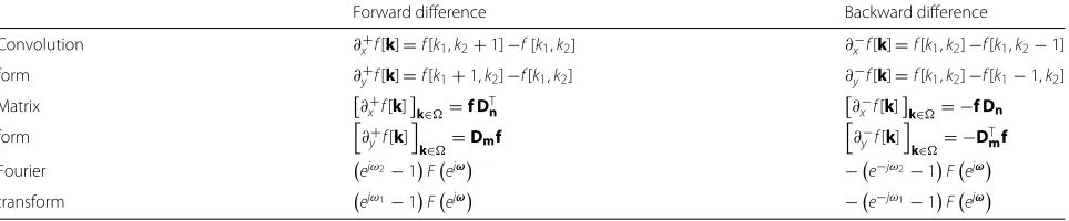
Table 1Forward/backward difference with periodic boundary condition in convolution/matrix form and their Fourier transform
Forward difference Backward difference
Convolution ∂x+f[k]=f[k1,k2+1]−f[k1,k2] ∂x−f[k]=f[k1,k2]−f[k1,k2−1]
form ∂y+f[k]=f[k1+1,k2]−f[k1,k2] ∂y−f[k]=f[k1,k2]−f[k1−1,k2]
Matrix ∂x+f[k]k∈=f DnT ∂x−f[k]k∈= −f Dn
form ∂y+f[k]
k∈=Dmf
∂−
yf[k]
k∈= −D T mf
Fourier ejω2−1Fejω −e−jω2−1Fejω
transform ejω1−1Fejω −e−jω1−1Fejω
DT
nandDTmare the transposed matrices ofDnandDm, respectively
following the direction−→d =
cosπLl, sinπLl T
withl = 0 ,. . .,L−1 is defined as
∂l+=−→d ,∇+ =cos π l L ∂ + x + sin
π l L ∂
+ y.
Thus, the discrete directional gradient operator is
∇L+=∂l+l∈[0,L−1]. (1)
2.1 Discrete directional TV norm
The continuous total variation norm has been defined in [1]. Due to the discrete nature of images, we define its discrete version with forward difference operators as
∇+u
1 =
k∈
∂x+u[k] 2
+∂y+u[k] 2
.
We extend it into multi-direction L with the discrete directional gradient operator (1):
∇+ Lu1 =
k∈
L−1
l=0
∂l+u[k]2
= L−1
l=0
cosπl LuD
T
n+sin
πl LDmu
2
1
.
The discrete anisotropic total variation norm in a matrix form is
∇+ Lu1 =
L−1
l=0 cosπl
LuD
T
n+sin
πl L Dmu
1
. (2)
2.2 Discrete directional G-norm
Discrete G-norm: Meyer [2] has proposed a space G of continuous functions to measure oscillating functions (texture and noise). The discrete version of the G-norm has been introduced by Aujol and Chambolle in [3]. We rewrite it with the matrix form of the forward difference operators as
vG=inf
g21+g22
∞,v=g1D
T n+Dmg2,
gl
l∈[1,2]∈X 2
.
(3)
Discrete directional G-norm: We extend (3) into multi-directionsS∈N+with the directional difference operator to obtain the discrete directional G-norm as
vGS=inf
⎧ ⎪ ⎪ ⎪ ⎪ ⎪ ⎪ ⎪ ⎪ ⎪ ⎨ ⎪ ⎪ ⎪ ⎪ ⎪ ⎪ ⎪ ⎪ ⎪ ⎩ S−1
s=0 g2 s ∞ , v=
S−1
s=0
cosπs S gsD
T n+sin
πs S Dmgs
# $% &
⇔v[k]=S'−1 s=0
∂s+gs[k] ,∀k∈ ,
gs
S−1
s=0 ∈X
S ⎫ ⎪ ⎪ ⎪ ⎪ ⎪ ⎪ ⎪ ⎪ ⎪ ⎬ ⎪ ⎪ ⎪ ⎪ ⎪ ⎪ ⎪ ⎪ ⎪ ⎭ . (4) 3 DG3PD
We define the DG3PD model for discrete directional three-part decomposition of an image into cartoon, tex-ture, and residual parts as
min (u,v,)∈X3
∇L+u1+μ1vGS+μ2v1
s.t. sup (i,l,k)∈K
++Ci,l{}[k]++≤δ, f=u+v+
,
(5)
where C is the curvelet transform [4, 5] with the index set K. Please note that by setting the parameter δ = 0 in (5), we obtain a two-part decomposition which can be considered as a special case of the DG3PD model. Next, we discuss how the DG3PD model relates to existing decomposition models.
4 Related work
Mumford and Shah: In 1989, Mumford and Shah [6] have proposed piecewise smooth (for image restoration) and piecewise constant (for image segmentation) models by minimizing the energy functional. This approach can be considered as a precursor for subsequent image decomposition models with texture components. How-ever, due to the Hausdorff one-dimensional measureH1 inR2, it poses a challenging or even NP-hard problem in optimization to minimize the Mumford and Shah func-tional. Later, based on the Mumford and Shah model, Chan and Vese [7] have proposed an active contour for image segmentation which they solved by a level set method [8].
Rudin, Osher, and Fatemi: In 1992, Rudin et al. [1] pio-neered image decomposition with a two-part model for denoising.
Meyer: The model defined by Meyer in 2001 [2] for a two-part decomposition in the continuous setting is com-prised in the DG3PD model for the special case ofL = S=2 andμ2=δ=0 in the discrete domain.
Vese and Osher: In 2003, Vese and Osher [9] solved Meyer’s model for two-part decomposition in the con-tinuous setting and they proposed to approximate the L∞-norm in the G-norm by theL1-norm and to apply the
penalty method for reformulating the constraint. For prac-tical application to images, they discretized their solution. This approach is extended in [10].
Aujol and Chambolle: Aujol and Chambolle in 2005 [3] adapted the work by Meyer for discrete two-part decom-position (see (5.49) in [3]), and they used the penalty method for the constraint. Their model is included in the DG3PD model with parametersL=S=2,μ1= μ2=0
and applying the supremum norm to the wavelet coeffi-cients of the oscillating pattern, i.e.,W{·}∞, instead of the curvelet coefficientsC{·}∞as in the DG3PD model. Moreover, Aujol and Chambolle proposed a model for dis-crete three-part decomposition (see (6.59) in [3]) which measures texture by the G-norm and noise by the supre-mum norm of wavelet coefficients and the penalty method for the constraint. Different from Vese and Osher as well as our approach explained later, they describe the G-norm for capturing texture using the indicator function defined on a convex set and they obtain the solution by Cham-bolle’s projection onto this convex set. Their model is included in the DG3PD model for parametersL=S=2, μ2 = 0 and using wavelets instead of curvelets for the
residual as before.
Starck et al.: Starck et al. [11] introduced a model for two-part decomposition based on a dictionary approach. Their basic idea is to choose one appropriate dictio-nary for piecewise smooth objects (cartoon) and another suitable dictionary for capturing texture parts.
Aujol et al.: In 2006, Aujol et al. [12] proposed a two-part decomposition of an image into a structure component
and a texture component using Gabor functions for the texture part.
Gilles: Gilles [13] proposed a three-part image decom-position method in 2007 which is similar to the Aujol-Chambolle model [3], but G-norm is used as a measure-ment of the residual (or noise) instead of Besov space
˙
B∞−1,∞with a local adaptability property. Their argument is that the more a function is oscillatory, the smaller is the G norm. Then, they propose a new “merged-algorithm” with a combination of a local adaptivity behavior and Besov space.
Maragos and Evangelopoulos: In 2007, Maragos and Evangelopoulos [14] have proposed a two-part decompo-sition model which relies on energy responses of a bank of 2D Gabor filters for measuring the texture component. They discuss the connection between Meyer’s oscillat-ing functions [2], Gabor filters [15], and AM-FM image modeling [16, 17].
Buades et al.: In 2010, Buades et al. [18] derived a non-linear filter pair for two-part decomposition into cartoon and texture parts. Further models for two-part decompo-sition are listed in Table 1 of [18].
Maurel et al. and Chikkerur et al.: In 2011, Maurel et al. [19] proposed a decomposition approach which models the texture component by local Fourier atoms. For finger-print textures, Chikkerur et al. [20] proposed in 2007 the application of local Fourier analysis (or short-time Fourier transform, STFT) for image enhancement. However, the usefulness of local Fourier analysis for capturing texture information depends on and is limited by the level of noise in the corresponding local window, see Figure 2c in [21] for an example in which STFT enhances some regions successfully and fails in other regions.
Ono et al.: In 2014, Ono et al. [22] proposed a cartoon-texture decomposition using the block nuclear norm (an generalized version of [23]) which interprets the texture component as the combination of overlapped and sheared blockwise low-rank matrices in different directions. The underlying assumption is that “texture, in general, is glob-ally dissimilar but locglob-ally well patterned.” Similar to our directional G-norm, the shear helps to handle patterns in non-horizontal or vertical. However, their cartoon com-ponent still contains some texture and their texture is not highly sparse, i.e., the non-zero coefficients are only due to texture component, see Fig. 4a and d, respectively. More-over, they use 1 or 2 norm for the data-fidelity term.
However, according to [2, 24], “oscillatory components do not have small norms in L2() or L1().” In our case,
we use the Banach C{·} which is more suitable than the Banach space E = B−∞1,∞ in equation (1.3) [3] for measuring small-scale objects, e.g., noise.
texture imagevwhich serves as a useful feature for esti-mating the region of interest (ROI). The G3PD model is included in the DG3PD model by choosing L = 2 and replacing the directional G-norm in the DG3PD model by the1-norm of curvelet coefficients (multi-scale
and multi-orientation decomposition) to capture texture. However, a disadvantage of the1-norm of curvelet
coef-ficients is a tendency to generate the halo effect on the boundary of the texture region due to the scaling factor in curvelet decomposition (see Figure 3d in [25]), whereas the directional G-norm in the DG3PD model is capable to capture oscillating patterns (see [2]) without the halo effect.
Directional total variation and G-norm:In Section 2.1, we introduced the discrete directional total variation norm, and in Section 2.2, we introduced the discrete direc-tional G-norm. Please note the aspect of summation over multiple directions in Eqs. (2) and (4).
The term “directional total variation” has previously been used by Bayram and Kamasak [26, 27] for defining and computing the TV norm in only one specific direc-tion. They have treated the special case of images with one globally dominant direction and addressed those by two-part decomposition and for the purpose denoising. Zhang and Wang [28] proposed an extension of the work by Bayram and Kamasak for denoising images with more than one dominant direction.
5 Solution of the DG3PD model
Now, we present a numerical algorithm for obtaining the solution of the DG3PD model stated in (5). Givenδ >0, denote G∗δ as the indicator function on the feasible convex setA(δ)of (5), i.e.,
A(δ)=∈X : C{}∞ ≤δ andG∗, δ
=
0 , ∈A(δ)
+∞, ∈/A(δ) .
By analogy with the work of Vese and Osher, we con-sider the approximation of G-norm with 1 norm and
the anisotropic version of directional total variation norm. The minimization problem in (5) is rewritten as
To simplify the calculation, we introduce two new variables:
rb=cos ,
πb L
uDTn+sin
, πb
L
Dmu, b=0 ,. . .,L−1,
wa=ga,a=0 ,. . .,S−1 .
Equation (6) is a constrained minimization problem. The augmented Lagrangian method (ALM) is applied to turn (6) into an unconstrained one as
min
,
u,v,,[rl]lL=−01,[ws]Ss=−01,[gs]Ss=−01
∈XL+2S+3L
,
u,v,, [rl]Ll=−01,
[ws]Ss=−01 ,
gs S−1
s=0 ; [λ1l] L−1
l=0 , [λ2s]Ss=−01,λ3,λ4
,
(7)
where the Lagrange function is
L(·;·)=
L−1
l=0
rl1+μ1
S−1
s=0
ws1+μ2v1+G
∗, δ
+β1
2
L−1
l=0 rl−cos
πl
L uD
T n−sin
πl
L Dmu
λ1l
β1 2
2
+β2
2
S−1
s=0
ws−gs+λ2s
β2 2
2
+β3
2 v−
S−1
s=0
cos ,πs
S
gsDTn+sin ,πs
S
Dmgs
+λ3 β3 2 2
+β4
2
f−u−v−+λ4
β4 2
2
.
Due to the minimization problem with multi-variables, we apply the alternating directional method of multipli-ers to solve (7). Its minimizer is numerically computed through iterationst=1 , 2 ,. . .
u(t),v(t),(t),r(lt) L−1
l=0 ,
w(st) S−1
s=0 ,
g(st) S−1
s=0 =
arg minL,u,v,, [rl]Ll=−01, [ws]Ss=−01,
gs S−1
s=0 ;
λ(t−1) 1l
L−1
l=0 ,
λ(t−1) 2s
S−1
s=0 ,λ
(t−1)
3 ,λ
(t−1) 4
(8)
and the Lagrange multipliers are updated after every step t with a rate γ. We initializeu(0) = f,v(0) = (0) =
r(l0) L−1
l=0 =
w(s0) S−1
s=0 =
g(s0) S−1
s=0 =
λ(0) 1l
L−1
l=0 =
,
u∗,v∗,∗,gs∗Ss=−01=, arg min
u,v,,[gs]Ss=−01
∈XS+3
L−1
l=0 cos π l L uD T
n+sin
π l L Dmu
1
+μ1 S−1
s=0
gs1+μ2v1+G ∗, δ s.t. ⎧ ⎨ ⎩
f=u+v+
v=S'−1 s=0
cosπSsgsDTn+sin
πs S
Dmgs
⎫ ⎬ ⎭.
λ(0)
2a S−1
a=0 = λ
(0)
3 = λ
(0)
4 = 0. In each iteration, we first
solve the following six subproblems in the listed order and then we update the four Lagrange multipliers:
The “[rl]Ll=−01-problem”: Fixu,v,, [ws]Ss=−01,
gs S−1
s=0and
min
[rl]Ll=−01∈X
L L−1
l=0
rl1+
β1
2 L−1
l=0 rl−cos
π l L uD T n −sin π l
L Dmu+
λ1l β1 2 2 (9)
Due to its separability, we consider the problem at b=0 ,. . .,L−1. The solution of (9) is
r∗b = Shrink cos πb L uD T n+sin
πb
L Dmu−
λ1b
β1 , 1
β1 .
The operator Shrink(·,·)is defined in [25]. The “[ws]Ss=−01-problem”: Fixu,v,, [rl]Ll=−01,
gs
S−1 s=0 and
min
[ws]Ss=−01∈XS
μ1
S−1
s=0
ws1+
β2
2 S−1
s=0
ws−gs+λβ2s 2 2 2 (10)
Similarly, the solution of (10) for each separable problem a=0 ,. . .,S−1 is
w∗a = Shrink ⎛ ⎜ ⎜ ⎜
⎝ga−λβ2a 2 # $% &
:=twa ,μ1
β2 ⎞ ⎟ ⎟ ⎟
⎠. (11)
The “[gs]Ss=−01-problem”: Fixu,v,, [rl]lL=−01, [ws]Ss=−01and
min [gs]Ss=−01∈XS
β2
2
S−1
s=0
ws−gs+λ2s
β2 2
2
+β3
2 v−
S−1
s=0
cos,πs S
gsDTn
+sin,πs S
Dmgs
+λ3β
3 2 2 (12)
For the discrete finite frequency coordinates ω = [ω1,ω2]∈ I, let be z =[z1,z2]=
ejω1,ejω2. We
denote byWa(z),2a(z),V(z),Gs(z), and3(z)the
dis-crete Fourier transforms ofwa[k] ,λ2a[k] ,v[k] ,gs[k] and λ3[k], respectively. Due to the separability, the solution of
(12) is obtained fora=0 ,. . .,S−1 as
g∗a = ReF−1{A(z)·B(z)} (13) with
A(z)=
-β2+β3
sinπa S
,
z−11−1
+cosπa S
,
z−21−1
sinπa
S (z1−1)+cos
πa S (z2−1)
−1 ,
B(z)=β2 .
Wa(z)+2a(
z) β2
/
+β3
sin ,πa
S ,
z−11−1
+cos,πa S
(z−21−1)× ⎡
⎣V(z)−
s=[0 ,S−1]\{a}
cos
,πs S
(z2−1)+sin ,πs
S
(z1−1)
Gs(z)+3(
z) β3
⎤ ⎦.
The “v-problem”: Fixu,, [rl]Ll=−01, [ws]Ss=−01,
gs S−1
s=0and
min
v∈X
μ2v1+β3 2
v−
4S−1
s=0
cos ,πs
S
gsDTn
+ sin,πs S
Dmgs
− λ3
β3 2
2 +β4
2 v−
f−u−+λ4 β4
2
2
(14)
The solution of (14) is defined as
v∗ = Shrink
tv, μ2
β3+β4
, (15)
with
tv := β3
β3+β4 4S−1
s=0
cos,πs S
gsDTn+sin,πs S
Dmgs
−λ3
β3 5
+ β4
β3+β4
f−u−+λ4 β4 .
(16)
The “u-problem”: Fixv,, [rl]Ll=−01, [ws]Ss=−01,
gs S−1
s=0and
min u∈X
β1 2
L−1
l=0 rl−cos
π l
L uD
T n−sin
π l
L Dmu+
λ1l
β1 2
2
+ β4 2
f−u−v−+λ4 β4 2 2 (17)
We denote F(z),E(z),4(z),Rl(z), and1l(z) as the discrete Fourier transforms of f[k] ,[k] ,λ4[k] ,rl[k], andλ1l[k], respectively. This (17) is solved in the Fourier domain by
with
X(z)=
-β4+β1 L−1
l=0 . sin πl L , z−11−1
+cos πl L ,
z−21−1
/ . sin
πl
L (z1−1)+cos
πl
L (z2−1) /6−1
,
Y(z)=β4 .
F(z)−V(z)−E(z)+4(z) β4
/ +β1
L−1
l=0 . sin π l L , z−11−1
+cos π l L , z−21−1
/ .
Rl(z)+1l( z) β1
/ .
The “-problem”: Fixu,v, [rl]lL=−01, [ws]Ss=−01,
gs S−1
s=0, and
min ∈X G∗ , δ
+β4
2 −
f−u−v+ λ4 β4
2
2
(19)
LetC∗ be the inverse curvelet transform [4]. The mini-mization of (19) is solved by (see [3])
∗=f−u−v+ λ4
β4
−C∗ShrinkCf−u−v+λ4
β4 7
,δ 7
# $% &
:=CST
,
f−u−v+λ4 β4,δ
or by the projection method with the component-wise operators
∗=C∗
⎧ ⎨ ⎩
δC8f−u−v+ λ4
β4
max,δ, +++C8f−u−v+ λ4
β4
+++ ⎫ ⎬ ⎭.
Update Lagrange multipliers ,
[λ1l]Ll=−01, [λ2a]Sa−=10, λ3,λ4)∈XL+S+2:
λ(t)
1b=λ (t−1)
1b + γβ1
rb−cos
πb L uD T n −sin πb
L Dmu , b=0 ,. . .,L−1
λ(t)
2a=λ( t−1)
2a +γβ2(wa−ga), a=0 ,. . .,S−1
λ(t)
3 =λ(
t−1)
3 +γβ3
4 v−
S−1
s=0
cos,πs S
gsDTn
+ sin,πs S
Dmgs
5
λ(t)
4 =λ(
t−1)
4 +γβ4(f−u−v−)
Choice of parameters
Due to the1-norms in the minimization problem (7)
which corresponds to the shrinkage operator with param-etersμ1andμ2, these are defined as
μ1 = cμ1β2·maxk∈++twa[k]++ and
μ2 = cμ2(β3+β4)·maxk∈(|tv[k]|), (20)
wheretwa[k] andtv[k] are defined in (11) and (16), respec-tively. Note that the choice ofcμ1 andcμ2 is adapted to
specific images.
In order to balance between the smoothing terms and the updated terms for the solutions of theg-problem in (13), thev-problem in (15), and theu-problem in (18), we choose
β2=c2β3,β3= θ
1−θβ4,θ ∈(0, 1)andβ1=c1β4.
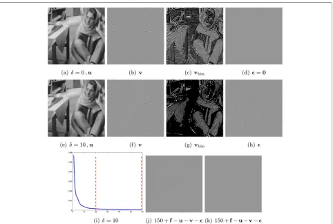
The choice of δ mainly impacts the smoothness and sparsity of the texturev. The first row of Fig. 2 shows the effect of selecting the thresholdδ=0 which corresponds to a two-part decomposition, i.e., the residual image=0 in (d). This case also demonstrates the limitation of all two-part decomposition approaches: for this choice ofδ, very small scale objects are assigned to the texture imagev in Fig. 2b which is obvious in its binarizationvbinshown in
(c). In order to remove these and to yield a smoother and sparser texturev, one can increase the value ofδ, say, e.g., by choosingδ=10. The effect of this choice can be seen in the binarized versionvbinin Fig. 2g and small-scale objects
are moved to the residual image in (h). Therefore, the value ofδdefines the level of the residual.
6 Comparison of DG3PD with prior art
As stated before, the main objective of the DG3PD model is to achieve the following three goals (see Section 1):
• Goal 1:ucontains only geometrical objects with a very smooth surface, sharp boundaries, and no texture.
• Goal 2:vcontains only objects with sparse oscillating patterns andvshall be both smooth and sparse.
Fig. 2Visualization of the decomposition results by DG3PD withδ=0 (a–d) andδ=10 (e–h) after 20 iterations. The convergence rates for these decompositions withδ=0 andδ=10 are depicted in Fig. 6m,i, respectively, which plots the relative error (y-axis) as defined in [25] versus the number of iterations (x-axis). The parameters areβ4=0.04 ,θ=0.9 ,c1=1 ,c2=1.3 ,cμ1=cμ2=0.03 ,γ=1 , andS=L=9. Error images are
illustrated injafter 20 iterations and inkafter 60 iterations withδ=10
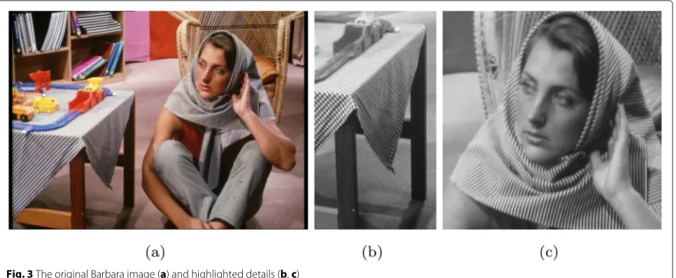
Based on these criteria, we compare the proposed DG3PD model in this section with the state-of-the-art methods using the original Barbara image. We high-light selected regions for an improved conspicuous-ness of the differences between the considered methods; see Fig. 3:
• Images without noise: Rudin, Osher, and Fatemi (ROF) [1], Vese and Osher (VO) [9], Starck, Elad, and Donoho (SED) [11], and TV Gabor (TVG) by Aujol et al. [12] models.
• Images corrupted by i.i.d. Gaussian noiseN(0 ,σ): the Aujol and Chambolle (AC) model [3].
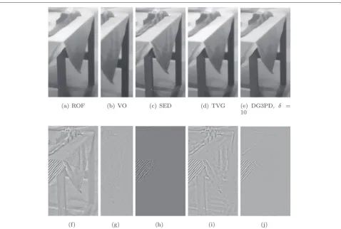
For better visibility of differences between the various models, we show decomposition results for the ROF, VO, SED, TVG, and DG3PD models for two magnified parts of the original image (see Fig. 3b, c) in Figs. 4 and 5. We observe two main differences between the compared models and the proposed DG3PD model:
• Two-part decomposition instead of three-part decomposition.
• Quadratic penalty method (QPM) for solving the constrained minimization instead of ALM.
Fig. 3The original Barbara image (a) and highlighted details (b,c)
Goal 2: texturev.Concerning the texturev, among the state-of-the-art methods, the decomposition by the SED model results in the sparsest texture (see Figs. 4g and 5h), while the texture images of the ROF, VO, and TVG have more coefficients different from zero. In addition, the texture component obtained by the ROF model also con-tains some geometry information which should have been assigned to the cartoon component, see Figs. 4e and 5f. The DG3PD model yields an even sparser texture than the SED model due to thev1 in the minimization (5), see the binarized versions with threshold “0” for visualization in Fig. 4o or Fig. 2g.
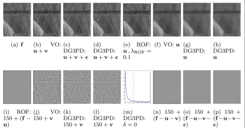
Goal 3: reconstruction by summation of all components. Figures 6 and 7 illustrate the effects of QPM and ALM. The decomposition by the ROF model results in a rela-tively large error (f−u) which contains geometry and texture information; see [9] and Fig. 6i. In the VO model, the error(f−u−v)is reduced in comparison to the ROF model, but some information still remains in the error image; see Fig. 6n. In case of the DG3PD model with the ALM-based approach for solving the constrained mini-mization, the error(f−u−v−)is significantly reduced and numerically the error tends to0as the number of iter-ations increases. For a comparison to ROF and VO using the same detail, see Fig. 6o for a visualization of the error after 20 iterations and (p) after 60 iterations. The error for the whole image after 20 and 60 iterations is displayed in Fig. 2j, k, respectively. To the best of our knowledge, this effect can be explained by using ALM for solving the con-strained minimization instead of QPM. For more details about QPM and ALM, we refer the reader to [29, 30] and Chapter 3 in [31].
Comparison with Aujol and Chambolle.Figure 8 illus-trates a situation in which the image is corrupted by
i.i.d. Gaussian noise N(0 ,σ) with σ = 20 and com-pares DG3PD with the AC model [3] for three-part decomposition. It shows that under “heavy” noise, our DG3PD model still meets the criteria for cartoonuand texturev, i.e.,
• Our cartoonucontains smooth surfaces with sharp edges and no texture; see Fig. 8e. However, the cartoonufrom the AC model is blurry with texture on the scarf; see Fig. 8a.
• Our texturevis sparse and smooth; see Fig. 8f and its binarization (h). However, the texture from the AC model is not sparse; see Fig. 8b.
However, there is a limitation for both methods: the noise image contains some pieces of information due to the value ofδwhich defines the level of the noise. Similar to [3], we modify the classical threshold for curvelet coef-ficients, i.e.,σ92 log|K|, with a weighting parameter η as followsδ = ησ92 log|K| and|K|is total number of curvelet coefficients.
Summary.We observe that the DG3PD method meets all three requirements much more closely than the other methods for images without noise, like the orig-inal Barbara image. And in particular, for images with additive noise, the DG3PD method still achieves all three goals as shown in the comparison with Aujol and Chambolle.
7 Applications
Fig. 4 a–pTheimagesin thefirst rowdepict the comparison of the cartoon u for different methods in the literature on the original highlighted region (see Fig. 3c). Theimagesin thesecond rowshow their corresponding texture v. Note that the ROF is reported in [12]. Theimagesin thethird roware obtained by the DG3PD model withδ=0 andδ=10 in thefourth row(see Fig. 2 for the whole image in these two cases)
7.1 Feature extraction
Depending on the specific field of application, the cartoon or texture, or both can be viewed as feature images. For the application of DG3PD to fingerprints, we are espe-cially interested in the texture image v as a feature for subsequent processing steps like segmentation, orienta-tion field estimaorienta-tion [32] and ridge frequency estimaorienta-tion [15], and fingerprint image enhancement [15, 21]. The first of these processing steps is to separate the foreground from the background [25, 57]. The foreground area (or region of interest) contains the relevant information for a fingerprint comparison. Segmentation is still a challeng-ing problem for latent fchalleng-ingerprints [33] which are very low-quality fingerprints lifted from crime scenes. Both the foreground and background area can contain “noise” on all scales, from small objects or dirt on the surface
to written or printed characters (on paper) and large-scale objects like an arc drawn by the forensic examiner. Standard fingerprint segmentation methods cannot cope with this variety of noise, whereas the texture image by decomposition with the DG3PD method crops out to be an excellent feature for estimating the region of interest. Figure 9 depicts a detailed example of the latent fin-gerprint segmentation by the DG3PD decomposition. In Fig. 10, we show further examples of segmentation results obtained using the texture image extracted by the DG3PD method and morphological postprocessing as described in [25, 57].
7.2 Denoising
Fig. 5 a–jTheimagesin thefirst rowdepict the comparison of the cartoon u for different methods on the originalhighlighted region(see Fig. 3(b)). Theimagesin thesecond rowshow their corresponding texture v
moved into the residual imageduring the decomposition of f due to the supremum norm of the curvelet coeffi-cients of. Therefore, the image fdenoised = u+ vcan
be regarded as a denoised version of f and the degree of denoising can be steered by the choice of parameters, especially δ. For δ = 0 which is equal to two-part decomposition, we obtain the original image again. As we increase δ, more noise is driven into and thereby removed from fdenoised. Denoising images with texture,
in particular with texture parts on different scales, is a relevant problem which we plan to address in future works.
Jung and Kang [34] proposed a variational minimiza-tion for vector-valued (color) image decomposiminimiza-tion and restoration. Different from our directional total varia-tion, their energy function involves a weighted second-order regularization for the cartoon component also to reduce the staircase effect and to provide image restoration of higher quality. Similar to the Vese-Osher model, they use theL2norm for measuring the residual
which is different from our proposed C{·}∞. More-over, their reconstructed texture is not sparse due to
a lack of the assumption on its sparsity in their mini-mization model; see Figure 14 b in [34]. In a different view of convex minimization for image reconstruc-tion, Tschumperle [35] proposed a curvature-preserving method for anisotropic smoothing of multi-valued images while preserving natural curvature constraints (or the edges). Then, line integral convolutions are applied for a numerical scheme to this tensor-driven diffusion PDE with two main advantages: namely, it preserves the orientation of thin image structure and the cost of com-putation is smaller in comparison to the classical explicit scheme. This two-part decomposition scheme is applied for denoising, inpainting, and resizing of vector-valued images.
7.3 Compression
Fig. 6 a–lComparison of QPM and ALM for the ROF, VO, and DG3PD models: The images for ROF and VO models are obtained from [9]. The parameters for the DG3PD model areδ=0 and 20 iterations for thethirdand 60 for thefourth column, and the other parameters are the same as in Fig. 2. The relative error (y-axis) versus the number of iterations (x-axis) is illustrated inm. Thefirst rowshows that the VO and the DG3PD models can achieve good reconstructed images, seeb,c,d, in comparison with the original magnified image (a). As mentioned in [9], the error image from the VO model (n) contains much less geometry and texture than the one from the ROF model. However, the error image from our model is much further reduced in comparison to the VO model. After 20 iterations some pieces of information still remain in the error image, see (o). As the number of iterations increases, the error numerically tends to0; seepafter 60 iterations
This scheme can be used for lossy as well as lossless compression.
7.3.1 Cartoon image compression
As stated in our definition of goals, the cartoon image consists of geometric objects with a very smooth or piecewise constant surface and sharp edges. This special kind of images is highly compressible, and a very effec-tive approach is based on diffusion. Anisotropic diffusion [36] is useful for many purposes in image processing, e.g., fingerprint image enhancement by oriented diffusion filtering [21].
The basic idea of diffusion-based compression is store information for only a few sparse locations which encode the edges of the cartoon image. The surface areas are inpainted using a linear or non-linear diffusion pro-cess. Please note that the cartoon image obtained by the DG3PD method is much better suited for this type of compression due to the property of sharper edges between geometric objects in comparison to the cartoon images of the other decomposition approaches. Moreover, some difficulties and drawbacks of diffusion-based compression for arbitrary images do not apply to this special case. In general, it is a challenging question how and where to
select locations for diffusion seed points. In our case, this task is easily solvable because of the sharp edges between homogeneous regions in the DG3PD cartoon image. This allows for an extremely sparse selection of locations on corners and edges.
Image compression with edge-enhancing anisotropic diffusion (EED) has been studied by Galic et al. [37] and has been improved by Schmaltz et al. [38]. Compression of cartoon-like images with homogeneous diffusion has been analyzed by Mainberger et al. [39].
A viable alternative to diffusion-based compression of cartoon images is a dictionary-based approach [40] in which the dictionary is optimized for cartoon images. Another very promising possibility to compress the DG3PD cartoon component is the usage of linear splines over adaptive triangulations which has been proposed in the work of Demaret et al. [41].
7.3.2 Texture image compression
Tailor-made solutions are available for texture image com-pression and especially for compressing oscillating pat-terns like fingerprints.
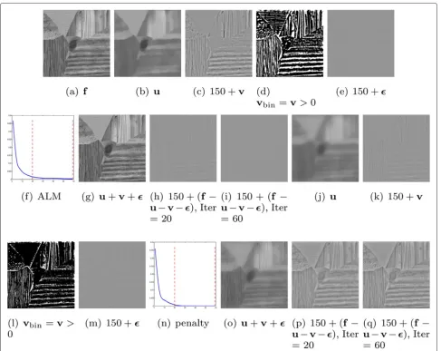
Fig. 7The comparison of ALM (a–i) and QPM (j–q) for the DG3PD model with the same parameters and 20 iterations:β4=0.025 ,θ=0.9 ,c1=10 , c2=1.3 ,cμ1=cμ2=0.03 ,γ=1 ,S=L=32 ,δ=5. We observe that the error image of QPM still contains geometry and texture information;
see after 20 iterations inpand after 60 inq. Using QPM for constrained minimization is similar to decomposing the original image into four parts, namely cartoon (j), texture (k), residual (m), and error (p). The amount of information in the error image by QPM strongly depends on the choice of parameters(β1,β2,β3,β4). However, for ALM, the updated Lagrange multipliers(λ1,λ2,λ3,λ4)compensate for the choice of(β1,β2,β3,β4). Thus, the error numerically tends to0as the number of iterations increases, see the error image after 20 iterations inhand after 60 iterations ini
frequency modulated (AM-FM) functions. They decom-pose a fingerprint image into four parts, and this idea can be applied to the texture imagevobtained by the DG3PD method:
v≈a+[b·cos(C+S)]
Each of the four components is again highly compress-ible and can be stored with only a few bytes (see Figure 5 in [17]). This is remarkable and we would like to offer another perspective on the AM-FM model. Storing a minutiae template can be viewed as a lossy form of
fingerprint compression. The minutiae of a fingerprint are locations where ridges (dark lines) end or bifur-cate, and a template stores the locations and direc-tions of these minutiae. Several algorithms have been proposed for reconstructing the orientation field (OF) from a minutia template [42]. The continuous phase
C can be derived from the unwrapped reconstructed OF and the spiral phase S directly constructed from the minutiae template. Choosing appropriate values for
Fig. 8The Barbara image (d) with additive Gaussian white noise (σ=20) is decomposed by the Aujol and Chambolle model (a–c) and the DG3PD model (e–h) withδ=16 and the other parameters are the same as in Fig. 2. Comparingaande, we observe that the cartoon image u obtained by the DG3PD model (e) has a smoother surface and sharper edges thana. Comparing the texture images v, we note thatfis smoother and sparser thanb. In order to highlight the sparseness of the DG3PD texture, all positive coefficients are visualized as white pixels inh. For visualization, we add 150 to the value of the residualing. The residual ingstill contains some texture, but mainly the Gaussian noise which is obviously shown in the QQ plot (i). There are some differences at the end of the tail iniprobably due to the remaining texture and the numerical simulation of Gaussian noise
Fig. 9DG3PD decomposition of a latent fingerprint for segmentation (a) withδ=60.b–eThe ROI is obtained from the binarized texture vbinand
Fig. 10Latent fingerprint images from NIST SD27. The boundary of the foreground estimated by the DG3PD method is drawn inyellow(a–d)
quantization (WSQ) [44] which has been a compres-sion standard for fingerprints used by the Federal Bureau of Investigation in the USA. See Fig. 11f–h for appli-cation example of WSQ to the texture of the Barbara image.
A third, very good compression possibility is dictionary learning [40] with optimization of the dictionary for the texture componentv. For fingerprint images, this problem has recently been studied by Shao et al. [45].
7.3.3 Residual image compression
For image compression using DG3PD, we propose the following steps in this order: First, image decomposi-tionf = u+ v+. Second, a tailor-made, lossy, high
compression of the cartoon component u and the tex-ture componentv. Third, decompressinguandvin order to compute the compression residual image s = f − ud − vd, where ud is the cartoon image and vd the texture image after decompression. Fourth, compression ofs.
In steps two and four, the term “compression” denotes the whole process including coefficient quantization and symbol encoding (see [46] for scalar quantization, Huff-man coding, LZ77, LZW, and Huff-many other standard techniques).
Let beeu = u −ud, the difference between the car-toon component before and after compression, i.e., the compression error, andev = v−vd, then we can rewrite
r = f − ud − vd = u + v + − ud − vd = + eu + ev. Hence, the residual images computed in step four contains the residual componentplus the compres-sion errors of the other two components. Now, lossless compression can be achieved by lossless compression of s. If the goal is lossy compression with a certain target quality or target compression rate, this can be achieved by adapting the lossy compression of saccordingly. See Fig. 11 for the effects of different compression rates on the decompressed cartoonud and the decompressed texturevd.
An additional advantage of decompression beginning with ud, followed by vd and finally sd is the fast gen-eration of a preview image which mimics the effects of interlacing. In a scenario with limited bandwidth for data transmission, e.g., sending an image to a mobile phone, the user can be shown a preview based on the compressed, transmitted, and decompressed u image. During the transmission of the compressed v and s, the user can decide whether to continue or abort the transmission.
8 Conclusions
The DG3PD model is a novel method for three-part image decomposition. We have shown that the DG3PD method achieves the goals defined in the introduction much better than other relevant image decomposition approaches. The DG3PD model lays the groundwork for applications such as image compression, denoising, and feature extraction for challenging tasks such as latent fin-gerprint processing. We follow in the footsteps of Aujol and Chambolle [3] who pioneered three-part decomposi-tion and DG3PD generalizes their approach. We believe that three-part decomposition is the way forward to address many important problems in image processing and computer vision. Buades et al. [18] asked in 2010: “Can images be decomposed into the sum of a geo-metric part and a textural part?” Our answer to that question is no if an image contains other parts than cartoon and texture, i.e., noise or small-scale objects. Consider, e.g., the noisy Barbara image in Fig. 8d. If the sum of the cartoon and texture images shall recon-struct the input image f, a two-part decomposition has to assign the noise parts either to the cartoon or to the texture component. In principle, not even the best two-part decomposition model can fully achieve both goals regarding the desired properties of the cartoon and texture component simultaneously. The solution is that noise and small-scale objects which do not belong to the cartoon or texture have to be allotted to a third component.
In our future work, we intend to optimize the DG3PD method for specific applications, especially image compression and latent fingerprint processing. Issues
for improvement include the data-driven, automatic parameter selection, and the convergence rate (can the same decomposition be achieved in fewer iterations?) Fur-thermore, we plan to explore and evaluate specialized compression approaches for cartoon, texture, and residual images.
Additionally, a very interesting application for the residual component can be biometric liveness detection. Recently, Gragnaniello et al. [47] have concluded that high-pass filtering before computing local image descrip-tors improves the accuracy of their proposed iris live-ness detection algorithm. The residual image obtained by DG3PD contains the high-frequency components of the input image. Applications of DG3PD to iris or fin-gerprint liveness detection [48, 49] are therefore very promising. A survey of local image descriptors for fin-gerprint, iris, and face liveness detection can be found in [50].
Optimal solutions of transportation problems are the key to compute the earth mover’s distance (EMD) or Wasserstein distance [51]. Recently, Brauer and Lorenz [52] discussed an interesting connection between Meyer’s G-norm and transportation problems. Solving trans-portation problems for images of dimension 512 ×512 pixels or larger can be a computationally extremely challenging problem (depending on the number of producers and consumers, and their distribution over the image domain) even for state-of-the-art methods such as the shortlist method [51]. However, in the special case of p = 1, the Kantorovich-Rubinstein duality provides a loophole which allows it to avoid solving the associated transportation problem. Based on this property, Brauer and Lorenz [52] proposed a three-part image decomposition with transport norms. Lellmann et al. [53] proposed the use of transport norms for image denosing and two-part image decomposi-tion. We believe that the commonalities between the Vese-Osher model [9], Meyer’s G-norm, and the recently proposed models using transport norms deserve further research.
Appendix
Fig. 12 a–fComparison of decomposition results by the ROF [1], VO [9], SED [11], TVG [12], and DG3PD models. Parameters for DG3PD are
Algorithm 1The Discrete DG3PD Model
Initialization: u(0)=f,v(0)=(0)=r(l0)L−1 l=0 =
w(s0) S−1
s=0 =
g(s0) S−1
s=0 =
λ(0) 1l
L−1 l=0 =
λ(0) 2a
S−1 a=0=λ
(0) 3 =λ(
0) 4 =0.
fort=1 ,. . .,Tdo 1. Compute
r(bt)L−1 b=0 ,
w(at) S−1
a=0 ,
g(at) S−1
a=0 ,v
(t),u(t),(t) ∈XL+2S+3:
r(bt) = Shrink 4
cos π
b
L u
(t−1)DT
n+sin
π b
L Dmu
(t−1)−λ(1t−1b )
β1 , 1
β1 5
, b=0 ,. . .,L−1
w(at) = Shrink 4
twa := g(at−1)−
λ(2t−1a )
β2 ,
μ1
β2 5
, a=0 ,. . .,S−1
g(at) = ReF−18A(t)(z)·B(t)(z),a=0 ,. . .,S−1
v(t)=Shrink 4
tv := β3
β3+β4 4S−1
s=0
cos,πs S
g(st)DTn+sin,πs S
Dmg(st)
−λ(3t−1)
β3 5
+ β4
β3+β4 4
f−u(t−1)−(t−1)+λ
(t−1) 4
β4 5
, μ2
β3+β4 5
u(t) = ReF−18X(t)(z)·Y(t)(z)
(t) = 4
f−u(t)−v(t)+λ
(t−1) 4
β4 5
− CST
4
f−u(t)−v(t)+λ
(t−1) 4
β4 ,δ
5
2. Updateλ(1tb)L−1 b=0 ,
λ(t)
2a S−1
a=0,λ
(t)
3 ,λ (t)
4 ∈XL+S+2:
λ(t) 1b = λ
(t−1) 1b + γβ1
r(bt)−cos
πb
L u
(t)DT
n−sin
πb
L Dmu
(t) , b=0 ,. . .,L−1
λ(t)
2a = λ(2t−1a ) + γβ2 ,
w(at)−ga(t), a=0 ,. . .,S−1
λ(t)
3 = λ (t−1) 3 + γβ3
4
v(t)− S−1
s=0
cos,πs S
g(st)DTn+sin,πs S
Dmg(st) 5
λ(t)
4 = λ(4t−1) + γβ4 ,
f−u(t)−v(t)−(t)
end for
A(z) =
β21mn+β3
sinπa S (z
−1
1 −1)+cos
πa S (z
−1
2 −1) sin
πa
S (z1−1)+cos
πa S (z2−1)
−1
,
B(z) = β2 .
Wa(z)+2a(z) β2
/
+ β3
sin,πa S
(z−11 −1)+cos,πa S
(z−12 −1)× ⎡
⎣V(z)− s=[0 ,S−1]\{a}
cos,πs
S
(z2−1)+sin
,πs S
(z1−1)
Gs(z)+3( z) β3
⎤ ⎦,
X(z)=
-β41mn+β1 L−1 l=0 . sin π l L (z
−1
1 −1)+cos
π l L (z
−1
2 −1)
/ . sin
π l
L (z1−1)+cos π
l
L (z2−1) /6−1
,
Y(z)=β4 .
F(z)−V(z)−E(z)+4(z) β4
/
+β1 L−1 l=0 . sin πl
L (z −1
1 −1)+cos
πl
L (z −1
2 −1)
/ .
Rl(z)+1l( z) β1
/ .
Choice of Parameters
μ1=cμ1β2·max
k∈++twa[k]++, μ2=cμ2(β3+β4)·maxk∈(|tv[k]|) andβ2=c2β3,β3=
θ

![Fig. 9 DG3PD decomposition of a latent fingerprint for segmentation (a) with δ = 60. b–e The ROI is obtained from the binarized texture vbin andmorphological postprocessing as described in [57]](https://thumb-us.123doks.com/thumbv2/123dok_us/908772.1588625/14.595.57.538.88.422/decomposition-fingerprint-segmentation-obtained-binarized-andmorphological-postprocessing-described.webp)

