R E S E A R C H
Open Access
Active stereo platform: online epipolar
geometry update
Abdulla Mohamed
1*, Phil Culverhouse
1, Angelo Cangelosi
1and Chenguang Yang
1,2Abstract
This paper presents a novel method to update a variable epipolar geometry platform directly from the motor encoder based on mapping the motor encoder angle to the image space angle, avoiding the use of feature detection algorithms. First, an offline calibration is performed to establish a relationship between the image space and the hardware space. Second, a transformation matrix is generated using the results from this mapping. The transformation matrix uses the updated epipolar geometry of the platform to rectify the images for further processing. The system has an overall error in the projection of ± 5 pixels, which drops to ± 1.24 pixels when the verge angle increases beyond 10°. The platform used in this project has 3° of freedom to control the verge angle and the size of the baseline.
Keywords:Active stereo vision, Epipolar geometry, Calibration, Binocular vision, Real-time update
1 Introduction
Stereo vision has been applied to many applications in different fields to make precise measurements and to ex-tend the working volume. In industrial applications, ste-reo vision has been used in control measurement and deflection detections [1–3]. In agriculture applications, stereo vision is used intensively in collecting data and the locations of fruits [4, 5]. This paper presents work done on an active stereo vision platform that is
inte-grated with a GummiArm robot [6] to identify the
pos-ition and quality of fruits. The platform is used to track an object and reconstruct the 3D shape of the object by updating the epipolar geometry.
The calibration process in a stereo vision system con-sists of calculating the parameters of the system both in-ternal and exin-ternal, such as the pixel size, focal length, and image size. External parameters define the orienta-tion and posiorienta-tion of the cameras in 3D space. In an or-thogonal stereo system or fixed system, the calibration is well defined using Zhang’s calibration algorithm [7]. The output of the calibration is used in the rectification process. Rectification is used to transform the left and right images to be parallel to the epipolar plane and
co-linear to the baseline [8]. This transformation
simplifies the next process, which is the correspondence, where the search across the scanning line becomes 1D instead of 2D.
Vergence cues are used by humans to focus visual atten-tion on a target, i.e., by keeping both eyes focused on the same object. Disparities generated using active stereo vi-sion depend on updates of the epipolar geometry. A feature-based algorithm can be used to compute the fun-damental matrix [9–12]. Such studies focus on matching the features between the left and right images every time there is a change in the system to compute the fundamen-tal matrix. A drawback to this method is the presence of failures when matching features. This leads to errors in the computation of the fundamental or homography matrix.
Another approach combines the image features and the motor angle to correct the errors in feature match-ing. Thacker and Mayhew (1991) used a Kalman filter on the encoder readings to predict the position of the object in the next frame [13].
Changes in the epipolar geometry occur because of changes in the camera angle and the position of the camera. These changes are measured by shaft encoders and are used in the control of camera positions. Dankers et al. developed an online calibration process for the
* Correspondence:[email protected]
1Centre for Robotics and Neural Systems, Plymouth University, Plymouth, UK Full list of author information is available at the end of the article
CeDAR head [14]. Their work was built on static system rectification [15], where the perspective projection matrix (PPM) found by the standard calibration process for the left and right cameras was used to locate the mapping be-tween the two images. The PPM was decomposed, and a new PPM and transformation between the left and right images were used to make the epipolar line parallel to the baseline. Dankers et al. modified the algorithm so that the rotating angle of the left and right images was replaced by the angle of the encoder of each camera [14]. Both the motor angle and the image were captured at the same time. However, even though this process was quite fast, it required a system with highly accurate manufacturing; it is very difficult to correctly place the rotating axis of the motor interacting with the camera origin, and this can lead to an error with the baseline.
Kwon et al. designed another approach to calibrate ac-tive stereo vision [16]. Their method treats the system as a kinematic chain that links the camera to its pan and tilt joints. By creating a kinematic chain between the joints and the camera and initializing the system, a cali-bration at the zero position of the system can be used to generate calibration matrices for the new positions. The motor angle transforms to the image coordinates via the transformation matrix between the image and the motor. Even though this method takes into account the position of the origin of the camera, if it is not intersected by the rotating axis, the error is accumulative during the run-ning time because of the integration of the differences computed between the old and new angles.
Hart et al. developed a calibration algorithm using a hu-manoid head and controlling the stereo verge angle [17]. The algorithm starts with an offline process where the es-sential matrix of each camera at two different orientations is computed, and then, the properties of the system are decomposed from the fundamental matrix. The centers of each camera and the rotation matrix are calculated using Rodrigues’ rotation formula [18]. These parameters are used at run time to compute a new epipolar geometry using the motor angle by inverting the process offline. An experiment was performed to evaluate the algorithm using the standard calibration process and to compare the result to the new algorithm. The result showed a mean difference between the two methods of 2.38 pixels. However, their al-gorithm used the difference between the encoder readings of each orientation and not the absolute angle. This led to an accumulation of errors with time.
Sapiens et al. investigated in real time the parameters of the stereo vision system during operation [19]. Their system maps the angle of the motor encoder to the image space by calibrating the system offline. The offline calibration finds a linear equation that maps the value of the motor angle to the image space angle. The algorithm in this study calculates the homograph of each image
(left and right) and decomposes the matrix to find the value of the angle in image space. This process was re-peated at a different motor angle, and the results were used to determine the relationship between the motor angle and the image area. In addition, they determined the properties of a common homograph with the same features at different angles. All of these processes were performed during an offline process. A linear equation was generated to make a map between the motor space and the image space using the motor angle as input. During operation, the homographs of both the left and right images were calculated using this equation and the motor angle. From the homographs, the fundamental matrix was calculated and used to rectify the images. This equation works linearly within the range of−20° to 20°, with an error of 1.03 pixels at 0° that increases to 3.28 pixels at 20°. These results were compared to the conventional calibration process. In this study, the model coefficient was fixed throughout the range of an-gles. This assumption requires a high-precision manu-facturing process to maintain the origin of the camera as close to the rotating angle as possible.
Both Kwon et al. [16] and Sapiens et al. [19] have per-formed similar studies of transforms from the motor angle to the image angle. Kwon et al. [16] worked with larger an-gles (from −45° to 45°) compared to Sapiens et al. [19],
whose work was limited to −20° to 20° for each camera.
However, Kwon et al. included the tilting angle, and their study better placed the origin of the camera [16]. Hart et al. used the angle of the motor encoder to estimate the es-sential matrix, which results in an error in the value of the matrix [17]; conversely, Sapiens et al. corrected the motor angle via pre-processing [19].
In our study, the active stereo vision platform requires an algorithm to update the epipolar geometry in real time with a measurement of the change made by the motors. We avoided the use of traditional methods that require finding features in both images and matching these features to compute the new epipolar geometry [12]. Such feature-based algorithms fail in most cases because of feature matching or environments that con-tain fewer features than the required amount to compute a new geometry. Moreover, the working range of the platform was increased to ± 60° compared to [16].
depth to allow an accurate rectification process for the
images generated by the system under different
arrangements.
The rest of the paper is organized as follows. The epipo-lar geometry and the process of computing the parameters in image space are presented in Section 2. Section3 pre-sents the process of collecting the data using a stereo cali-bration algorithm and the setup used to evaluate the algorithm. In Section4, the results and discussion are pre-sented, and finally, the paper concludes in Section 5.
2 Methods
This section introduces the algorithm used to produce the disparity map and depth measurement while the camera tracks an object without the need to constantly recalibrate the system. The process of updating the geometry online is described in this part. The method of updating the configuration of the system has two stages. The first stage is the offline calibration process using Zhang’s calibration algorithm [7], where the output of this algorithm is the PPM and distortion matrix for each camera, as well as the translation and rotation matrices between the left and right cameras. The PPM and distor-tion matrix contain the internal parameters for each camera, and these parameters are fixed at all times. The translation and rotation matrices contain the external parameters of the system and are constantly changing.
Figure 1 shows the outer parameters of the system.
The origin of the system is set, as is frequently done in computer vision, with the left origin as the origin of the system [20]. Therefore, the essential matrix describes the rotation and translation from the left image to the right image. In the offline calibration stage, the calibration was done under different geometric configurations. This process is used to find the relationship between the rota-tion angle in the image space and the platform space and to apply this to the translation.
The second stage of the calibration is online calibra-tion, where the generated relationship between the image space and the platform space is used to update
the essential matrix. The essential matrix is used in the rectification process.
2.1 Single-camera model
We start with a single-camera model that describes a pinhole camera system. This model is also used to de-scribe the CMOS sensor in the cameras used in this pro-ject. The center of the camera isO, which is the center
of the Euclidean coordinate system. The image plane π
coincides with the z-axis, and the distance between the origin and the image plane is the focal lengthf.
Suppose a pointWwith coordinates W= [X Y Z]Tset in the front image plane. A projection point w= [x y]T on the image plane will form when we draw a line from
Wto the origin of the cameraO. This creates a mapping from 3D space to 2D space. Using a homogeneous co-ordinate to map between points, we get Eq. (1):
w¼PW ð1Þ
where W= [X Y Z1]Tand w= [x y 1]Tare homogenous vectors andPis the camera projection matrix.
The camera projection matrix P contains the internal
and external parameters:
P¼AR R½ jt; ð2Þ
whereAis a 3 × 3 matrix describing the internal proper-ties of the camera (Eq. (3)), whereαxandαyare the focal lengths in pixels in the x and y directions, respectively, and sis a skew parameter, which, in most new cameras, is zero [18].Randtare external parameters that refer to the transformation between the camera and world co-ordinate, where R is a 3 × 3 rotation matrix of rank 3 andtis a translation vector.
A¼
αx s x0
0 αy y0
0 0 1
2 4
3
5: ð3Þ
The calibration process for a single camera depends on Eq. (1) to provide the point coordinates of wand W
that the image coordinate found by applying corner
detection and the points in the world coordinate given by measuring the distance between the corners in the checkerboard. By finding these points, the camera pro-jection matrix can be determined using algebra. A
well-known algorithm that can be used to find P is y
using the algorithm of Zhang (2000) [7].
2.2 Stereo model
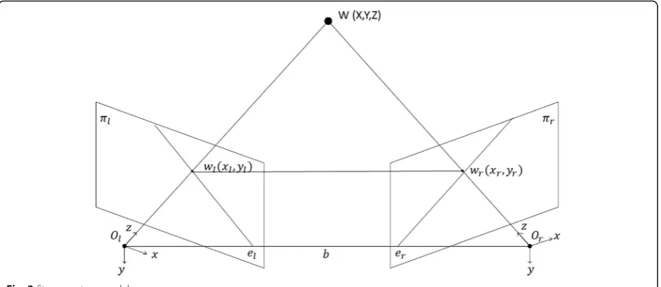
In the two-camera model, the same process as that for a single camera is applied. In this section, the parameters with subscript letters land rare used to refer to the left and right camera models, respectively. Figure2shows the model that is studied in this section. The distance between the two origin cameras isBand is referred to as the base-line. Supposing that both cameras look at the same point in the worldW= [X Y Z]T, a pointwwill be projected onto both image planeswl= [xlyl] andwr= [xryr].
From the model, a plane is formed when Ol, W,
andOr are connected. This plane is called the epipolar
plane. If we knowwl, we can findwrby searching along
a line lr=er×wr. This line is called the epipolar line.
From the epipolar line, lr=er×wr= [er] ×wr, where [er]
is the cross product, and because we know that wr is
mapping towl, we get the relationwr=H wl.His a 3 ×
3 homography matrix of rank 3 that describes the map-ping between two points. By combining both equations, we get lr= [er] ×H wl=F wl, where F= [er] ×H and is
called the fundamental matrix [21].
The fundamental matrix (F) can be extended to
in-clude the camera projection matrix, as shown Eq. (4),
where Pþl is the pseudoinverse of Pl. The fundamental
matrix defines the internal and external parameters of the stereo vision system. F is a 3 × 3 matrix of rank 2.
F¼½ er PrPþl: ð4Þ
For a stereo vision rig, the projection camera matrix satisfies Eqs. (5) and (6), whereRandtrepresent the ro-tation and translation between the left and right origins.
Olis the origin of the rig.
Pl¼½Ij0 ð5Þ
Pr¼½Rjt: ð6Þ
The fundamental matrix should satisfy Eq. (7), where
wllies on the epipolar linelr=Fwl[21]:
wrFwl¼0: ð7Þ
Equations (5) and (6) are in normalized coordinates, and solving them, we obtain Eq. (8):
E¼½ tR¼R RTt
: ð8Þ
The essential matrix (E) describes the transformation between the left and right origins in normalized image coordinates. TheEmatrix has similar properties to theF
matrix in its correspondence between w^l and w^r in
nor-malized coordinates [21]:
wbrEwbl¼0: ð9Þ
The essential matrix is used to compute the distance to the pointW(X,Y,Z) seen by both cameras. Using the essential matrix means that there will be 6° of freedom: 3° from the rotation angle and 3° from the translation. In our system, the rotation angle around they-axis and the translation along the baseline are not fixed. These two parameters were selected because they change the visual view of the camera.
The calibration process used in stereo vision is the same when a checkerboard is used as a reference to the points in the world coordinate and image processing is used to find the points in the image coordinate. The calibration process is first done on each camera separ-ately to find the projection camera matrix for each cam-era, and then, these matrices are used to calculate the essential matrix to find the external geometry parame-ters between the cameras.
2.3 Rectification algorithm
The disparity is the difference between the same points in the left and right images. The calibration process gen-erates the parameters used to rectify the images, where the rectification process is the transformation of the left and right images to obtain the same horizontal epipolar lines. The rectification process used in this study is based on Bouguet’s algorithm [20].
The process starts by dividing the rotation matrix R
that is responsible for rotating the right image into the left image into two rotating matrices,Rland Rr, for each
image. These two rotation matrices rotate the left and right images by a half rotation. This rotation aligns both image planes with the baseline, but the images are not aligned in the raw data. Therefore, we find a correction matrix to rotate the epipolar lines into infinity and align them horizontally with the baseline.
In the stereo model, it is assumed that the left camera was set as the origin of the system. Starting with the epi-pole point e1l in the left image and connecting to the epipole point e1r in the right image, the point is trans-lated along the baseline that defines the translation vec-torT. This leads to Eq. (10):
e1¼ T
T
k k: ð10Þ
Using the cross product ofe1will generatee2, which is
orthogonal to the focal length ray. This results ine2
be-ing orthogonal toe1. The result is shown in Eq. (11):
e2¼
−TyTx0
T
ffiffiffiffiffiffiffiffiffiffiffiffiffiffiffiffiffi
T2xþT2y
q : ð11Þ
The last vector ise3, which is orthogonal toe1and e2,
and can be calculated via a cross product:
e3¼e1e2: ð12Þ
Now, we add these vectors into the correction matrix
Rcorr, which transforms the epipolar lines to be infinite
and parallel with the baseline by rotating the image about the projection center.
Rcorr¼
eT1
eT
2
eT3
2 4
3
5: ð13Þ
Rcorris multiplied by the split rotation matrix to form
correction rotation matrices for the left and right images.
Rlcorr ¼RcorrRl ð14Þ
Rrcorr¼RcorrRr: ð15Þ
This leads to the importance of a given rotation matrix and translation matrix to rectify an image. The rotation and translation matrices are taken from the essential matrix, i.e., decomposing the essential matrix allows the rotation and translation matrices to be calculated.
2.4 Online geometry update
This subsection integrates the above discussion to gener-ate a relationship between the image angle and the motor encoder angle. Mapping between motor space to image space lead to errors if we use the encoder angle direct to the image angle [22].
As explained in the above section, the process is di-vided into two parts: an offline calibration process and an online geometry update. The offline calibration calcu-lates the essential matrix and the internal parameters of the cameras. The essential matrix is decomposed to gen-erate the rotation and translation matrices. The transla-tion matrix is a pure translatransla-tion from the left to right camera origins.
In theory, the rotation matrix should be equal to the pure rotation around they-axis. However, in reality, this assumption is not valid because of the actual installation of the camera on the platform and the installation of the camera sensor. The calibration result returns the rota-tion matrix, including these small values around the x -and z-axes. Therefore, the rotation matrix returns three angles. The complete rotation matrix is a product of multiplying the rotation matrices in XYZ order:
R¼Rxð Þ ψ Ryð Þ θ Rzð Þ∅ : ð16Þ
The rotation matrix is solved to return the individual angle. These angles are recorded as the image space
an-gles. The most important angle is θimg, which changes
the angle around they-axis.
The calibration process is done 30 times with different configurations (different verge angles) and each time the
encoder verge angle θencoder is recorded. The complete
θimg¼eþηθencoder; ð17Þ
where e refers to the error due to the mechanical
mis-alignment and lens distortion andηis an estimated fac-tor to correct the encoder angle.
2.5 Disparity
After the rectification of the system, the generated left and right images are used to compute the disparity map. Correspondence is then established, following the
extensive literature, for example [23]. The primary
junction of correspondence is to find the point in the right image to match the point in the left image and then calculate the differences in the x-axis. These dif-ferences are called the disparity.
The semi-global block-matching algorithm (SGM) [24]
is used in this study to evaluate the disparity map of the rectified images. SGM is a global stereo matching algo-rithm using multiple direction searches (pixel-wise) to smoothen the output, where the matching cost used in SGM is mutual information to overcome issues in light-ing, different time exposures, and reflection [25]. The pixel-wise method calculates the final disparity by sum-ming the total cost of the disparities at different angles from the scan line. This approach ensures that there is some smoothness in the disparity.
E Dð Þ ¼X
P
C p;Dp
þX
qϵNp
P1T D p−Dq¼1
þX
qϵNp
P2T D p−Dq>1
0 @
1 A:
ð18Þ
Equation (18) represents the minimized cost function
used by SGM, wherepand qare the pixel indices in the
image, C(p,Dp) is the cost of disparity matching based
on the intensity,Nprepresents the neighbor of the pixel
p, and P1and P2are constraints to penalize the change
in the disparity, whereP1represents the change equal to
1 andP2represents the change greater than 1 [26].
The disparity map is used to transform the pixel from the image coordinate in 2D into a world coordinate in 3D [X Y Z]T relative to the camera origin. This process is done using a triangulation approach in Eqs. (19)–(21). In Eq. (20), x and y represent the modified coordinates of the object in the image frame, b is the baseline,d is the disparity, andfrepresents the focal length.
Z¼ f b
d ð19Þ
Y¼ f y
Z: ð21Þ
2.6 Experiment
The platform used in this work is explained in details
in our previous work [27]. The setup of the
experi-mental system was divided into two configurations. The first configuration collected the data for the calibration process to find the actual parameters of the platform. The second configuration evaluated the new calibration algorithm.
2.6.1 Collecting data
This section explains the process of obtaining the data to help extract the parameters of the active stereo vision system. Exploring the parameters of the system and comparing the image space to the motor space required generating data for different platform setups, which meant setting different verge angles and baselines; 30 configurations of varying verge angles and five configu-rations for the baseline were selected.
In each configuration, a calibration process was
per-formed as explained in Section 2.2 to find the
parame-ters of the system using a calibration board. The board consists of an 8 × 6 array of black and white squares with sizes of 34.5 mm in height and width. The algorithm used to find the corners on the checkerboard also de-tected the 48 internal corners on the board. For a robust calibration, 15 images were taken of the calibration board at various positions and orientations as recom-mended by (Bradski and Kaehler, 2008).
To accelerate and improve the collection of data, the calibration process was automated using a Baxter robot, as explained in [27]. Automating the calibration process re-duced the time required to complete the calibration process by three times and improved the calibration result.
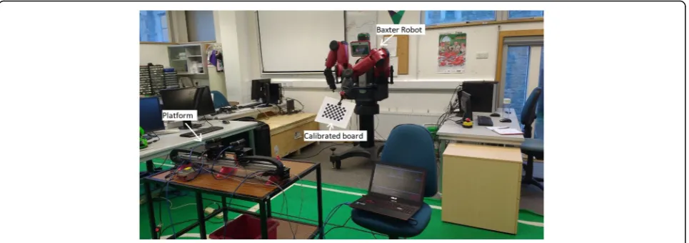
Figure 3 shows the data collection setup, where the
platform was installed in front of Baxter at a distance of 2 m, and the calibration board was fixed on the arm of the robot. A total of 40 positions and orientations of the board were pre-recorded using the Baxter teaching methods. A desktop PC was used to control Baxter, and a laptop was used to control the platform and perform the calibration process. A UDP connection was used to communicate between the PC and the laptop.
Figure4 shows a flowchart of the calibration process, where the process starts by setting the verge angle. The second step is to find the corner and to move the arm to a new position. This step was repeated until 15 sets of images were taken successfully with the corners de-tected. Then, the calibration process is started at the same time as the evaluation of the quality of the calibra-tion, when the output meets the requirement that the X¼ f x
projection error is less than 0.1, the calibration process is a success, and the system moves to a new configuration. If the projection error is larger than 0.1, the process repeats until it meets the requirement. This algorithm was re-peated 20 times to generate data for the analysis. The same process was used to calibrate the baseline.
2.6.2 Rectification
The calibration algorithm results in a rectified image where the epipolar lines of the left and right images be-come co-linear and parallel with the horizontal axis. To measure the performance of this rectification, a
projec-tion error measurement was used as described in [21].
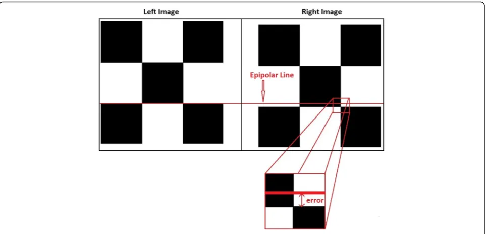
The projection error is defined as the difference between the pointy-axis in the left image and the point y-axis in the right image, as shown in Fig.5[28].
A calibration board was placed in different locations and orientations at distances between 1.5 and 2.5 m from the platform. This allowed us to obtain more data and to evaluate the calibration algorithm more accurately. As ex-plained in Section2.4, the geometry of the system needs to be updated when the configuration of the platform changes, and rectified images should then be generated. The rectified images are the output of the calibration algo-rithm, and these two images are used to evaluate the qual-ity of the calibration. The evaluation algorithm uses the calibration board to detect the corners of the left and right images and then calculate the root mean square error (RMS), i.e., Eq. (22). The output value is in units of pixels.
error¼
ffiffiffiffiffiffiffiffiffiffiffiffiffiffiffiffiffiffiffi
yli−yr i
2
q
ð22Þ
2.6.3 Surface compression
The data generated from the disparity map are used to create a 3D point cloud related to the system origin, which is a physical dimension of the scene. These data Fig. 3Baxter holding the checkerboard while the rig works on the calibration (in the lower left of the figure)
are used to evaluate the quality of the system in generat-ing the point cloud. A spherical object was placed in front of the system, and a 3D point cloud was generated for this sphere. These data were then compared to the ground truth of the sphere that was generated using a 3D model.
The iterative closest point (ICP) algorithm was used to translate and rotate the source of the point cloud to the reference by minimizing the differences [29]; that is, ICP was used to align the two point clouds. There are four steps that ICP uses in the alignment process, as described in the work of Rusinkiewicz and Levoy (2001) [30].
1. Apply the correspondent to the points where the strategy starts by selecting a point with a uniform distribution.
2. Use singular value decomposition to compute the rotation and translation between the reference and source point clouds.
3. Apply rotation and translation to the registered point cloud.
4. Calculate the error between the corresponding points by applying SSD.
The above steps were repeated until the error reached the threshold value.
To evaluate the generated sample (S) point cloud of
the platform, it was compared to the reference point cloud that was generated using a model, which we refer to as the ground truth (G). The Euclidean distance algo-rithm, Eq. (23), is used to compute the distance between each point in the source that lies near the point in the Fig. 5Definition of the error generated in the rectified images
reference point cloud. The differences between the sam-ple and the ground truth were calculated using the RMS using the Euclidean distance:
RMSerror¼
ffiffiffiffiffiffiffiffiffiffiffiffiffiffiffiffiffiffiffiffiffiffiffiffiffiffiffiffiffiffiffiffiffiffiffiffiffiffiffiffiffiffiffiffiffiffiffiffiffiffiffiffiffiffiffiffiffiffiffiffiffiffiffiffiffiffiffi
Sx−Gx
ð Þ2þ
Sy−Gy
2
þðSz−GzÞ2
q
:
ð23Þ
In the experiment, three spheres were used, with dif-ferent diameters (80, 125, and 150 mm). CAD software was used to generate the ground truth, which was then converted to a point cloud. These point clouds were set to have a subsampling between points equal to 1 mm in all directions (Fig.6a).
The generated point cloud from the platform is shown
in Fig. 6b prior to post-processing to remove the
sur-rounding points that do not belong to the sphere; the post-processing was done using the Point Cloud Library [31]. The setup of the experiment is shown in Fig.7.
The data were collected at different configurations
(verge angles from −6° to 12° and baselines from 55 to
250 mm) while the ball was placed at different positions between 1 and 2.5 m from the platform. A set of 10 samples was taken at each configuration.
3 Results and discussion
3.1 Offline calibration
The results of the offline calibration allow us to under-stand the geometry of the platform in depth; these data show the tolerance of the manufacturer and the repeat-ability of the motors. As explained in Section 2.4, the only variable axes are the verge angle (yaw) and the baseline (along with the y-axis), whereas the other axes are fixed, i.e., the pitch and roll angles and translation along they- andz-axes. These should be fixed in the dif-ferent configurations. The values of the roll and pitch angles are shown in Fig.8, where the roll angle is 0.526°, with a margin of error of ± 0.047°, and the pitch angle is
−0.433°, with a margin of error of ± 0.015°. These two
values were generated as a result of the assemble mis-alignment in the platform and cameras; as a technical note, Flea3 Point Gray cameras (FL3-U3-120S3C-C) have an accuracy of ± 0.5° of the sensor assembly. The same points apply to the result of the translation along the y- and z-axes (Fig.9). As shown in Fig.9, thez-axis reading is 3.6 mm, with a large margin of error of ± 2.3 mm, and this was the result of identifying the optical
Fig. 7The setup for the shape reconstruction using a sphere with a diameter of 120 mm
Fig. 8The result of the offline calibration process for the roll and pitch angles
center of the cameras. This leads to an issue with meas-uring the distance if it is assumed to be fixed. To resolve
the error in z-axis, a relationship was computed from
the calibration data to update the z-axis during the
changing of the configuration.
Theoretically, the verge angle is directly correlated to the motor angle. After processing the data in the offline calibration, the raw data related to the verge angle were generated and plotted against the sum of the encoder angles (Fig. 10). As shown in Fig. 10, the image angle generated by the offline calibration and the encoder angles show a linear relationship with a coefficient of determination equal to 99.93%. From
the data, η is equal to 0.9641, and the error value e
is equal to 0.5786. Inserting these values into Eq. (17) results in Eq. (24):
θimg¼0:5786þ0:9641θencoder: ð24Þ
Accordingly, Eq. (24) was used to update the image
angle by providing the encoder angle reading from the motor. This improved the updates of the geometry of the system. Comparing this result to that of Dankers et al., the epipolar geometry was updated in a more accurate process, which studied the platform in more detail before starting the online update [14]. This result will help im-prove the vision in humanoids, manipulator arms, and Fig. 10The image angle versus the motor angle. The image angle was calculated using the stereo calibration process, and the motor angle was measured using the encoders
mobile robots that use active stereo vision and will extend the working volume of the binocular vision.
3.2 Online geometry update
Equation (24) was used to calculate the image angle
based on the input of the encoder angle; the new image angle was then used to rectify the images. This process was done during the online running time, as described in Section 2.4. To evaluate the new algorithm, the pro-jection error was used as described in the experimental
section. The result of the projection error is shown in Fig.11. This result was collected at different verge angles and baselines, and the experiment was repeated 20 times. In general, the result shows that the platform and the online calibration algorithm have repeatability with a marginal range of ± 0.5 pixels, which gives us confidence in the ability of the platform for repeating tasks.
Figure11indicates that the projection error has a linear relationship with the verge angle when the baseline has a small value, e.g., a baseline of 50 or 100 mm. However, the
projection error increases with increasing baseline size. This could be a result of the misalignment in the roll angle, which was set in the opposite direction, or they dis-placement misalignment during the manufactures, which increases with the baseline. Moreover, the projection error increases by increasing the diverge angle, and drops when the platform starts to verge, the error is not constant; this is due to the position of the target: the images started to overlap, which led to a drop in the error. Figure11shows that, when the verge angle starts to increase, the projection error starts to decrease, where the target gets close to the horopter. At an angle of 6°, the projection error drops be-cause of the position of the target, which leads to zero dis-parity. The zero disparity reduces the disparity range and the error in the depth measurement.
A list of rectified images captured at different verge
angles is shown in Fig. 12. The colored lines show the
epipolar lines where the pixel in the left image is lying
on the same line. Figure12awas captured at the
paral-lel focal axis, and the rest were taken in 2° increments. This shows that the image sizes decrease with increas-ing verge angle; the red square represents the image size after rectification.
Figure13shows the disparity map of the rectified im-ages at different verge angles. The disparity shows the box that was used to evaluate the process. The corre-sponding process was based on the SGM algorithm with a window size of 5 × 5 pixels and a disparity number of 256. The size of the windows was selected based on the output of the projection error analysis (Fig.11) to cover
the potential error in the rectified image. At the same time, windows at this size will sharpen features, as dis-cussed in [18]. As shown in Fig. 13, the disparity map becomes more intense with increasing verge angle, where Fig.13fwith an angle of 10° is due to the overlap of the images. Because the disparity map can only pro-vide a visual analysis, the next section generates a point cloud to compare to the ground truth.
3.3 Surface compression
To demonstrate the quality of the disparity map, the dispar-ity was converted into a point cloud using the triangulation equations, as described in Section2.6.3. The ground truth point cloud was generated using a CAD model. A sample of the data used in the comparison is shown in Fig.14.
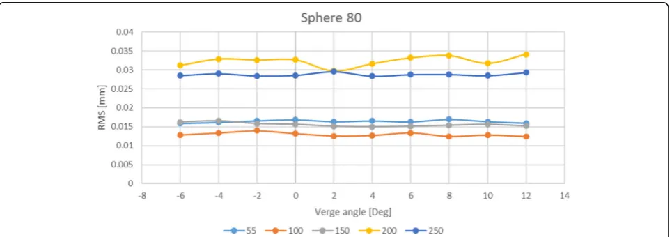
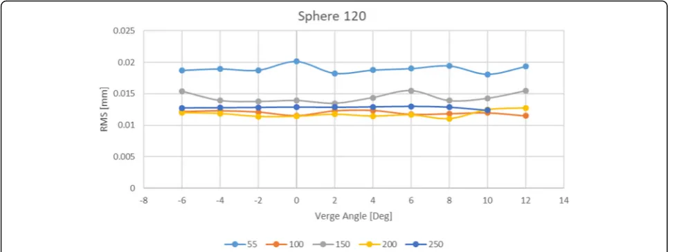
Figures 15, 16, and 17 show the result of computing
the RMS between the ground truth and the sample for three sizes of the sphere (80, 120, and 150 mm). The re-sult describes the sum of the differences of the points from the ground truth. Five different baselines (55, 100, 150, 200, and 250 mm) were used to generate samples at different verge angles (from−6° to 12°) with steps of 2°. The overall result has the same shape as the result of the projection error (Fig. 11) and shows that the result of the baseline with 100 mm has the lowest RMS and that an increase in the baseline led to an increase in the RMS. The RMS of the baseline with 55 mm has the highest RMS in the three cases because of the propor-tional error in measuring the depth in relation to the baseline, as described in [32].
However, the RMS of the verge angle shows a linear result at different verge angles, with a slight drop in the result at larger verge angles; this is because the overall error in the projection was four pixels, and five pixels were used to compute the disparity windows to over-come mismatching at the scan line. This result may lead to a misunderstanding in the use of the variable verge angle in computing the disparity if the result shows an approximate equal RMS at different verge angles. How-ever, to generate the sample, post-processing was per-formed on the sample to reduce the amount of RMS
points computed, and as shown in Section 3.2, the
dis-parity became smaller when the verge angle increases.
Moreover, the measurement of the depth approached the origin of the system, where the parallel focal length of the minimum depth was 1 m, and for the verge angle, the depth converged to 0.5 m. However, the size of the sphere does not affect the result of the object recon-struction; all results had an average RMS of approxi-mately 0.02 mm and a margin of error of ± 0.0039 mm at a confidence of 95%.
The drawback of this algorithm is that the size of the rectified image generated becomes smaller when the verge angle increases. This occurs due to the behavior of epipo-lar lines at verge angle (Fig.18). Moreover, the rectifica-tion process makes this line parallel with the baseline; therefore, the new image becomes smaller.
4 Conclusions
An active stereo vision platform with 3° of freedom, pro-viding individual camera pans with a shared variable baseline, was constructed and assessed for its depth resolution and repeatability. A study was performed using both traditional stereo disparity estimations and the camera verge angle to provide depth information.
The problem of computing the epipolar geometry of an active stereo vision system was studied to avoid trad-itional methods that use feature-based algorithms [12]. A relationship was found between the image angle and the encoder angle to update the epipolar geometry of the system directly from the encoder reading.
An offline calibration process was performed to find measurements in the image space of the platform, and then, these measurements were used to find the relation-ship between the image space and the encoder angle. A linear correlation was found between the image space and encoder angle with a shift of 0.5° in image space.
Fig. 15RMS error for a sphere with a diameter of 80 mm at different baselines and verge angles
The overall measurement of the epipolar geometry in image space was found using the offline calibration.
In order to evaluate the performance of the rectifi-cation algorithm, the projection error based on SSD
[21] was used. The maximum projection error that
the platform generates at de-verge is ± 5 pixels and when the platform starts to verge the error drop to ± 1.24 pixels at 12°. This compares to ± 2.38 pixels in the work of Hart et al [17]. This result shows that in-creases in the baseline increase the projection error, and increases in the verge angle decrease the projec-tion error and the effect of overlapping between the two images. A drawback of this algorithm is that the size of the new rectified images becomes smaller when the verge angle increases. The maximum verge angle that allowed the image to work with is 20°.
The disparity map depends on the quality of the rectification algorithm which the better the rectifica-tion the better the disparity map; therefore, experi-ments to evaluate the disparity map were conducted. The disparity maps show clear results in different configurations. Point cloud compressions were made with ground truth datasets to evaluate the quality of the shapes. These compressions show that the qual-ity of the shape has an average standard deviation of 0.0142 m and a margin of ± 0.0039 m.
Overall, the system improves the quality of the dispar-ity map by controlling the baseline and the verge angle. One of the main advantages of the system is the capabil-ity to focus on one target with reconstructing the 3D shape using a small disparity search area. As a result, the system extends the working volume space of robots.
Fig. 17RMS error for a sphere with a diameter of 150 mm at different baselines and verge angles
Future studies will automate the optimal baseline and verge angle based on the object position to reduce the error. In addition, the platform will be integrated with the GummiArm robot to harvest a tomato.
Abbreviations
CCD:Charge-coupled devices; CMOS: Complementary metal oxide semi-conductor; ICP: Iterative closest point; PCL: Point Cloud Library; PPM: Perspective projection matrix; RMS: Root mean squared; SGM: Semi-global matching; SSD: Sum of squared differences
Acknowledgements
This work is supported by the GummiArm robot.
Availability of data and materials
The data are available athttps://github.com/ahmohamed1/ activeStereoVisionPlatform.git.
Authors’contributions
The rest of authors are all my supervisors in the Centre for Robotics and Neural Systems, University of Plymouth and Zienkiewicz Centre for Computational Engineering, Swansea University. The work id is a part of a PhD program. AM wrote the paper, PC supervise the work and revised the paper at all stages and AC and CY revised the paper.
Ethics approval and consent to participate
Not applicable.
Competing interests
The authors declare that they have no competing interests.
Publisher’s Note
Springer Nature remains neutral with regard to jurisdictional claims in published maps and institutional affiliations.
Author details
1Centre for Robotics and Neural Systems, Plymouth University, Plymouth, UK. 2Zienkiewicz Centre for Computational Engineering, Swansea University, Swansea, UK.
Received: 16 February 2018 Accepted: 20 June 2018
References
1. PF Luo, YJ Chao, MA Sutton, Application of stereo vision to three-dimensional deformation analyses in fracture experiments. Optical Engineering. International Society for Optics and Photonics33, 81 (1994).
https://doi.org/10.1117/12.160877.
2. JJ Aguilar, F Torres, MA Lope, Stereo vision for 3D measurement: accuracy analysis, calibration and industrial applications. Measurement18, 193–200 (1996).https://doi.org/10.1016/S0263-2241(96)00065-6Elsevier
3. Li P, Chong W, Ma Y. Development of 3D online contact measurement system for intelligent manufacturing based on stereo vision. ed. by Osten W, Asundi
AK, Zhao H. AOPC 2017: 3D Measurement Technology for Intelligent Manufacturing. SPIE, pp. 66, 2017, doi:https://doi.org/10.1117/12.2285542
4. E Ivorra, AJ Sánchez, JG Camarasa, MP Diago, J Tardaguila, Assessment of grape cluster yield components based on 3D descriptors using stereo vision. Food. Control50, 73–282 (2015).https://doi.org/10.1016/J. FOODCONT.2014.09.004Elsevier
5. C Wang, X Zou, Y Tang, L Luo, W Feng, Localisation of litchi in an unstructured environment using binocular stereo vision. Biosystems Engineering145, 39–51 (2016).https://doi.org/10.1016/J.BIOSYSTEMSENG. 2016.02.004Academic Press
6. MF Stoelen, F Bonsignorio, A Cangelosi, inFrom Animals to Animats 14, ed. by E Tuci et al.. Co-exploring actuator antagonism and bio-inspired control in a printable robot arm (Springer International Publishing, Cham, 2016), pp. 244–255
7. Zhang Z, (2000) A flexible new technique for camera calibration. IEEE Transactions on Pattern Analysis and Machine Intelligence. IEEE, 22, 1330– 1334. doi:https://doi.org/10.1109/34.888718.
8. E Trucco, A Verri. (1998) Introductory techniques for 3-D computer vision. (Upper Saddle River, NJ, USA: Prentice Hall PTR).https://dl.acm.org/citation. cfm?id=551277.
9. Krotkov E, Henriksen K, Kories R, Stereo ranging with verging cameras. IEEE Transactions on Pattern Analysis and Machine Intelligence IEEE, 12, 1200– 1205 (1990). doi:https://doi.org/10.1109/34.62610.
10. S De Ma, A self-calibration technique for active vision systems. IEEE Trans. Robot. Autom.12, 114–120 (1996).https://doi.org/10.1109/70.481755
11. QT Luong, OD Faugeras, Self-calibration of a moving camera from point correspondences and fundamental matrices. Int J Comput Vis22, 261–289 (1997).https://doi.org/10.1023/A:1007982716991Kluwer Academic Publishers 12. M Bjorkman, JO Eklundh, Real-time epipolar geometry estimation of
binocular stereo heads. IEEE Trans. Pattern Anal. Mach. Intell.24, 425–432 (2002).https://doi.org/10.1109/34.990147
13. NA Thacker, JE Mayhew, Optimal combination of stereo camera calibration from arbitrary stereo images. Image Vis. Comput.9, 27–32 (1991).https:// doi.org/10.1016/0262-8856(91)90045-Q
14. Dankers A, Barnes N, Zelinsky A Active Vision—Rectification and Depth Mapping. Australian Conference on Robotics and Automation (2004). 15. A Fusiello, E Trucco, A Verri, A compact algorithm for rectification of stereo pairs.
Mach. Vis. Appl.12(1), 16–22 (2000).https://doi.org/10.1007/s001380050003
16. Kwon H, Park J, Kak AC, A new approach for active stereo camera calibration. in Proceedings 2007 IEEE International Conference on Robotics and Automation. IEEE, 3180–3185, (2007), doi:https://doi.org/10.1109/ROBOT.2007.363963. 17. J Hart, B Scassellati, SW Zucker, inCognitive Vision, ed. by B Caputo, M Vincze.
Epipolar Geometry for Humanoid Robotic Heads (Springer Berlin Heidelberg, Berlin, 2008), pp. 24–36.https://doi.org/10.1007/978-3-540-92781-5_3
18. Szeliski R, Computer vision: algorithms and applications (1st ed.). (Springer-Verlag, Berlin, 2010).https://dl.acm.org/citation.cfm?id=1941882. 19. Sapienza, M., Hansard, M. and Horaud, R. (2013), Real-time visuomotor
update of an active binocular head, Autonomous Robots. Springer US, 34(1–2), pp. 35–45. doi:https://doi.org/10.1007/s10514-012-9311-2. 20. Bradski GR, Kaehler A, (2008), Learning OpenCV: computer vision with the
OpenCV library. O’Reilly
21. R Hartley and A Zisserman, Multiple View Geometry in Computer Vision (2 ed.). (Cambridge University Press, New York 2003).https://dl.acm.org/ citation.cfm?id=861369.
22. Kyriakoulis N, Gasteratos A, Mouroutsos SG (2008), Fuzzy vergence control for an active binocular vision system. in IEEE (ed.) 7th IEEE International
Conference on Cybernetic Intelligent Systems, CIS 2008, 1–5 (2008). doi:
https://doi.org/10.1109/UKRICIS.2008.4798931.
23. D Scharstein, R Szeliski, A taxonomy and evaluation of dense two-frame stereo correspondence algorithms. Int. J. Comput. Vis.47, 7–42 (2001).
https://doi.org/10.1023/A:1014573219977.
24. H Hirschmuller, Accurate and efficient stereo processing by semi-global matching and mutual information. In Proc. IEEE Int. Conf. Computer Vision Pattern Recognition (CVPR)2, 807–814 (2005)
25. Banz C, Hesselbarth S, Flatt H, Blume H, Pirsch P (2010), Real-time stereo vision system using semi-global matching disparity estimation: architecture and FPGA-implementation. in 2010 International Conference on Embedded Computer Systems: Architectures, Modeling and Simulation. IEEE, 93–101. doi:https://doi.org/10.1109/ICSAMOS.2010.5642077.
26. H Hirschmuller, Stereo processing by semiglobal matching and mutual information. IEEE Trans. Pattern Anal. Mach. Intell.30, 328–341 (2008).
https://doi.org/10.1109/TPAMI.2007.1166
27. A Mohamed, PF Culverhouse, R De Azambuja, A Cangelosi, C Yang, Automating active stereo vision calibration process with cobots. IFAC-PapersOnLine50, 163–168 (2017).https://doi.org/10.1016/J.IFACOL.2017.12.030Elsevier 28. David A. Forsyth, Jean Ponce, Computer vision: a modern approach,
Prentice Hall Professional Technical Reference, 2002.
29. PJ Besl, ND McKay, A method for registration of 3-D shapes. IEEE Trans. Pattern Anal. Mach. Intell.14(2), 239–256 (1992)
30. S. Rusinkiewicz and M. Levoy, Efficient variants of the ICP algorithm, in Proceedings Third International Conference on 3-D Digital Imaging and Modeling (2001), pp. 145–152.
31. Rusu, R. B. and Cousins, S., 3D is here: Point Cloud Library (PCL), in 2011 IEEE International Conference on Robotics and Automation. IEEE (2011), pp. 1–4. doi:https://doi.org/10.1109/ICRA.2011.5980567.
32. T Dang, C Hoffman, C Stiller, Continuous stereo self-calibration by camera parameter tracking. IEEE Transactions on Image Processing